On Measuring Process Model Similarity based on High-level Change Operations
Chen Li1, Manfred Reichert1, and Andreas Wombacher2
1 Information System group, University of Twente P.O.Box 217, 7500 AE Enschede, The Netherlands
{lic,m.u.reichert}@cs.utwente.nl
2 Database group, University of Twente P.O.Box 217, 7500 AE Enschede, The Netherlands
a.wombacher@utwente.nl
Abstract. For various applications there is the need to compare the similarity between two process models. For example, given the as-is and to-be models of a particular business process, we would like to know how much they differ from each other and how we can efficiently transform the as-is to the to-be model; or given a running process instance and its original process schema, we might be interested in the deviations between them (e.g. due to ad-hoc changes at instance level). Respective considerations can be useful, for example, to minimize the efforts for propagating the schema changes to other process instances as well. All these scenarios require a method to measure the similarity or distance between two process models based on the efforts for transformation. In this paper, we provide an approach using digital logic to evaluate the distance and similarity between two process models based on high-level change operations (e.g. to add, delete or move activities). In this way, we can not only guarantee that the transformation results in a sound process model, but also ensure that the efforts are minimized.
1 Introduction
Business world is getting increasingly dynamic, requiring from companies to con- tinuously adapt theirProcess-Aware Information Systems (PAIS) [6] in order to cope with the frequent and unprecedented changes in their business environ- ment [23, 25]. Organizations and enterprises need to continuously Re-engineer their Business Processes (BPR), i.e. they need to be able to flexibly upgrade and optimize their business processes in order to stay competitive in their mar- ket. Furthermore, PAIS should allow for process flexibility, i.e., they should allow users to deviate from the standard process model at the instance level if required.
Finally, organizational learning should be supported by analyzing these process instance deviations. The latter provides useful information about the past which can be utilized by a company to evolve and optimize its business processes and supporting PAIS [17].
The pivotal research on process flexibility over the last years [3–5] has pro- vided the foundation for dynamic process change to reduce the cost of change
II
in PAIS. In this context, business process flexibility denotes the capability to reflect externally triggered change by modifying only those aspects of a process that need to be changed, while keeping the other parts stable, i.e., the ability to change or evolve the process without completely replacing it [4]. When com- paring two process models, we would like to be able to calculate their minimal difference based on high level changes so that if we need to transform one model to another, efforts can be reduced and the transformation can go smoothly (i.e.
we do not need to re-implement the new process model from scratch, but only apply these high level changes either at process type or process instance level).
Several approaches like ADEPT [5], WASA [10] or TRAM [9], have emerged to enable full lifecycle support in PAIS (for an overview see [7]). All these systems support ad-hoc deviations at the instance level and record them inchange logs.
Thus, they provide additional information when compared to traditional PAISs which only recordexecution logs.
1.1 Problem Statement
Based on the two assumptions that: (1) process models are block-structured and (2) all activities in a process model have unique labels, this paper deals with the following research question:
Given two process modelsS andS0, how much do they differ from each other in terms of high-level change operations? And what is the minimal effort, i.e.
the minimal number of change operations needed to transform S intoS0? Clearly, our focus is on minimizing the number of changes necessary to trans- form process modelSinto process modelS0. However, soundness of the resulting process model should be also not sacrificed. When modifying a process model, we apply the high-level change operations as introduced by the ADEPT method [5]
to guarantee soundness. By considering high-level change operations, we can dis- tinguish ourselves from traditional similarity measures like graph isomorphism [2] or sub-graph isomorphism [24], which only consider basic change primitives like the insertion or deletion of single nodes and edges. At process type level, answering this question will lead to better cost efficiency when performing BPR, since the efforts to implement the corresponding changes in the supporting PAIS is minimized. At process instance level, answering this question can reduce the efforts to propagate the process type changes to the running instances [7, 18];
or when there are thousands of instances, the derived differences between the original process model and each process instance can be used as a set of pure and concise logs for process mining [17].
1.2 Contribution
Previous work on ADEPT [5] has provided the technical foundation for users to flexibly change process models at both the process type and the process instance level. For example, users may dynamicallyinsert, delete ormovean activity [5]
at these two levels. In addition, snapshot differential algorithms [1], known from database technology, can be used as a fast and secure method to detect the
III change primitives (e.g. concerning differences of the activities or control flow edges) needed to transform one process model into another.
Based on the ADEPT framework and snapshot differential algorithm, this paper applies Digital Logic in Boolean Algebra [20] to provide a new method to transform a process model to another based on high-level change operations. This method does not only minimize the number of changes needed in this context, but also guarantees soundness of the changed process model, i.e. the process model remains correct when applying a high-level change operation. Our paper also provides the two measures ofprocess distance andprocess similarity based on high-level change operations. Such measures can be used to determine how difficult it is to transform a process model into another, and how different two process models are.
The remainder of this paper is organized as follows: Section 2 introduces backgrounds needed for the understanding of this paper. In Section 3, we dis- cuss reasons and difficulties for deriving high-level change operations. Section 4 describes an approach to detect the changes between two block-structured pro- cess models, and Section 5 discuss related work. The paper concludes with a summary and outlook in Section 6.
2 Backgrounds
A process model S = (N, E, . . .) ∈ P is defined as a Well-Structured Marking (WSM) Net [5].P stands for all the possible process models.N constitutes a set of activities ai associated to S and E is a set of control edges linking all these activities. To limit the scope, we assume process models to be block structured.
A detailed description and correctness issues of WSM Nets are out of the scope of this paper, (see [22]).
We assume that a process change is accomplished by applying a sequence of change operations to a given process model S over time [5]. Such change operations modify the initial process model by altering the set of activities and/or by changing their order relations. Thus, each application of a change operation to a process model results in another process model. In this context, we define high-level change operations on a process model as follows:
Definition 1 (Change in Process Model).Let P be the set of possible pro- cess models andCthe set of possible process changes. LetS, S0∈ P be two process models, let ∆ ∈ C be a process change, and let σ =h∆1, ∆2, . . . ∆ni ∈ C∗ be a sequence of process changes performed on initial process model S. Then we can define:
– S[∆iS0 iff∆ is applicable to S andS0 is the process schema resulting from the application of∆ toS.
– S[σiS0 iff ∃ S1, S2, . . . Sn+1 ∈ P with S = S1, S0 = Sn+1, and Si[∆iSi+1
withi={1, . . . n}.
Examples of high-level change operations and their effects on a process model are depicted in Table 1. Issues concerning the correct use of these operations and
IV
Table 1.Examples of High-Level Change Operations on Process Schemas
Change Operation opType subject paramList
∆Applied to S
insert(S, X,A,B, [sc]) insert X S,A,B, [sc]
Effects on S:inserts activity X between activity setsAandB.
It is a conditional insert if [sc] is specified (i.e. [sc] =XOR)
delete(S, X, [sc]) delete X S, [sc]
Effects on S:deletes activity X from S, i.e. X turns into a silent activity. [sc] is specified ([sc] =XOR) when we block the branch with X, i.e. the branch which contains X will not be activated move(S, X,A,B, [sc]) move X S,A,B, [sc]
Effects on S:moves activity X from its original position to another position between activity sets A and B. (it is a conditional insert if [sc] is specified)
replace(S, X, Y) replace X Y
Effects on S:replaces activity X by activity Y
related pre/post conditions are described in [5]. If some additional constraints are met, the high-level change operations depicted in Table 1 are also applicable at the process instance level (e.g. to deal with exceptional situations [18]). Although the depicted change operations are discussed in relation to the ADEPT meta model (see [5] for details), they are generic in the sense that they can be easily transferred to other meta models as well, (e.g. Petri Nets) [18]. We are referring to ADEPT in this paper since it covers by far most high-level change operations and change pattens respectively when compared to other approaches [25].
In our context, a tracet on process model S denotes a valid execution se- quence t≡< a1, a2, . . . , ak>of activitiesai ∈N onS according to the control flow defined byS. All the traces process modelScan produce are summarized in setTS. Finally,t(a≺b) is denoted as precedence relationship between activities aandbin tracet≡< a1, a2, . . . , ak >iff∃i < j :ai=a∧aj=b. Here, we only consider traces composing ’real’ activities, but no events related to silent activ- ities (i.e. activity nodes which contain no operation and exist only for control flow purpose). The reason of why not considering silent activities is given later (c.f. Section 4.4). At this stage, we consider two process models as being the same if they are trace equivalent, i.e. S ≡S0 iff TS ≡ TS0. The stronger notion of bi-similarity [26] is not considered at this stage.
3 high-level change operations
3.1 Complementary Nature of Change and Execution Logs
Change logs and execution logs document different run time information on process instances and are not interchangeable. Even when the original process model is given, it is not possible to convert the change log of a process instance to its execution log or vice-verse. As an example, take the original model of a patient treatment process as depicted in Figure 1a): a patient isadmittedto a
V hospital, where he firstregisters, thenreceives treatment, and finallypays.
Assume that, due to an occurring emergency situation, for one particular patient, we want to first start the treatment of this patient and allow him to register during treatment. To represent this exceptional situation in the process model of the respective instance, the needed change would be to move activityreceive treatmentfrom its current position to a position parallel to activityregister.
This leads to a new modelS0(S[σiS0) and the corresponding change log isσ=<
move(S,reveive treatment,admitted,pay)>. Meanwhile, the execution log for this particular instance is then{admitted,receive treatment,register, pay}(as numbers indicate in the Figure 1b). If we only have process modelSand its execution log, it is not possible to determine this change because the process model which can produce such execution log is not unique (for example, a process model with the four activities contained in four parallel branches could produce this execution log as well). On the contrary, it is generally not possible to derive the execution log from a change log, because the execution behavior ofS0is also not unique (for example, a trace <admitted, register,receive treatment, pay >is also producible on S0). Consequently, change logs provide additional information compared to pure execution logs.
3.2 Why High-level Change Operations?
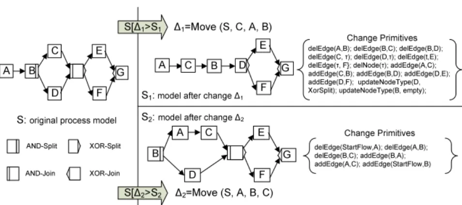
After showing the importance of changes, in this section we discuss why we need high level change operations rather than change primitives (i.e. low-level changes at edge and node level). Left side of Figure 2 shows original process model S which consists of a parallel branching, a conditional branching and a silent activityτ (depicted as empty node) connecting these two blocks. Assume that two high-level change operations are applied toS resulting in two models S1, S2: ∆1 moves activity C from its current location to the position between activitiesAandB, which leads toS1 (i.e.S[∆1iS1with ∆1=move(S,C,A,B));
∆2 moves activity A to the position between activities B and C, i.e. S[∆2iS2
with∆2=move(S,A,B,C). Figure 2 additionally depicts the change primitives, representing snapshot differences between the model S and the modelsS1 and S2, respectively.
receive treatment Admitted
a) S: original process model b) S’: final execution & change
1
3
2
4
register pay
register
receive treatment
pay
AND-Split
AND-Join
1 A possible execution order Admitted
Fig. 1.change log and execution log is not interchangeable
VI
delEdge(StartFlow,A); delEdge(A,B);
delEdge(B,C); addEdge(B,A);
addEdge(A,C); addEdge(StartFlow,B) delEdge(A,B); delEdge(B,C); delEdge(B,D);
delEdge(C, τ); delEdge(D,τ); delEdge(t,E);
delEdge(τ, F}; delNode(τ); addEdge(A,C);
addEdge(C,B); addEdge(B,D); addEdge(D,E);
addEdge(D,F); updateNodeType(D, XorSplit); updateNodeType(B, empty);
B G A
C D
E F
D
A C
E F
B G
B
A C
D
E F
G
Change Primitives
Change Primitives
∆1=Move (S, C, A, B)
S1:model after change ∆1
∆2=Move (S, A, B, C) S[∆1>S1
S[∆2>S2
S: original process model S2: model after change ∆2
AND-Split AND-Join
XOR-Split XOR-Join
Fig. 2.high-level change operation compared with change primitive
When compared to change primitives, using high-level change operations like
’move’ or ’insert’ offers the following advantages:
1. High-level change operations, as supported by ADEPT, guarantee soundness:
i.e., the application of a high-level change operation on a sound model S results in another sound model S0 [5]. This also applies to our example from Figure 2. By contrast, when applying one single change primitive (e.g.
deleting an edge inS), soundness cannot be guaranteed anymore. Generally, if we delete any of the edges in S, the resulting process model will not be necessarily sound.
2. High-level change operations provide richer syntactical meanings than change primitives. Generally, a high-level change operation is built upon a set of change primitives which collectively represent a semantic modification of a process model. As example, take∆1 from Figure 2. This high-level change operation requires 15 change primitives for its realization (deleting edges, adding edges, deleting the silent activity, and updating the node types).
3. An important aspect, not discussed so far, concerns the number of change operations needed to transform a process modelS into a target model S0. For example, we need onlyonemove operation to transformSto eitherS1or S2. However, when using change primitives, migrating S to S1 necessitates 15 changes, while the second change∆2can be realized based on 6 change primitives. This simple example shows that change primitives do not provide an adequate means to determine the difference between two process models.
Thus the number of the change primitives cannot represent the efforts for process model transformations.
3.3 The Challenge to Derive High-level Change Operations
After sketching the benefits coming with high-level change operations, this sec- tion discusses challenges of Deriving them. When comparing two process models,
VII
S’(∆1>S’’
S(∆1>S’
∆1= Delete (S, B)
∆2= Delete (S’, C)
delEdge(A,B), delEdge(B,C), addEdge(A,C), delNode(B)
delEdge(C,D), addEdge(A,D), delEdge(A,C), delNode(C) S(σ>S’’
σ =< Delete (S, B), Delete (S, C) >
delEdge(A,B), delEdge(B,C), delEdge(C,D), addEdge(A,D), delNode(B) delNode(C)
S’’ A D
S’ A C D
S A B C D
Fig. 3.undetectable change primitives
the change primitives needed for transforming one model into another can be easily determined by performing two snapshots and a delta analysis on them [1]. An algorithm to minimize the number change primitives has been given in [11]. However, when trying to derive the high-level change operations needed for model transformation, several challenges occur. Consider Figure 3 as example:
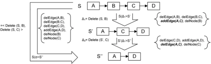
1. When performing two delete operations on S, i.e. ∆1 = delete(S,B) and
∆2 = delete(S,C), we obtain a new model S00 with S[σiS00 with σ =<
∆1, ∆2 >, as well as an undetectable intermediate model S0 with S[∆1iS0 andS0[∆2iS00. When examining the change primitives corresponding to each high-level change operation, we need to first add edge (A,C) after the first delete operation ∆1, and remove this edge (A,C) when applying the sec- ond delete operation ∆2. However, when performing a delta analysis for the original process modelS and the resulting process model S00, the two change primitives (addEdge(A,C) introduced by the first delete operation and delEdge (A,C) introduced by the seconddelete operation) jointly have no effect on the resulting process modelS00so that they cannot be detected by snapshot analysis. Consequently, deriving high-level change operations from change primitive would be challenging because the change primitives required for every high-level change will not always appear in the snapshot differences between the original and resulting models (like in Figure 3, none of the two sets of change primitives associated to∆1 or∆2 are a sub-set of the set of change primitives associated withσ).
2. Even when there is just one high-level change operation, it remains difficult to derive it with a delta algorithm. For example, in Figure 3, the delta algorithm shows that when transformingS toS1,15 change primitives need to be applied to the original modelS. However, the depicted change can be also realized by just applying one high level move operation toS.
VIII
4 Detecting The Minimal Number Of High-level Change Operations
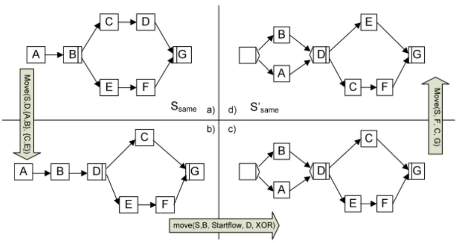
In this section, we introduce our method to detect the minimal number of change operations needed to transform a given process modelSinto another model S0. As example, consider the process modelsS andS0 in Figure 4.
4.1 General Description of our Method
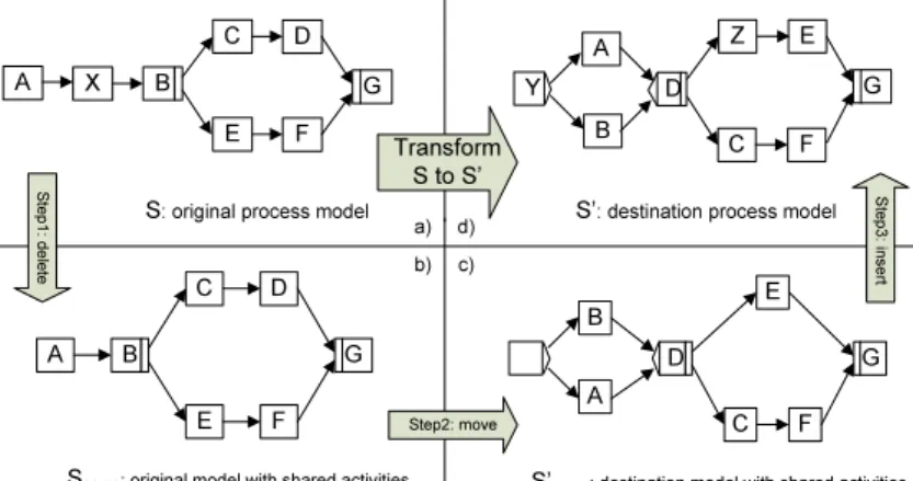
As mentioned in Section 1, the key issue of this work is to minimize the number of change operations needed to transform a process model S to another model S0. In this context, let N and N0 be the two sets of activities based on which S and S0 are defined. Generally, three steps are needed (cf. Figure 4) to realize this minimal transformation:
1. ∀ai ∈ N \N0: delete all activities being present in S, but not in S0. As depicted in our example from Figure 4, this first step transformsS toSsame
(cf. Figure 4b).
2. ∀ai ∈ NT
N0: move all activities being present in both models to the lo- cations as reflected byS0. As depicted in our example from Figure 4, this second step transformsSsame to Ssame0 (cf. Figure 4c).
3. ∀ai ∈ N0 \N: insert those activities being present in S0, but not S. As depicted in Figure 4, the third step transformsSsame0 toS0 (cf. Figure 4d).
Insertions and deletions deal with changes of the set of activities and we can hardly do anything here to reduce efforts (i.e. the number of required high-level insert/delete operations): New activities (ai ∈N0\N) must be added and ob- solete activities (aj ∈ N \N0) must be deleted. The focus of minimality can therefore be shifted to the use of themove operation, which changes the struc- ture of a process model, but not its set of activities. Since a move operation logically corresponds to a delete followed by an insert operation, we can trans- formSsame toSsame0 by maximaln=|NT
N0|move operations. Reason is that nmove operations correspond to deleting all activities and then inserting them back to their new positions. Sonwould be the maximal number of change oper- ations needed to transform one process model into another, with the same set of activities (Ssame andS0samein our example from Figure 4). However, this would be not in line with our goal of minimality. To measure the complete transforma- tion fromS toS0, we formally defineprocess distance andprocess similarity as follow:
Definition 2 (Process distance & process similarity.).
Let S, S0 ∈ P be two process models. Let N and N0 be two sets of activities based on whichS andS0 are defined. Let furtherσ=h∆1, ∆2, . . . ∆ni ∈ C∗ be a sequence of change operations transformingS intoS0 (i.e.S[σiS0). Then the dis- tance betweenSandS0 is given byd(S,S0)=min{|σ| |σ∈ C∗∧S[σiS0}. Further- more, the process similarity betweenSandS0then equals to1−|N|+|Nd(S,S0|−|N0)T
N0|. i.e. the similarity equals ((maximal number of changes - minimal number of changes) / maximal number of changes).
IX
4.2 Determining Required Activity Deletions and Insertions
To accomplish Step 1 and Step 3 of our method, we have to deal with the change of the activity set when transformingS to S0. It can be easily detected by applying existing snapshot algorithms [1] to both S andS0. As described in Section 4.1, as first step we need todelete all activitiesai ∈N\N0 contained in S, but not inS0. Regarding our example from Figure 4, we therefore can derive as our first high-level change operation ∆1 = delete(S,X). Similarly, activities contained inS0, but not inS, are to be inserted in Step 3 of our method, after we moved the shared activities to their respective position inS0(Ssame0 respectively).
The parameters of the insert operation, i.e. the predecessors and successors of the inserted activity, are just like how they appear inS0. In this way, we obtain the last two change operations for our example:Insert(S,Y,StartFlow,{A,B}) andInsert(S,Z,D,E).
4.3 Determining Required Move Operations to Deal With Structure Changes
In this section, we focus on Step 2 of our method, i.e. to transform two process models with same activity set using move operations. Here, we can ignore the activities not contained in both S and S0 (they have already been handled in Section 4.2). We therefore consider the two process models Ssame and Ssame0 respectively, as depicted in Figure 4.
Determine the Order Matrix of a Process Model One key feature of the ADEPT change framework is to maintain the structure of the unchanged parts of a process model [5]. For example, if we delete an activity, this will neither influence the successors nor the predecessors of this activity, and also not their control relationships. To incorporate this feature in our approach, rather than
S: original process model S’: destination process model E D
B C
A Z
F Y G
C
E X
D
F B G
A
C
E A
D
F G B
Ssame: original model with shared activities S’same: destination model with shared activities A
C
B E
F G D
Ste p1: d elete
Transform S to S’
Step2: move
Ste p3: in sert
a) b) c)d)
Fig. 4.Three steps to transformS intoS0
X
only looking at direct predecessor successor relationships between two activities (i.e. control flow edges), we consider the transitive control dependencies between all pairs of activities; i.e. for every pair of activities ai, aj ∈NT
N0, ai 6= aj, their execution order compared to each other is examined. Logically, we check the execution orders by considering all traces a process model can produce. The results can be formally described in a matrix An×n with n = |NT
N0|. Four types of control relations can be identified (cf. Def. 3):
Definition 3 (Order Matrix). Let S ∈ P be a process model with N = {a1, a2, . . . , an}. Let further TS denote the set of all traces producible on S.
Then, matrix An×n is called order matrix of S with Aij representing the rela- tion between different activitiesai,aj∈N iff:
– Aij = ’1’ iff (∀t∈ TS with ai, aj∈t⇒t(ai ≺aj))
If for all traces containing activities ai and aj, activity ai always appears BEFOREaj, we will denoteAij as ’1’, i.e.,ai is a predecessor ofaj in the flow of control.
– Aij = ’0’ iff (∀t∈ TS with ai, aj∈t⇒t(aj ≺ai))
If for all traces containing activity ai and activity aj, activity ai always appears AFTER aj, then we will denoteAij as a ’0’, i.e.ai is a successor ofaj in the flow of control.
– Aij = ’*’ iff (∃t1 ∈ TS, with ai, aj ∈ t1∧t1(ai ≺ aj)) ∧ (∃t2 ∈ T, with ai, aj∈t2∧t2(aj≺ai))
If there exists at least one trace in which ai appears before aj and at least one other trace in whichai appears after aj, we will denote matrix element Aij as ’*’, i.e.ai andaj are contained in different parallel branches.
– Aij = ’-’ iff (¬∃t∈ TS :ai∈t∧aj ∈t)
If there exists no trace containing both activity ai and aj, we will denote Aij as ’-’, i.e.ai andaj are contained in different branches of a conditional branching.
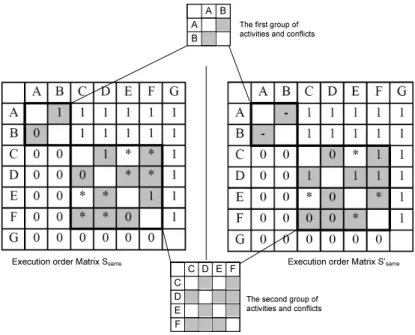
We re-visit our example from Figure 4. The order matrices of Ssame andSsame0 are shown in Figure 5. The main diagonal is empty since we do not compare an activity with itself. As one can see, elements Aij and Aji can be derived from each other. If activity ai is a predecessor of activityaj, (i.e. Aij = 1), we can always conclude that Aji = 0 holds. Similarly, if Aij ∈ {’*’,’-’}, then we will obtain Aji =Aij. As a consequence, we can simplify our problem by only considering the upper triangular matrixA= (Aij)j>i.
Under certain constraints, an order matrix A can uniquely represent the process model, based on which it was built on. This is stated by Theorem 1.
Before giving this theorem, we need to definesubstring of trace:
Definition 4 (Substring of trace).
Let t and t0 be two traces. We define t a sub-string of t0 iff [∀ai, aj ∈ t, t(ai≺aj)⇒ ai,aj ∈t0∧t0(ai≺aj)] and [∃ak ∈N:ak ∈/ t∧ak∈t0].
Theorem 1. Let S, S0 ∈ P be two process models, with same set of activities N = {a1, a2, . . . , an}. Let further TS, TS0 be the related trace sets and An×n,
XI
A0n×n be the order matrices ofS andS0. ThenS6=S0 ⇔A6=A0, if (¬∃t1, t01∈ TS:t1 is a substring oft01) and (¬∃t2, t02∈ TS0:t2 is a substring oft02).
According to Theorem 1, a process modelS and order matrix A is a one- to-one mapping if the substring constraint is satisfied. A detailed discussion of the sub-string restriction is given further in Section 4.4. A proof of Theorem 1 can be found in [27]. Thus, when comparing two process models, it is sufficient to compare their order matrices (cf. Def. 3), since a order matrix can uniquely represent the process model. This also means that thedifferences of two process models can be related to thedifferences of their order matrices. If two activities have different execution order in two process models, we define the notionconflict as follows:
Definition 5 (Conflict).. LetS, S0 ∈ Pbe two process models with same set of activitiesN. Let furtherAandA0 be the order matrices forSandS0 respectively.
Then: Activitiesaiandaj are conflictingiffAij 6=A0ij. We formally denote this as C(ai,aj). CF := {C(ai,aj) | Aij 6= A0ij}, then corresponds to the set of all existing conflicts.
Figure 5 marks up differences between our two order matrices in grey. The set of conflicts is as follows: CF = {C(A,B), C(C,D), C(C,F), C(D,E), C(D,F), C(E,F)}.
Optimizing the Conflicts To come fromSsametoSsame0 , we have to eliminate conflicts between them by applying move operations. Obviously, if there is no
Execution order Matrix Ssame Execution order Matrix S’same
A B A B
The first group of activities and conflicts
C D E F C
D E F
The second group of activities and conflicts
Fig. 5.the execution order matrices ofSsameandSsame0 in Figure 4
XII
conflict for the two process models Ssame andS0same, they are identical. Every time we move an activity from its current position inSsameto the position it has inSsame0 , we can eliminate the conflicts this activity has with other activities. For example, consider activityAin Figure 4. If we move activityAfrom its position in Ssame (preceding B) to its new position in Ssame0 (Aand B are contained in two different branches of a conditional branching block), then we can eliminate conflict C(A,B). Shown in the order matrices, moving activity A requires two steps. First, set the elements in the first row and first column of An×n (which corresponds to activity A) to empty, sinceAis moved away. Second, reset these elements according to the new order relation of A, when compared to the other activities fromSsame0 . So every time we move an activity, we are able to change the value of its corresponding row and column in the order matrices, i.e., we change these values corresponding to the original model to the values compliant with the target model. By doing this iteratively, we can change all the values and eliminate all the conflicts so that we could achieve the transformation from Ssame to Ssame0 .
A none-optimal solution to transform the processes would be to move all the activities contained in the conflicts inCF, from their positions in Ssame to the positions they have in Ssame0 . Regarding our example from Figure 5, to apply this straightforward method, we would need to move activitiesA,B,C,D,EandF from their positions inSsame to the ones inSsame0 . However, this naive method is not in line with our goal to minimize the number of applied change operations.
For example, after moving activity A from its current position in Ssame to the position it has inSsame0 , we do not need to move activity B anymore, because after this change operation, there are no activities with which activityBstill has conflicts.
Digital logic in Boolean algebra [20] helps to solve this minimization prob- lem. Digital logic constitutes the basis for digital electronic circuit design and optimization. In this field, engineers face the challenge to optimize the internal circuit design given the required input and output signals. To apply such a tech- nique in our context, we consider each process activity as an independent input signal and we want to design a circuit which can cover all conflicts defined byCF (cf. Def 5). If activityai conflicts to activityaj, we can either move one of them or both of them from the positions they have in Ssame to the ones they have in Ssame0 . Doing so, the conflict will not exist any more. Reason is that every time we move an activity from the position it has in Ssame to the position it has inSsame0 , we reset the corresponding row and column of this activity in the order matrix. A conflict can be interpreted as a digital signal as follows: when the two input signals ai and aj are both ”true”(this means we do not move activity ai and aj), we cannot solve the conflict and the ’circuit’ shall give an output signal of ”false”, (i.e.aiaj = 0). If we apply this to all conflicts inCF, we will obtain all the ”false” signals. Meanwhile, the ”circuit” should be able to tell us what will result in a ”true” output, (i.e. the negative of all ”false” signals).
This ”true” output represents which activities we need to move. Regarding our
XIII example from Figure 5, given the set of conflicts CF, our logic expression then is:AB+CD+CF+DE+DF+EF.
The complexity for optimizing the logic expression is NP-Hard [20]. Therefore it is advantageous to reduce the size of the problem. Concerning our example, we can cut down the optimization problem into two groups: one with activitiesA andB, and conflictC(A,B); another one with activitiesC,D,EandFand conflicts {C(C,D),C(C,F),C(D,E),C(D,F),C(E,F)}.
Such a division can be achieved inO(n) time in the following three steps. Step 1: List all the conflicting activities, and set every activity as a group. Step 2: If conflicting activitiesaiandaj(i.e.C(ai,aj)) are contained in two different groups, merge these two groups. Step 3: Repeat Step 2 for all conflicts inCF. After these three steps, we can divide the activities as well as the associated conflicts into several groups. Regarding our example, the optimization problem can be divided into two sub-optimization problems:ABandCD+CF+DE+DF+EF. We depict this in the two small matrices in Figure 5.
Optimizing logic expression has been discussed intensively in Discrete Math- ematics. Therefore we omit details here and refer to Karnaugh map [20] and Quine-McCluskey algorithm [20]. We have implemented the latter in our proof- of-concept prototype. Regarding our example in Figure 4, the two optimiza- tion results are: AB = ¯A+ ¯B for the first group, and CD+CF+DE+DF+EF=
¯D¯F+ ¯C¯E¯F+ ¯CD¯¯E for the second group. We can interpret this result as follows.
For the second group, either we move activities Dand F, or we move activities C,EandF, or we move activitiesC,DandEfrom their position inSsame to the positions they have inS0same. Based on this, we can transformSsame toS0same, since all conflicts are eliminated. As can be seen from the order matrices, if we change the value of the corresponding rows and columns of these activities in Ssame, we can turn Ssame into S0same. As we want to minimize the number of change operations, we can draw the conclusion that activities D andF must be moved. Same rule applies to the result of the first group. However, there is no difference to move either Aor B, since both operations count as one change operation. Here, we arbitrarily decide to move activity B.
So far we have determined the set of activities to be moved. The next step is to determine the positions where the activities need to be moved to. Operation move(S,X,A,B,[sc]) will be independent from other move operations (i.e. it does not matter in which order to move the respective activity) if its direct predecessors A and direct successors B do not belong to the set of activities to be moved. Regarding our example from Figure 4, activity F satisfies this condition since its predecessorCand successor Gare not moved. If this had not been the case, we would have to introduce silent activities to put the moved activity to its corresponding place in Ssame0 . For example, if we want to first moveBto its position inSsame0 , we will have to introduce a silent activity after Band beforeCandE. Only in this way, we can change the execution order of B to what it appears inSsame0 . However, such silent activity will be not required if we first move activityDto the position it has in Ssame0 . A detailed discussion
XIV
C
E A
D
F G B
Ssame S’same
Mov e(S,D ,{A,B }, {C ,E})
move(S,B, Startflow, D, XOR)
Mov e(S, F , C, G ) a)
b) c) d)
A
C
B E
F G D
A
E
B C
F G D
C
E
A B
F G D
Fig. 6.Process models after every move operation
is out of the scope here; we refer readers to the reduction rules introduced with the ADEPT method [5].
According to the position the moved activities have inSsame0 , we can deter- mine the parameters (i.e. the predecessors, successors and conditions) for every move operation. InSsame0 , activity Dhas predecessorsAandB, and successorsE andC. So one move operations therefore is:move(S,D,{B,A},{C,E}). Similarly, we obtain the other two move operations: move(S,B,StartFlow,D,XOR) and move(S,F,C,G). The intermediate process models resulting after every move op- eration is shown in Figure 6. When comparing order matrices for each model in Figure 6, it becomes clear that every move operation changes the values of the row and the column corresponding to the moved activity.
4.4 Silent Activities
A silent activity is an activity which does not contain any operation or action, and which only exists for control flow purpose. There are two reasons why we do not consider silent activities in our similarity measure:
1. The appearance of a silent activity can be random. We can add or remove silent activities without changing the behavior of the process model. For example, we can replace a control flow edge in a process model by one silent activity or even a block of silent activities without influencing the behavior of the process model.
2. The existence of a silent activity also depends on other activities and is subject to change as other activities change. As example consider Figure 2.
When applying change operation∆1toS, the silent activityτ is automati- cally removed after activityCis moved away.
However, there is one exception for which we need to consider silent activities.
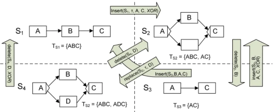
Consider the two process modelsS1andS2as depicted in Figure 7. If we ignore
XV
TS2= {ABC, AC}
TS1 = {ABC}
S2
S1 A B C A C
B
A C
B
D TS3 = {AC}
S3
S4 A C
TS2= {ABC, ADC}
Insert(S1, τ, A, C, XOR)
dele te(S 4, D , XO R)
delete(S4, D) replace(S2, τ, D)
dele te(S 2, B)
inse rt(S3 , B ,
A, C , XO R) Insert(S3,B,A,C)
Fig. 7.The influence of silent activity
the silent activity τ (depicted as an empty node) in S2, and derive the order matrix of process modelS2, it will be the same as the one ofS1. Obviously, the two process model are not equivalent since the trace sets producible by them are not identical. More precisely, TS2 contains one additional trace when compared to TS1. In general, if one process model can produce additional traces, which are the sub-string of other traces (cf. Def.4), there must be some silent activities we cannot ignore. Or if the direct predecessor and direct successor of one silent activity constitute XORsplit and XORjoin, we can also not ignore this silent activity (cf.S2 in Figure 7).
Figure 7 shows several process model transformations based on high level change operations. Here we can identify the difference between the two types of deletion: delete(S4,D) anddelete(S4,D,XOR) (cf. Figure 7). The former one turns an activity into a silent one (transforming S4 into S2), while the latter one blocks the branch which contains activity D(transforming S4to S1). When a branch is blocked, we do not allow the activities of the branch to become activated [14, 5]. Since process modelsS1andS2have same order matrix, purely comparing order matrices (cf. Section 4) would not be sufficient in the given situation. Reason is that an order matrix does not uniquely represent a process model, since the sub-string constraint (cf. Def.4) in Theorem 1 is violated. To extend our method such that it can uniquely represent a process model without the sub-string constraint, we must consider these special silent activities (i.e.
a silent activity which has direct predecessor of XORsplit and direct successor of XORjoin) as well. They will appear in the order matrix and their execution orders compared with other activities will be documented.
However, the existence of a silent activity is still very much dependent on other activities, including the scenario described above. For example, if we delete activity B in S2 as depicted in Figure 7, we will transform S2 into S3, i.e. the silent activity will be simultaneously deleted when activityBis deleted. We can identify this situation by either examining the process model or the order matrix.
In the process model, a silent activityτ can be automatically deleted if there is another silent activity τ0 which is contained in the same block but in another
XVI
Figure 2 Figure 4
S S1 S2 S Ssame S'same S'
S 0 / 100% 1 / 86% 1 / 86% 4 / 50% 3 / 57% 3 / 57% 5 / 44%
Figure 2 S1 0 / 100% 2 / 71 % 4 / 50% 3 / 57% 3 / 57% 5 / 44%
S2 0 / 100% 5 / 38% 4 / 42% 3 / 57% 5 / 44%
S 0 / 100% 1 / 88% 4 / 50 % 6 / 40%
Figure 4 Ssame 0 / 100% 3 / 57% 5 / 44%
S'same 0 / 100% 2 / 78 %
S' 0 / 100%
Fig. 8.The distances and similarities of different process models
conditional branch (e.g. transforming S2 to S3 Figure 7). In the order matrix, we can automatically remove a silent activityτ if there is another silent activity τ0 which has the same order relations to the rest of the activities asτ has.
In general, when a silent activity has an XORsplit as direct predecessor and an XORjoin as direct successor, we need to consider this silent activity when computing the order matrix of a process model. However, these silent activities can automatically been deleted when changing the process model. This requires us to perform additional checks on the process model or order matrix (as de- scribed above) after every change operation.
4.5 Summary
Taking our example from Figure 4, to transform S into S0 (S[σiS0), the fol- lowing six change operations are required: σ = {delete(S,X), move(S,F,C,G),
move(S,D,{A,B},{C;E}),move(S,B,StartFlow,D,XOR),insert(S,Y,StartFlow,{A,B}), insert(S,Z,D,E)}. The distance between the two process models issix, and the
similarity is0.4 (cf. Def.2).
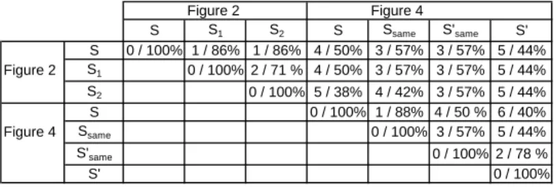
To illustrate our method and these numbers in more detail, we compare the distances and similarities between seven process models discussed so far:S, S1
andS2 in Figure 2 as well as S,Ssame, Ssame0 andS0 in Figure 4. The distance and similarity of two process models are specified asdistance/similarityin each corresponding cell in Figure 8. As the transformation is commutable, we only fill in the upper triangle matrix. Taking Figure 8, we can conclude the following:
1. Changing the activity set always leads to changing distance. For example, d(Sn,S0same) always equalsd(Sn,S0)+ 2, whereSn stands for a process model other thanS0 orS0same in Figure 8. Reason is that S0 contains two unique activitiesYandZwhen compared toSsame0 , while the rest are identical.
2. If three process modelsS,S0, andS00have the same set of activities,d(S,S00)≤ d(S,S0)+d(S0,S00) will hold. It is also easy to understand this because some activities could be moved twice when transformingSintoS0andS0intoS00.
XVII
5 related work
Various papers have studied the process similarity problem and provided some useful results [12–14, 21]. In graph theory, graph isomorphism[2] and sub-graph isomorphism [24] are often used to measure the similarity between two graphs.
Unfortunately, these measures usually only examine edges and nodes and cannot catch the syntactical issues of a PAIS. In the database field, the delta-algorithm [1] is used to measure the difference between the two models. It extends the above mentioned approaches by assigning attributes to edges and nodes [11].
Still, it can only catch change primitives, and will further run into problems when catching the high-level change operations (as described in Section 3). In the fields of Petri-nets and state automata, similarity based on change is difficult to measure since these formalisms are not very tolerant for changes. Inheritance rules [14] are one of the very few techniques given to show the transformation of a process model described as Petri-net. Trace equivalence is commonly used to compare whether two process models are similar or identical [26]. In addition, bisimulation [14, 15] extends trace equivalence by considering stronger notions.
Also based on traces, [12] assign weights to each trace based on execution logs which reflect the importance of a certain trace. Respective techniques are applied, for example in genetic process mining [13]. The edit distance [21] is also used to measure the difference between traces; the sum of them represents the differences of two models. Some similarity measures use two figures (precision and recall) to evaluate the difference between process models S1 to S2 [12, 16]. However, this asymmetric way might lead confusion since it is therefore not commutable.
None of these approaches measures the similarity by a unique and commutative figure, based on the effort for change.
6 Summary and OutLook
We have provided a method to quantitatively measure the distance and similarity between two process models based on the efforts for model transformation. High- level change operations are used to evaluate the similarity since they guarantee soundness and also provide more meaningful results. We further applied digital logic in boolean algebra so that the number of change operations required to transform process modelS into process modelS0 is minimized.
Some additional work is needed to enrich our knowledge on process similar- ity. As a first step, we will extend our method so that it will be able to measure the similarity between process models using additional constitutes (e.g., syn- chronization and loopback edges [5]). The next step will be to incorporate data flow, temporal constraints, and resources, so that the similarity measure can be further applied to practice.
References
1. W.Labio , H.Garcia-Molina: Efficient Snapshot Differential Algorithms for Data Warehousing. 22th Int. Conf. on Very Large Data Bases. pp 63-74, 1996
XVIII
2. L.Babai ,P.Erd¨os, S.M.Selkow: Random Graph Isomorphism. SIAM Journal of Computation 9, pp 628-634, 1980
3. P.Balabko, A.Wegmann, A.Ruppen and N.Clement: Capturing design rationale with functional decomposition of roles in business processes modeling. Software Process: Improvement and Practice. 10(4):379-392, 2005.
4. I Bider: Masking flexibility behind rigidity: Notes on how much flexibility people are willing to cope with. CAiSE’05 Workshop, pp 7-18, 2005.
5. M. Reichert and P. Dadam.ADEPTflex - Supporting Dynamic Changes of Work- flows Without Losing Control. Journal of Intelligent Information Systems, 10(2):93–
129, 1998.
6. M.Dumas, W.M.P. van der Aalst, and A.H.M. ter Hofstede: Process-Aware Infor- mation Systems: Bridging People and Software through Process Technology. Wiley
& Sons, 2005.
7. S.Rinderle, M.Reichert and P.Dadam. Correctness Criteria for Dynamic Changes in Workflow Systems - A Survey. Data and Knowledge Engineering, 50(1):9-34, 2004.
8. S.Rinderle, B.Weber, M.Reichert and W.Wild:Integrating Process Learning and Process Evolution-A Semantics Based Approach. BPM’05, pp 252-267,2005.
9. M.Kradolfer and A.Geppert:Dynamic workflow schema evolution based on work- flow type versioning and workflow migration. CoopIS’99, pp 104-114, 1999 10. M.Weske: Formal foundation and conceptual design of dynamic adaptations in a
workflow management system. HICSS-34, 2001.
11. S.Rinderle, M.Jurisch and M.Reichert:On Deriving Net Change Information From Change Logs CThe DELTA-LAYER Algorithm. BTW’07, pp364-381,2007 12. W.M.P. van der Aalst, A.K. Alves de Medeiros, and A.J.M.M. Weijters: Pro-
cess Equivalence: Comparing Two Process Models Based on Observed Behavior.
BPM’06, LNCS 4102, pp 129-144. 2006.
13. A.K.A. de Medeiros, A.J.M.M. Weijters and W.M.P. van der Aalst.Genetic Process Mining: A Basic Approach and its Challenges. BPM’05 Workshops , LNCS 3812 pp 203-215. 2006.
14. W.M.P. van der Aalst and T. Basten:Inheritance of Workflows: An Approach to Tackling Problems Related to Change. Theoretical Computer Science, 270(1-2):125- 203, 2002
15. R.J. van Glabbeek and W.P. Weijland:Branching Time and Abstraction in Bisim- ulation Semantics.Journal of the ACM, 43(3):555-600, 1996.
16. S.S. Pinter and M. Golani:Discovering Workflow Models from Activities’ Lifespans.
Computers in Industry, 53(3):283-296, 2004.
17. C.W. G¨unther, S. Rinderle, M. Reichert, and W.M.P. van der Aalst: Change Mining in Adaptive Process Management Systems. CoopIS’06, LNCS 4275, pp 309-326. 2006.
18. M.Reichert, S.Rinderle and P.Dadam: On the common support of workflow type and instance changes under correctness constraints. CoopIS’03, LNCS 2888, pp 407-425, 2003.
19. T.H.Cormen, C.E.Leiserson, R.L.Rivest and C.Stein: Introduction to Algorithms, Second Edition. MIT press, 2001, pp 549-552
20. S.Brown and Z.Vranesic: Fundamentals of Digital Logic with Verilog Design.
McGraw-Hill, 2003
21. A.Wombacher and M.Rozie:Evaluation of Workflow Similarity Measures in Service Discovery. Service Oriented Electronic Commerce. pp 51-71, 2006
22. S.Rinderle:Schema Evolution in Process Management Systems. Ph.D thesis, Univ.
of Ulm, 2004
XIX
23. D.M. Strong and S.M. Miller:Exceptions and exception handling in computerized information processes. ACM Trans on Information Systems, 13(2):206-233, 1995 24. E. B.Krissinel and K.Henrick:Common subgraph isomorphism detection by back-
tracking search. Softw. Pract. Exper. 34(6):591-607, 2004
25. B.Weber and S.B.Rinderle and M.Reichert:Change Patterns and Change Support Features in Process-Aware Information Systems. CAiSE 2007, LNCS 4495. pp 574- 588. 2007
26. J.Hidders, M.Dumas, W. M.van der Aalst, A. H. ter Hofstede, and J.Verelst.When are two workflows the same?. 2005 Australasian Symposium on theory of Comput- ing - Vol 41. ACM vol. 105. 3-11. 2005
27. C.Li, M.Reichert, A.Wombacher.Process Similarity Based on High Level Change Operations. CTIT Technical Report, University of Twente, The Netherlands.