Analyzing the Impact of Process Change Operations on Time-Aware Processes
Andreas Lanz∗, Manfred Reichert∗
Institute of Databases and Information Systems, Ulm University, Germany
Abstract
The proper handling of temporal process constraints is crucial in many application domains. Contemporary process-aware information systems (PAIS), however, lack a sophisticated support of time-aware processes.
As a particular challenge, the enactment of time-aware processes needs to be flexible as time can neither be slowed down nor stopped. Hence, it should be possible to dynamically adapt time-aware process instances to cope with unforeseen events. In turn, when applying such dynamic changes, it must be re-ensured that the resulting process instances aretemporally consistent; i.e., they still can be completed without violating any of their temporal constraints. This paper extends existing process change operations, which ensure soundness of the resulting processes, with temporal constraints. In particular, it provides pre- and post-conditions for these operations that guarantee for the temporal consistency of the changed process instances. Further, we analyze the effects a change has on the temporal properties of a process instance. In this context, we provide a means to significantly reduce the complexity when applying multiple change operations. The presented change operations have been prototypically implemented in the AristaFlow BPM Suite.
Keywords: time-aware processes, dynamic process change, process flexibility, process-aware information system
1. Introduction
Time is a crucial factor regarding the support of various business processes [1]. Moreover, in many application areas (e.g., patient treatment, automotive engineering), the proper handling oftemporal constraints is vital in order to successfully execute and complete processes [2, 3, 1]. However, contemporary process-aware information systems (PAIS) lack a more sophisticated support of suchtime-aware business processes[1]. To remedy this drawback, the proper integration of temporal constraints with both the design and run-time components of a PAIS has been identified as a key challenge [2, 3, 4].
As a prerequisite for robust process execution in PAISs, the executableprocess models must besound [5].
Moreover, in the context oftime-aware process models, i.e., process models enriched with temporal constraints, theconsistency of the temporal constraints must be ensured [6, 3, 4]. Checking consistency of time-aware process models at design-time has been extensively studied in literature [6, 2, 7]. By contrast, only little attention has been paid to the proper run-time support of time-aware processes [4]. During run-time, the temporal consistency of process instances needs to be continuously monitored and re-checked to avoid constraint violations. Particularly, note that activity durations and deadlines may be specific to the enacted process instance and solely become known during run-time [4].
As a particular challenge, temporal constraints cannot be considered in isolation, but might interact with each other. Hence, complex algorithms are required for checking the temporal consistency of a process model [4, 8]. However, at run-time respective calculations should be reduced to a minimum to ensure
∗Corresponding author
Email addresses: andreas.lanz@uni-ulm.de(Andreas Lanz),manfred.reichert@uni-ulm.de(Manfred Reichert)
scalability of the PAIS [4]. Otherwise, a run-time support of time-aware processes will not be possible at the presence of a large number of process instances.
As another challenge, time can neither be slowed down nor stopped. Accordingly, time-aware processes need to beflexibleto cope with unforeseen events or delays during run-time [9]. For example, it is common that deadlines are re-scheduled or temporal constraints are dynamically modified in order to successfully complete a process instance being in trouble. Moreover, in certain scenarios the instances of time-aware processes must be structurally changed (e.g., by moving, deleting, or inserting activities) to be able to meet a particular deadline. In the context of suchdynamic process changes, we must re-ensure that the resulting process instances are sound and temporally consistent. While soundness has been extensively studied in literature [10, 11, 5], this work shows how temporal consistency of a time-aware process instance can be efficiently ensured in the context of dynamic changes. Furthermore, we analyse the effects, changes have on the temporal constraints of the respective process instance. In particular, we show how the results of this analysis can be utilized to significantly reduce the complexity when applying multiple change operations. For example, the latter becomes crucial in the context of process evolution, where a possibly large set of process instances needs to be migrated on-the-fly to a changed process model [5].
The remainder of the paper is organized as follows: Section 2 considers existing proposals relevant for our work. Section 3 provides background information on time-aware processes and defines the notion of temporal consistency. Section 4 first introduces the set of change operations we consider, followed by an in-depth discussion on how these change operations work in the context of time-aware processes. Section 5 analyzes the impact a change has on the temporal constraints of a process and proposes useful optimizations.
Section 6 evaluates the proposed approach. Finally, Section 7 concludes with a summary and outlook.
2. Related Work
In literature, there exists considerable work on managing temporal constraints for business processes [6, 2, 7, 4, 12]. The focus of these approaches is on design-time issues like the modeling and verification of time-aware processes. By contrast, only few approaches consider execution issues of time-aware processes [3, 4].
In particular, none of the latter considers dynamic changes in this context.
Most approaches dealing with the verification of time-aware processes use a specifically tailored time model to check for the temporal consistency of process models. This becomes necessary since the interdependencies between the various temporal constraints of a process model can be quite complex and cannot be suitably captured in the respective process model. A specific conceptual model for temporal constraints is defined in [12]. In turn, [3, 7] use an extended version of the Critical Path Method (CPM) known from project planning. Simple Temporal Networks(STN) are used in [6] as basic formalism, whereas [4] suggests using Conditional Simple Temporal Networks with Uncertainty for checking the controllability of process models, i.e., a more restrictive form of temporal consistency. This paper relies on Conditional Simple Temporal Networks(CSTN), an extension of STN that allows for the proper handling of exclusive choices [8].
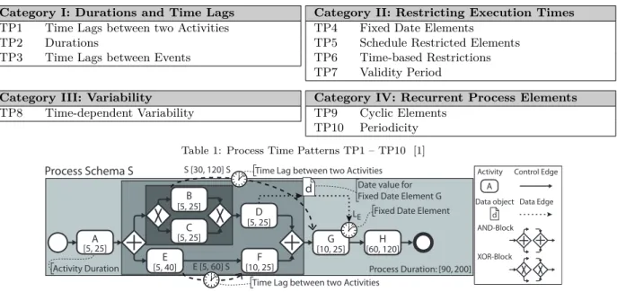
In [1], we presented 10 empirically evidenced time patterns (TP), that represent temporal constraints relevant in the context of time-aware processes (cf. Table 1). In particular, time patterns facilitate the comparison of existing approaches based on a universal set of notions with well-defined semantics [13].
Moreover, [13, 1] elaborated the need for a proper run-time support of the time patterns and time-aware processes.
Dynamic process changes were extensively studied in the past. Particularly, there exists considerable work on ensuring structural and behavioural soundness in the context of dynamic process instance changes [10, 11].
Further, [14] presents an overview of frequently used patterns for changing process models whose semantics is described in [11]. Finally, a comprehensive survey of approaches enabling dynamic changes is provided in [5].
To the best of our knowledge, [9] is the only work considering dynamic changes in the context of time-aware processes. As opposed to this paper, however, [9] only provides a high level discussion of the different aspects to be considered when changing time-aware process instances, temporal consistency being one of them.
Category I: Durations and Time Lags TP1 Time Lags between two Activities TP2 Durations
TP3 Time Lags between Events
Category II: Restricting Execution Times TP4 Fixed Date Elements
TP5 Schedule Restricted Elements TP6 Time-based Restrictions TP7 Validity Period
Category III: Variability TP8 Time-dependent Variability
Category IV: Recurrent Process Elements TP9 Cyclic Elements
TP10 Periodicity Table 1: Process Time Patterns TP1 – TP10 [1]
A Activity
Data object d AND-Block
XOR-Block
Control Edge
Data Edge
A
B
D C
E
H F
G Process Schema S
[5, 25]
LE S [30, 120] S
d
E [5, 60] S [5, 25]
[5, 25]
[5, 25]
[5, 40] [10, 25]
[10, 25] [60, 120]
Process Duration: [90, 200]
Fixed Date Element
Activity Duration
Date value for Fixed Date Element G Time Lag between two Activities
Time Lag between two Activities
Figure 1: Core Concepts of a Time-Aware Process Model
3. Basic Notions
This section provides basic notions. First, it defines a basic set of elements for modeling time-aware processes. Second, it introduces the concept of temporal consistency for time-ware processes.
3.1. Time-aware Processes
For each business process exhibiting temporal constraints, atime-aware process schemaneeds to be defined (cf. Figure 1). In our work, a process schema corresponds to aprocess model; i.e., a directed graph, that comprises a set ofnodes—representingactivitiesandcontrol connectors (e.g., Start-/End-nodes, XORsplits, or ANDjoins)—as well as a set of control edges linking these nodes and specifying precedence relations between them. We assume that process models are well structured [5], e.g., sequences, and branchings (i.e., parallel and exclusive choices) are specified in terms of nested blocks with unique start and end nodes of same type. These blocks—also known as SESE regions [15]—may be arbitrarily nested, but must not overlap;
i.e., their nesting must be regular [16]. Figure 1 depicts an example of a well structured process model with the grey areas indicating respective blocks. Each process model contains a unique start and end node, and may be composed of control flow patterns like [17]: sequence, parallel split (ANDsplit), synchronization (ANDjoin), exclusive choice (XORsplit), and simple merge (XORjoin) (cf. Figure 1). Note that we do not consider loops in this paper. However, in the context of time-aware processes a loop may be mapped to a set of nested XOR blocks [4].
In addition, a process model containsdata objectsas well asdata edgeslinking activities with data objects.
More precisely, a data edge either represents a read or write access of the referenced activity to the referred data object.
At run-time,process instancesmay be created and executed according to the defined process model. We assume that a process instance is logically represented by a clone of the respective process model augmented with instance-specific information. In turn, activity instancesrepresent executions of single process steps (i.e., activities) of such a process instance.
If a process model contains XOR-blocks, uncertainty is introduced since not all instances perform exactly the same set of activities. The concept ofexecution path allows us to identify which activities and control connectors are actually performed during one execution of a process instance. Particularly, given a process model, an execution path denotes a connected maximal subgraph of the process model containing its start and end node, in which all XORsplit connectors have exactly one branch. An execution path can be also briefly described by a string containing the activity identifiers of the execution path sorted with respect to
their execution order and separated by a dash if the order is sequential or by a vertical bar if it is parallel [2].
As example, considering the process model from Figure 1, the stringA-((B-D)|(E-F))-G-Hrepresents an example of an execution path, whereAis followed by a parallel execution of two sequential paths (B-D) (i.e., , for the XORsplit the upper path is selected) and (E-F); then,GandHare sequentially executed. Note that the set of execution paths may have an exponential cardinality with respect to the number of XOR blocks in the process model.
We base our work on the 10 time patterns (TP) we presented in [1] (cf. Section 2). To set a focus, this work specifically considers the patterns being most relevant in practice [1]; i.e.,time lags between two activities(TP1),durations of activities and processes(TP2), andfixed date elements of activities(TP4). In detail:
Anactivity durations(TP2) defines the minimum and maximum time span allowed for executing a particular activity (or node, in general), i.e., the time span between start and completion of the activity [1].
We assume that each activity has an assigned duration. Activity durations are described in terms of minimum and maximum values [dmin, dmax] where 0≤dmin≤dmax. Since control connectors are automatically performed, one may assume that they have a fixed duration defined by the PAIS (e.g., [0,1]).
Process durations (TP2) represent the time span allowed for executing an instance of the process model, i.e., the time span between start and completion of the process instance [1]. Again, a process duration is described in terms of minimum and maximum values [dmin, dmax] where 0≤dmin≤dmax.
Time lags between two activities(TP1) restrict the time span allowed between the starting and/or ending instants of two arbitrary activities of a process model [1]. Such a time lag may not only be defined between directly succeeding activities, but between any two activities that may be conjointly executed in the context of a particular process instance, i.e., the activities must not belong to exclusive branches. In Figure 1, a time lag is visualized through a dashed edge with a clock symbol between the source and target activity.
The label of the edge specifies the constraint according to the following template: hISi[tmin, tmax]hITi;
hISi ∈ {S, E} andhITi ∈ {S, E} mark the instant (i.e., starting or ending) of the source and target activity the time lag applies to; e.g.,hISi=S marks the starting instant of the source activity andhITi=E the ending instant of the target activity. In turn, [tmin, tmax] (−∞ ≤tmin≤tmax≤ ∞) represents the range allowed for the time span between instantshISiandhITi. In particular, time lags may be used to specify minimum delays and maximum waiting times between succeeding activities. Finally, note that a control edge implicitly represents anE[0,∞]S time lag between its source and target activity, i.e., the target activity may only be started after completing the source activity.
Fixed date elements (TP4) refer to activities and allow restricting their execution in relation to a specific date [1], e.g., a fixed date element may define that the activity must not be started before or must be completed by a particular date.1 Generally, the value of a fixed date element is specific to a process instance, i.e., it is not known before creating the process instance or even becomes known only during run time. Therefore, the respective date of a fixed date element is stored in a data object. When evaluating the fixed date element during run-time, the current value of the respective data object is retrieved [13].
Figure 1 visualizes a fixed date element through a clock symbol attached to the activity. In this context, labelhDi ∈ {ES, LS, EE, LE}represents the activity’s earliest start date (ES), latest start date (LS), earliest completion date (EE), or latest completion date (LE), respectively.
Figure 1 shows an example of a process model exhibiting temporal constraints. Even though we use the notation defined by BPMN for illustration purpose, the approach described in the following is not BPMN-specific. Further note that, although some of the symbols used for visualizing the temporal constraints resemble BPMN timer events, their semantics is quite different and should not be mixed up. As can be easily verified, in Figure 1 all activities have a corresponding activity duration. The duration of activityA, for example, expresses thatAhas a minimum duration of 5 and a maximum duration of 25. BetweenBandG there is a time lag described byS[30,120]S, i.e., between the start of Band the start of Gthere must be a minimum delay of 30 time units and a maximum waiting time of 120 time units. Additionally, there is a time lag betweenEandF. Next,Ghas a fixed date element attached to it, whereby labelLE indicates that
1Fixed date elements are often referred to as “deadlines”. However, this does not completely meet the intended semantics.
the latest end date of the activity is restricted by the temporal constraint. In turn, the date of the fixed date element is provided by activityDthrough data objectd.
3.2. Temporal Consistency of Time-Aware Processes
A time-aware process model is executed by performing its activities and control connectors, thereby obeying any structural or temporal constraints of the process model. We denote a process model as temporally consistentif it is possible to perform allexecution pathswithout violating the temporal constraints involved. Temporal consistency of a time-aware process model (as well as respective process instances) constitutes a fundamental prerequisite for its robust and error-free execution. In particular, executing a process instance whose model is not temporally consistent leads to a waste of resources [6, 3]. Therefore, for any PAIS supporting time-aware processes, a crucial task is to check temporal consistency of the process model at design-time as well as to monitor and re-check corresponding instance during run-time. This is particularly challenging since different temporal constraints might interact with each other resulting in complex interdependcies (e.g., a future deadline might restrict the duration of some or all preceding activities).
Whether or not a time-aware process model is temporally consistent can be checked by mapping it to a conditional simple temporal network (CSTN)—a problem known from artificial intelligence [8, 18]. In our work, we use CSTN since it allows us to exploit and reusechecking algorithmsfor a well founded model for representing temporal constraints. Finally, CSTN allows capturing the complex interdependencies between constraints, which cannot be suitably captured in time-aware process models.
Definition 1(Conditional Simple Temporal Network). A Conditional Simple Temporal Network(CSTN) is a 6-tuplehT,C, L,OT,O, Pi, where:2
• T is a set of real-valued variables, called time-points;
• P is a finite set of propositional letters (or propositions);
• L:T →P∗ is a function assigning a label to each time-point inT; a labelis any (possibly empty) conjunction of (positive or negative) letters fromP.3
• C is a set of labeled simple temporal constraints (constraintin the following); each constraintcXY ∈ C has the formcXY =h[x, y]XY, βi, whereX, Y ∈ T are any time-points,−∞ ≤x≤y≤ ∞are any real numbers, andβ ∈P∗ is a label.
• OT ⊆ T is a set of observation time-points;
• O:P → OT is a bijection that associates a unique observation time-point to each propositional letter fromP.
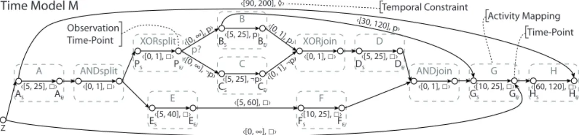
Time-points represent instantaneous events that may be, for example, associated with the start or end of activities. In turn,observation time-points represent the time point at which relevant information for the execution of the CSTN is acquired, i.e., it represents the time-point a decision regarding possible execution paths is made. More formally, when executing observation time-pointP, the truth-value of the associated proposition (i.e.,O−1(P)) is determined (observed in CSTN jargon). A constraint cXY =h[x, y]XY, βiexpresses that the time span between time-pointsX andY must be at leastxand at mosty, i.e., Y −X ∈[x, y]. Thelabel attached to each time-point and constraint, respectively, indicates the different possible executions of the CSTN, i.e., a particular time-point or constraint will be only considered if the corresponding label is satisfiable in the respective instance. Figure 2 depicts the CSTN corresponding to the process model from Figure 1.
The solution to a CSTN can be defined as follows [18]:
Definition 2 (Scenario & Solution). Given a CSTNS =hT,C, L,OT,O, Pi, a scenario over set P is a function sP :P → {true, f alse}, which assigns a truth-value to each proposition in P.
Asolution for CSTNS under scenariosP then corresponds to a complete set of assignments to all time- pointsX ∈ T withsP(L(X)) =true, which satisfies all constraintsh[x, y]XY, βi ∈ C for which sP(β) =true holds.
2For a more complete definition and a characterization see [18].
3In the following we use small Greek lettersα, β, . . .to denote arbitrary labels. The empty label is denoted by .
AS AE
FS FE
GS GE
DS DE
HS HE
ES EE
BS BE
CS CE
PS PE
Time Model M
Z
ANDsplit G H
A
B
C ANDjoin
XORsplit
p? XORjoin D
‹[5, 25], □›
‹[5, 40], □› ‹[10, 25], □›
‹[0, 1], □› ‹[0, 1], □› ‹[10, 25], □› ‹[60, 120], □›
‹[0, 1], □›
‹[5, 25], p›
‹[5, 25], ¬p›
‹[0, 1], □› ‹[5, 25], □›
‹[0, 1], p›
‹[0, 1], ¬p›
‹[5, 60], □›
‹[90, 200], ◊›
‹[0, ∞], □›
‹[30, 120], p›
‹[0, ∞], p›
‹[0,
∞], ¬p›
E F
Time-Point Observation
Time-Point
Activity Mapping Temporal Constraint
Figure 2: CSTN Representation of the Process Model from Figure 1
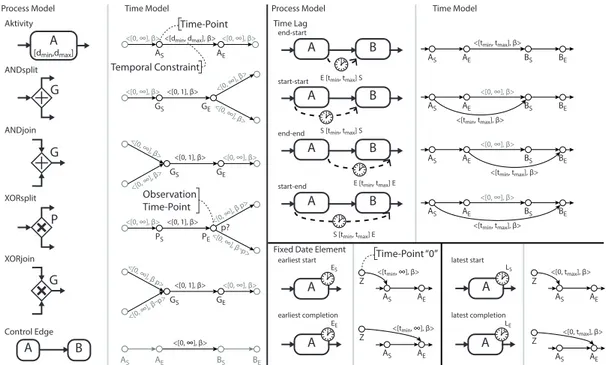
We denote the CSTN corresponding to a time-aware process model as its time model. The required mapping can roughly be described as follows:4 First, the control flow of the process model is mapped to a CSTN as illustrated in the left part of Figure 3. Particularly, each control flow element implicitly represents a temporal constraint, e.g., a control edge is equivalent to anE[0,∞]S time lag (cf. Figure 3). Each activity, ANDsplit, ANDjoin, and XORjoinni is represented as a pair of time-pointsNiS andNiE, corresponding to the starting and ending instant of the respective node (cf. Figure 3). In turn, for an XORsplit, the ending instant (i.e., NiE) is represented by an observation time-point (cf. Figure 3). Next, a constraint h[dmin, dmax]NiSNiE, iis added betweenNiSandNiE representing the duration [dmin, dmax] of the respective node.
Furthermore, for any control edge between nodesni andnj, a constrainth[0,∞]NiENjS, iis added between the time-points representing the ending instant ofni and starting instant ofnj (cf. Figure 3). If the source of the control edge corresponds to an XORsplit, in addition, the label of the constraint is augmented by propositionp=O−1(P). The latter represents the decision made at the corresponding observation time-point P, i.e., the label of the constraint h[0,∞]NiENjS, βibelonging to the “true”-branch is set to βp and the label of the “false”-branch toβ¬p(cf. Figure 3).5 Further, the labels of all constraints and time-points corresponding to activities, connectors and control edges in the XOR-block are augmented by eitherpor¬p depending on the branch they belong to.
Next, temporal constraints are mapped to the CSTN as depicted in the right part of Figure 3. A time laghISi[tmin, tmax]hITicorresponds to a constrainth[tmin, tmax]NihISiNjhITi,L(NihISi)∧L(NjhITi)ibetween the two time-points representing the respective instants of nodesni and nj (cf. Figure 3). In turn, a fixed date element is initially represented as a constrainth[0,∞]ZNhDi,L(NhDi)iwithZ being a special time-point representing time “0” (cf. Figure 3). During run-time, value [0,∞] of the constraint will be updated according to the actual fixed date chosen. Finally, process duration [dmin, dmax] is represented as constrainth[dmin, dmax]N0SNkE, i between the time-points representing the starting instant N0S of the first and the one representing the ending instantNkE of the last node of the process.
As example re-consider Figure 2. In particular, note that the labels of the constraints representing the XOR-block are either set topor¬p. Further, note that for the sake of readability, all edges without annotation are assumed to have boundsh[0,∞], i.
Based on Definition 2, we formally define the notion of temporal consistency for time-aware process models.
Definition 3(Temporal Consistency). A CSTNhT,C, L,OT,O, Piis called weakly consistent iff for each scenariosP at least one viable solution exists [8].
A time-aware process model is denoted as temporally consistent iff the corresponding time model (i.e., its CSTN representation) is weakly consistent.
When executing a time-aware process model, temporal consistency of the respective instances needs to be continuously monitored and re-checked. For this purpose, theminimal network of a CSTN6 must be determined.
4For further details we refer to [4], where we show how time-aware processes can be transformed to CSTNU—a special kind of CSTN.
5Note that this can be easily extended to consider more than two branches, but for the sake of simplicity, we only consider two branches in this paper.
6The minimal network of a CSTN is also called itsdispatchable form.
Time Model
<[dmin, dmax], β>
AS AE
<[0, ∞], β> <[0, ∞], β> <[tmin, tmax], β>
AE
AS BS BE
<[0, 1], β>
GS GE
<[0, ∞], β>
<[0,
∞], β>
<[0, ∞], β>
<[0, 1], β>
PS PE
<[0, ∞], β>
<[0,
∞], β¬p>
<[0, ∞], β p>
p?
<[0, 1], β>
GS GE
<[0, ∞], β>
<[0,
∞], β>
<[0, ∞], β>
<[0, 1], β>
GS GE
<[0, ∞], β>
<[0,
∞], β p>
<[0, ∞], β¬p>
Time Model Aktivity
<[0, ∞], β>
AE
AS BS BE
Control Edge
Time Lag
Fixed Date Element ANDsplit
ANDjoin
XORsplit
XORjoin
A B
E [tmin, tmax] S
<[tmin, tmax], β>
AE
AS BS BE
<[0, ∞], β>
A B
S [tmin, tmax] S
AE
AS BS BE
<[tmin, tmax], β>
<[0, ∞], β>
A B
E [tmin, tmax] E
AE
AS BS BE
<[tmin, tmax], β>
<[0, ∞], β>
A B
S [tmin, tmax] E end-start
start-start
end-end
start-end
earliest start latest start
earliest completion latest completion
A
EE
A
LE
A
ES
A
LS
AE
AS
Z <[tmin, ∞], β>
AE AS Z <[tmin, ∞], β>
AE
AS
Z <[0, tmax], β>
AE
AS
Z <[0, tmax], β>
[dminA,dmax]
A B
Process Model Process Model
G
G
G P
Time-Point
Time-Point “0”
Observation Time-Point Temporal Constraint
Figure 3: Process Modeling Elements and their Mapping to CSTN
Definition 4(Minimal Network). The minimal networkof a CSTNS=hT,C, L,OT,O, Piis the unique CSTN M = hT,C0, L,OT,O, Pi having the same set of solutions as S and each value allowed by any constraintc = h[x, y]XY, βi ∈ C0 being part of at least one solution of S for every scenario sP for which sP(β) =true.
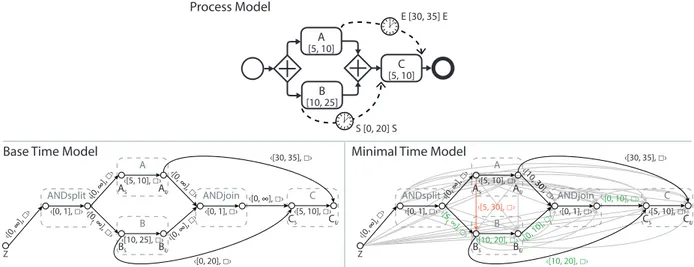
For any CSTN S a minimal network exists iff S is weakly consistent. In particular, such a minimal network provides a restricted set of constraints: As long as the value of each time-point is consistent with all constraints referring to it whose labels are still satisfiable, we can guarantee that the entire CSTN is weakly consistent. Besidesexplicit constraintsc∈ C we obtain when mapping the process model to the CSTN, the minimal network containsimplicit constraints between any pair of time-points that may occur in the same execution path. Note that these implicit constraints represent the effects the explicit constraints have on the overall CSTN (i.e., they represent interdependencies between explicit constraints). The implicit constraints are derived from the explicit ones when determining the minimal network. How to determine the latter is described in [8]. In the following, we denote the time model resulting from the mapping of the process model to a CSTN asbase time model and its minimal network asminimal time model of the process model.
As example consider Figure 4 which depicts a process model, its base time model and the corresponding minimal time model. Note that for the sake of readability most implicit constraints of the minimal time model are only indicated through light grey arrows. Further note, that explicit constraints which are restricted when minimizing the time model are highlighted in green. The example also illustrates some of the possible interdependencies between the various temporal constraints of a process model. In particular, the time lag between the start of activityBand start of Crestricts the maximum duration of Bto 20; note the constraint betweenBS andBE in the minimal time model. Moreover, the time lags betweenAandC andBandCintroduces an additional interdependency between activitiesAandB(the respective implicit temporal constraint is highlighted in red in Figure 4). In particular, although activitiesAandBare seemingly temporally unrelated,Bmay be started the earliest 5 time units after the start ofA. Otherwise, some temporal constraints of the process model cannot be satisfied. As a consequence,Bmay be started the earliest 5 time units after completion of the ANDsplit node. Furthermore,Bmust be started the latest 30 time units after the start of A. Note that representing all these interdependencies of different temporal constraints as part of the process model is not feasible as they can be quite numerous. Particularly, this would render the process model unreadable.
‹[10, 25], □›
‹[0, 1], □› ‹[0, 1], □› ‹[5, 10], □›
‹[30, 35], □›
‹[0, 20], □›
‹[0, ∞], □›
‹[0, ∞], □›
‹[0, ∞], □›
‹[0, ∞], □›
‹[0,
∞], □›
‹[0,
∞], □›
‹[5, 10], □›
BS BE
CS CE
AS AE
Z
ANDsplit ANDjoin C
A
B
Base Time Model
‹[10, 20], □›
‹[5, 30], □›
‹[0, 1], □› ‹[0, 1], □› ‹[5, 10], □›
‹[30, 35], □›
‹[10, 20], □›
‹[0, ∞], □›
‹[0, ∞], □›
‹[0, 10], □›
‹[0, 10], □›
‹[5,
∞], □›
‹[10, 30], □›
‹[5, 10], □›
BS BE
CS CE
AS AE
Z
ANDsplit ANDjoin C
A
B
Minimal Time Model A
B
C E [30, 35] E
S [0, 20] S [5, 10]
[10, 25]
[5, 10]
Process Model
Figure 4: Basic and Minimal Time Model
When executing a process instance, the two time models created at design-time are cloned. These clones are then kept up-to-date with the actual temporal state of the process instance (e.g., activity start and completion times) and used to monitor and re-check temporal consistency of the process instance [4].
4. Change Operations for Time-aware Processes
Standard change patterns adapting process models without temporal constraints have been extensively studied in literature [5]. This section discusses how respective change operations may be transferred to time- aware processes. Section 4.1 presents the change operations applicable to time-aware processes. Section 4.2 then provides an in-depth discussion of these change operations and shows how they can be extended to ensure temporal consistency of a changed process model.
4.1. Basic Change Operations
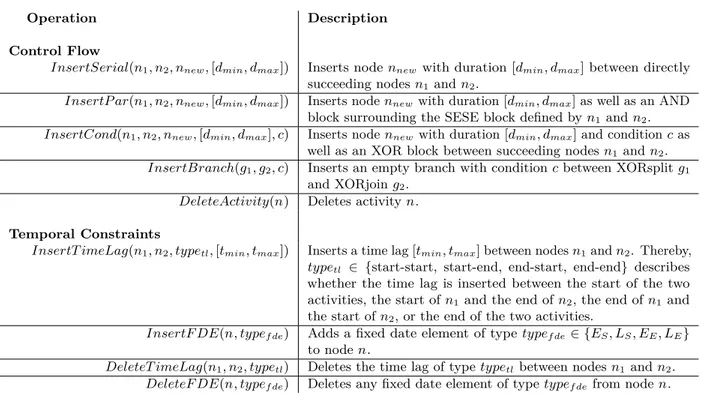
When changing a process schema or process instance, respectively, or—more generally—when changing a process model, the soundness of the latter must be ensured. To achieve this, our framework abstracts from low-levelchange primitives(e.g., adding an edge or node) to higher-levelchange operationswith well-defined pre-/post-conditions [5]. When being applied to a sound process model, such a high-level change operation (e.g., inserting a node in serial between two succeeding nodes) guarantees that the resulting process model will be structurally and behaviourally sound as well [5]. The upper part of Table 2 gives an overview of the most important change operations required for structurally modifying a process model. Note that these change operations may be combined to realize more complex change patterns [14] (e.g., move activity). We extend the set of structural change operations by a new set of change operations enabling us to modify the temporal constraints of a process model as well, e.g., inserting a time lag (see the bottom of Table 2).
Altogether, these change operations allow changing a time-aware process model, while guaranteeing structural and behavioural soundness of the resulting process model.
4.2. Applying Change Operations to Time-aware Processes
When modifying the model of a time-aware process, it must be ensured that the resulting process model is temporally consistent. This section defines basic criteria ensuring that the application of a change operation does not result in a temporally inconsistent process model. We further analyze the local impact a particular change operation has on the temporal properties of the respective process model, i.e., its temporal constraints.
If a change operation is applied to a process instance, additional state-specific pre- and post-conditions need to be met [5]. These are not considered in the following since they apply to time-aware processes as well. Further, note that any time-related instance-specific information is captured in the corresponding time
Operation Description Control Flow
InsertSerial(n1, n2, nnew,[dmin, dmax]) Inserts nodennew with duration [dmin, dmax] between directly succeeding nodesn1 andn2.
InsertP ar(n1, n2, nnew,[dmin, dmax]) Inserts nodennewwith duration [dmin, dmax] as well as an AND block surrounding the SESE block defined byn1 andn2. InsertCond(n1, n2, nnew,[dmin, dmax], c) Inserts nodennew with duration [dmin, dmax] and conditioncas
well as an XOR block between succeeding nodesn1andn2. InsertBranch(g1, g2, c) Inserts an empty branch with conditioncbetween XORsplitg1
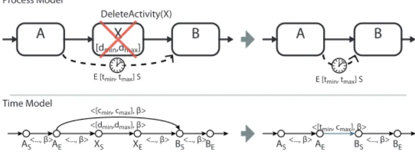
and XORjoing2. DeleteActivity(n) Deletes activityn. Temporal Constraints
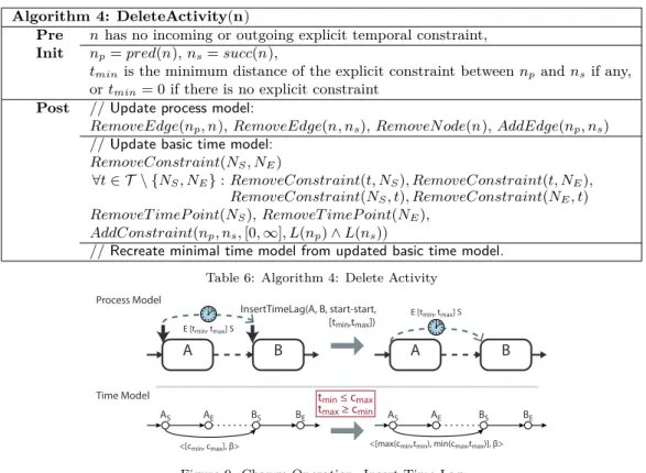
InsertT imeLag(n1, n2, typetl,[tmin, tmax]) Inserts a time lag [tmin, tmax] between nodesn1andn2. Thereby, typetl ∈ {start-start, start-end, end-start, end-end} describes whether the time lag is inserted between the start of the two activities, the start ofn1 and the end ofn2, the end ofn1and the start ofn2, or the end of the two activities.
InsertF DE(n, typef de) Adds a fixed date element of typetypef de ∈ {ES, LS, EE, LE} to noden.
DeleteT imeLag(n1, n2, typetl) Deletes the time lag of typetypetlbetween nodesn1 andn2. DeleteF DE(n, typef de) Deletes any fixed date element of typetypef de from noden.
Table 2: Basic Change Operations
model (cf. Section 3.2). In particular, we will show that it is sufficient to only consider the current minimal time model of the process instance.
4.2.1. Serial Activity Insertion.
As first change operation we considerInsertSerial(n1, n2, nnew,[dmin, dmax]). It allows inserting a node nnewwith duration [dmin, dmax] between two directly succeeding nodesn1 andn2 (cf. Figure 5). In terms of change primitives, this can be realized by deleting the control edge between nodesn1 andn2, followed by adding nodennew with duration [dmin, dmax] to the process model and properly connecting it ton1and n2by adding two new control edges (cf. Figure 5 and Table 3). Regarding the temporal properties of the resulting process model, one can observe that the insertion of nnew will first and foremost increase the minimum time distance betweenn1 andn2 todmin. By contrast, the maximum distance between the two nodes is not affected by the change as the newly added control connectors do not constrain it. Accordingly, if for the minimal time model the minimum durationdmin is compliant with any implicit or explicit constraint h[cmin, cmax]N1EN2S, βibetween the ending instant ofn1 and the starting instant ofn2 (i.e.,dmin≤cmax), the node insertion will not affect temporal consistency of the process model.7 Remember that each value of each constraint in the minimal time model is part of at least one solution (cf. Definition 4), i.e., one viable execution of the process model. Consequently, the time-aware process model is still temporally consistent.
After inserting the node into the process model, the mapping of this node and the control edges must be added to the time models as well (i.e., the base time model and minimal time model). Furthermore, the minimal time model must be locally adapted in order to properly cover the changes. In particular, the constraint between the ending instant ofn1 and the starting instant ofn2must be updated to [max{cmin, dmin}, cmax] to consider the new minimum distance between the two nodes (cf. Figure 5), i.e., certain values permitted by the old constraint might no longer be part of any viable solution. It further becomes evident that the constraints corresponding to the two control edges must be initialized to [0, cmax−dmin] (cf. Figure 5).
Algorithm 1 defines the pre- and post-conditions for applying change operationInsertSerial to a process model.
7Note that any implicit constraint h[cmin, cmax]N1EN2S, βi is always at least as restrictive as any explicit time lag E[tmin, tmax]Sbetweenn1 andn2.
<[max{cmin,dmin}, cmax], β>
<[dmin,dmax], β>
<[0, cmax-dmin], β> <[0, cmax-dmin], β>
AS<..., β>AE XS XE BS<..., β>BE
<[cmin, cmax], β>
<..., β> <..., β>
AS AE BS BE
dmin ≤ tmax
A X
[dmin,dmax] B A
[dminX,dmax]
B
E [tmin, tmax] S E [tmin, tmax] S
A
[dminX,dmax]
B
InsertSerial(A, B, X, [dmin,dmax])
E [tmin, tmax] S Process Model
Time Model
Figure 5: Change Operation: Insert Serial Algorithm 1: InsertSerial(n1,n2,nnew,[dmin,dmax])
Pre succ(n1) =n2,
∀h[cmin, cmax]N1EN2S, βi ∈ C:cmax≥dmin
Init γ=L(N1E)∧L(N2S) Post // Update process model:
RemoveEdge(n1, n2),
AddN ode(nnew,[dmin, dmax], Activity),AddEdge(n1, nnew),AddEdge(nnew, n2) // Update basic and minimal time model:
AddT imeP oint(NnewS, γ),AddT imeP oint(NnewE, γ), AddConstraint(NnewS, NnewE,[dmin, dmax], γ),
AddConstraint(N1E, NnewS,[0,∞], γ),AddConstraint(NnewE, N2S,[0,∞], γ), // Adapt minimal time model:
∀h[cmin, cmax]N1EN2S, βi ∈ C:
AddConstraint(N1E, NnewS,[0, cmax−dmin], β), AddConstraint(NnewE, N2S,[0, cmax−dmin], β),
U pdateConstraint(N1E, N2S,[max{cmin, dmin}, cmax)], β) Table 3: Algorithm 1: InsertSerial
After adding the node to the process model, the mapping of this node and the control edges must be added to the time models as well (i.e., the base time model and minimal time model). Further, the minimal time model must be locally adapted to properly cover the changes. In particular, the constraint between the ending instant ofn1 and the starting instant ofn2 must be updated to [max{cmin, dmin}, cmax] in order to consider the new minimum distance between the two nodes (cf. Figure 5), i.e., certain values permitted by the old constraint might no longer be part of any viable solution. It further becomes evident that the constraints corresponding to the two control edges must be initialized to [0, cmax−dmin] (cf. Figure 5).
Algorithm 1 defines the pre- and post-conditions for applying change operationInsertSerial to a process model.
After applyingInsertSerialthe changes made to the minimal time model need to be propagated to all other constraints to remove values no longer contributing to any solution. Note that this must be accomplished before performing any other change or resuming the execution of the process instance. Practically, this means that the minimality of the changed minimal time model needs to be restored. This may be achieved by applying the same algorithm initially used for determining the minimal time model (cf. Section 3.2).
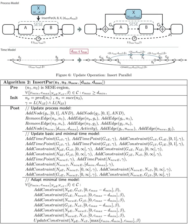
4.2.2. Parallel Activity Insertion.
The next change operation considered by us is operationInsertPar(n1, n2, nnew,[dmin, dmax]). It inserts nodennew together with an ANDsplit- and ANDjoin-gateway surrounding the SESE-region defined byn1 andn2(cf. Figure 6 and Table 4). This is achieved by serially inserting ANDsplit gsbetweenn1 and its predecessor and ANDjoingj betweenn2 and its successor (cf. InsertSerial-operation). Next, nodennew with duration [dmin, dmax] is added to the process model and properly connected to gsandgj by adding two new control edges (cf. Figure 6). Concerning temporal constraints, we again observe that inserting the node solely increases the minimum time distance between the predecessornp of n1 and the successorns ofn2. Consequently, if the minimum durationdmin is compliant with any implicit (or explicit) constrainth[cmin,
<[dmin,dmax], β>
XS XE
<[max{cmin,dmin},cmax], β>
AS
GsS GsE GjS GjE
BE
<[0, cmax-dmin], β> <[0, cmax-dmin], β>
<[cmin, cmax], β>
AS BE
dmin ≤ tmax
[dminX,dmax]
E [tmin, tmax] S
A SESE B
Gs Gj
[dminX,dmax]
InsertPar(A, B, X, [dmin,dmax])
A SESE B
E [tmin, tmax] S Process Model
Time Model
Figure 6: Update Operation: Insert Parallel Algorithm 2: InsertPar(n1,n2,nnew,[dmin,dmax])
Pre (n1, n2) is SESE-region,
∀h[cmin, cmax]NpENsS, βi ∈ C:cmax≥dmin, Init np=pred(n1) ,ns=succ(n2),
γ=L(N1E)∧L(N2S) Post // Update process model:
AddN ode(gs,[0,1], AN D),AddN ode(gj,[0,1], AN D), RemoveEdge(np, n1),AddEdge(np, gs),AddEdge(gs, n1), RemoveEdge(n2, ns),AddEdge(n2, gj),AddEdge(gj, ns),
AddN ode(nnew,[dmin, dmax], Activity),AddEdge(gs, nnew),AddEdge(nnew, gj), // Update basic and minimal time model:
AddT imeP oint(GsS, γ),AddT imeP oint(GsE, γ),AddConstraint(GsS, GsE,[0,1], γ), AddT imeP oint(GjS, γ),AddT imeP oint(GjE, γ),AddConstraint(GjS, GjE,[0,1], γ), AddConstraint(NpE, GsS,[0,∞], γ),AddConstraint(GsE, N1E,[0,∞], γ),
AddConstraint(N2E, GjS,[0,∞], γ),AddConstraint(GjE, NsS,[0,∞], γ), AddT imeP oint(NnewS, γ),AddT imeP oint(NnewE, γ),
AddConstraint(NnewS, NnewE,[dmin, dmax], γ),
AddConstraint(NpE, NnewS,[0,∞], γ),AddConstraint(NnewE, NsS,[0,∞], γ), AddConstraint(GsE, NnewS,[0,∞], γ),AddConstraint(NnewE, GjS,[0,∞], γ) // Adapt minimal time model:
∀h[cmin, cmax]NpENsS, βi ∈ C:
AddConstraint(NpE, GsS,[0, cmax−dmin], β), AddConstraint(GsE, NnewS,[0, cmax−dmin], β), AddConstraint(NnewE, GjS,[0, cmax−dmin], β), AddConstraint(GjE, NsS,[0, cmax−dmin], β), AddConstraint(NpE, NnewS,[0, cmax−dmin], β), AddConstraint(NnewE, NsS,[0, cmax−dmin], β), U pdateConstraint(NpE, NsS,[max{cmin, dmin}, cmax], β)
Table 4: Algorithm 2: InsertPar
cmax]NpENsS, βi between the respective instants ofnp andns, performing the change operation does not impact consistency of the process model. Note that the added ANDsplit and ANDjoin gateways constitute silent nodes.
Again, after structurally modifying the process model, the time models needs to be adapted to reflect the change. Particularly, in the minimal time model the temporal constraint between the ending instant ofnp
and the starting instant ofnsmust be updated to [max{cmin, dmin}, cmax] (cf. Figure 6). Moreover, the constraints representing the newly added control edges must be initialized to [0, cmax−dmin] to reflect the impact the other constraint have on the time to executed the new activity (cf. Figure 6). Algorithm 2 (cf.
Table 4) formally defines these pre- and post-conditions for performing operationInsertPar.
At last, the changes made to the minimal time model need to be propagated to the other constraints
![Figure 5: Change Operation: Insert Serial Algorithm 1: InsertSerial(n 1 , n 2 , n new , [d min , d max ])](https://thumb-eu.123doks.com/thumbv2/1library_info/5213371.1669066/10.892.144.744.161.627/figure-change-operation-insert-serial-algorithm-insertserial-new.webp)