Marine mineral exploration with controlled-source
1
electromagnetics at the TAG hydrothermal field, 26
◦N
2
Mid-Atlantic Ridge
3
R. A. S. Gehrmann1, L. A. North2, S. Graber3, F. Szitkar4, S. Petersen3, T.
4
A. Minshull1and B. J. Murton2
5
1University of Southampton, Ocean and Earth Sciences, National Oceanography Centre Southampton,
6
UK
7
2National Oceanography Centre, Natural Environment Research Council, Southampton, UK
8
3GEOMAR, Helmholtz Centre for Ocean Research Kiel, Germany
9
4Japan Agency for Marine-Earth Science Technology, JAMSTEC, Centre for Earthquakes and Tsunami,
10
Japan
11
Key Points:
12
• Seafloor massive sulphide deposits can be detected/mapped on a large scale with
13
controlled source electromagnetic methods.
14
• Multidisciplinary geophysical data analysis and local probing lead to a rigorous
15
interpretation of deposit dimensions and resource potential.
16
• Sulphide ore content reduces with depth down to a few tens of meters into the de-
17
posit’s altered basalt and silica-dominated root.
18
Corresponding author: Romina Gehrmann,r.a.gehrmann@soton.ac.uk
This article has been accepted for publication and undergone full peer review but has not been through the copyediting, typesetting, pagination and proofreading process which may lead to differences between this version and the Version of Record. Please cite this article as doi:
10.1029/2019GL082928
Abstract
19
Seafloor massive sulphide (SMS) deposits are of increasing economic interest in order to
20
satisfy the relentless growth in worldwide metal demand. The Trans-Atlantic Geotra-
21
verse (TAG) hydrothermal field at 26◦N on the Mid-Atlantic Ridge hosts several such
22
deposits. This study presents new controlled source electromagnetic (CSEM), bathymet-
23
ric and magnetic results from the TAG field. Potential SMS targets were selected based
24
on their surface expressions in high-resolution bathymetric data. High-resolution reduced-
25
to-the-pole magnetic data show negative anomalies beneath and surrounding the SMS
26
deposits, revealing large areas of hydrothermal alteration. CSEM data, sensitive to the
27
electrical conductivity of SMS mineralization, further reveal a maximum thickness of up
28
to 80 m and conductivities of up to 5 S/m. SMS samples have conductivities of up to
29
a few thousand S/m, suggesting that remotely inferred conductivities represent an av-
30
erage of metal sulphide ores combined with silicified and altered host basalt that likely
31
dominates at greater depths.
32
Plain language summary
33
Seafloor massive sulphide deposits, formed by high-temperature hydrothermal activity,
34
provide a potential resource for metals including copper, zinc, lead, gold, and silver. Here,
35
we report the results of a geophysical study to estimate the distribution and size of seafloor
36
ore deposits at the Trans-Atlantic Geotraverse (TAG) hydrothermal field, located south
37
of the Azores, on the Mid-Atlantic Ridge (MAR). The TAG field hosts numerous deposits,
38
all but one of which are hydrothermally inactive. Inactive deposits are economically more
39
valuable but difficult to detect. Our solution is a combination of high-resolution seafloor
40
and sub-seafloor mapping techniques. By focusing on exploration using ship-towed elec-
41
tromagnetic sensing and autonomous underwater vehicle-based mapping and character-
42
isation of their magnetic field, we exploit unique signatures identifying these deposits from
43
their surrounding volcanic rock. These data enable us to delineate the extent of the de-
44
posits and provide a first estimate of their thickness. We integrate physical and chem-
45
ical properties of ore and host rock samples, recovered by drilling, into our interpreta-
46
tion in order to estimate the full economic potential of the deposits. Our results reveal
47
a deposit geometry consisting of a sulphide ore body that is mixed with an increasing
48
amount of silica and altered volcanic rocks at depth.
49
1 Introduction
50
Seafloor massive sulphide (SMS) deposits are considered a potential resource for
51
economically valuable metals such as copper, zinc, lead, gold, silver as well as for trace
52
metals necessary for green or new technologies. Increasing global demand and insecure
53
supply on land lead many countries to target the deep sea for future mineral resources
54
(Hannington, Jamieson, Monecke, Petersen, & Beaulieu, 2011; Rona, 2003). While ac-
55
tive vent fields are dominantly explored using geochemical sensors that search for anoma-
56
lies in the water column, inactive fields do not exhibit such a prominent signature. In-
57
active SMS deposits, however, are estimated to contain a larger amount of metal sulphides,
58
and are characterized by the absence of high-temperature venting and the commonly as-
59
sociated low pH-values: two factors viewed as positive for possible mining operations (Han-
60
nington et al., 2011). The assessment of the quality and amount of SMS deposits suf-
61
ficient for resource calculations requires both fast and cost-effective remote exploration
62
to evaluate the distribution and size of the deposits, and localised drilling to understand
63
the resource potential of any given site.
64
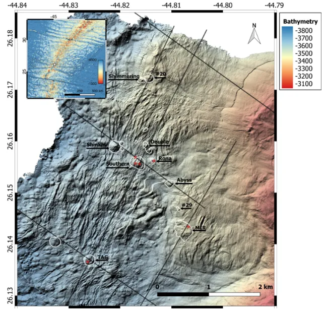
The Trans-Atlantic Geotraverse (TAG) field (Figure 1), located at 26◦08’N, cov-
65
ering an area of about 5x5 km2 is the largest and best studied hydrothermal field on the
66
Mid-Atlantic Ridge (MAR). It hosts, in addition to the active TAG mound, several in-
67
active SMS deposits. Hydrothermal activity in the area may have started as early as 140 kyr
68
ago (Humphris et al., 1995). Radiometric data indicated that the formation of massive
69
sulphides at the active TAG mound started some 50 to 20 kyr ago with high-temperature
70
pulses every 5-6 kyr (Lalou, Reyss, Brichet, Rona, & Thompson, 1995). The inactive sul-
71
phide occurrences comprise the MIR zone, the oldest deposit, to the east of TAG mound,
72
and a number of mounds to the north of TAG mound in an area that was originally called
73
the Alvin zone (Rona et al., 1993). The Alvin zone includes the large Shinkai, South-
74
ern, Shimmering and Double Mound (White, Humphris, & Kleinrock, 1998) as well as
75
a series of smaller sulphide mounds (e.g., Rona Mound, Figure 1).
76
During summer 2016 an international and interdisciplinary survey with two back-
77
to-back cruises was conducted in the TAG hydrothermal field to study the geophysical
78
and geochemical signature of SMS deposits. The survey comprised high-resolution bathy-
79
metric mapping, and magnetic data acquisition from the autonomous underwater vehi-
80
cle (AUV) Abyss (GEOMAR), and controlled source electromagnetic (CSEM) experi-
81
ments among others. Additionally, seafloor coring with the lander-type seafloor drilling
82
rig RD2 (British Geological Survey), and video imaging with the remotely operated ve-
83
hicle (ROV) HyBis (National Oceanography Centre) were also conducted. Physical and
84
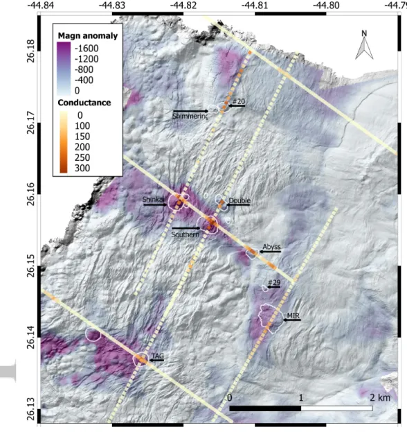
chemical properties of the sulphide samples and sediment cores were measured shore-
85
side in the lab (Murton et al., 2019). Here, we present results from this work with em-
86
phasis on the towed CSEM study regarding SMS detection and size estimation.
87
The CSEM method is sensitive to contrasts in electrical conductivity. For exam-
88
ple, the largest component of an SMS deposits is expected to be precipitated sulphide
89
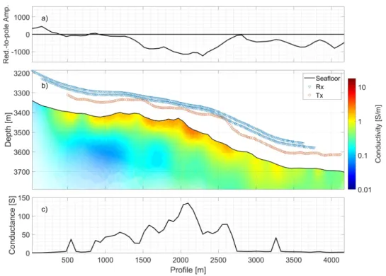
(e.g., pyrite, iron sulphide) which is a semiconductor. According to drilling results ob-
90
tained by the Ocean Drilling Program on TAG mound (Herzig, Humphris, Miller, & Zieren-
91
berg, 1998; Humphris et al., 1995) and RD2 drilling on the inactive mounds (Lehrmann,
92
Stobbs, Lusty, & Murton, 2018), the host rock underneath the deposits is likely to com-
93
prise less conductive fresh and hydrothermally altered basalts for which conductivity is
94
controlled by electrolytes (salt water) in the pore space. Due to the mound size (up to
95
a few hundreds of meters in diameter) and their potential for significant conductivity con-
96
trasts, SMS deposits may be detected with remote electromagnetic methods such as hor-
97
izontal dipole-dipole arrays (Cairns, Evans, & Edwards, 1996; Edwards & Chave, 1986;
98
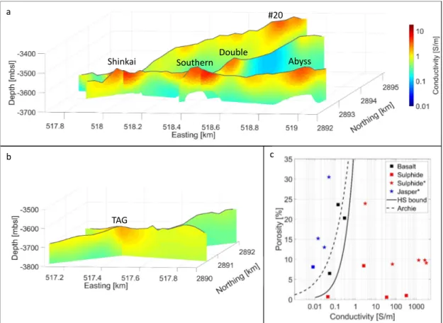
Evans & Everett, 1994). Here, we present new CSEM data acquired over several kilo-
99
meters with a large footprint of up to a few hundred meters interpreted with comple-
100
mentary interdisciplinary data to solve the problem of reliable resource assessment for
101
SMS deposits.
102
2 Methods
103
2.1 Controlled Source Electromagnetics
104
The CSEM system presented here is comprised of the Deep-towed Active Source
105
Instrument (DASI, Sinha, Patel, Unsworth, Owen, & MacCormack, 1990) and two three-
106
axis electric field receivers (Vulcan, Constable, Kannberg, & Weitemeyer, 2016) towed
107
at 350 m and 505 m behind DASI. The DASI-Vulcan array was towed between 50 to 150 m
108
above the seafloor at a constant speed of 1 kn. An alternating square waveform with a
109
current amplitude of about 90 A, and a base frequency of 1 Hz was transmitted through
110
a 50-m long bipole antenna. Six multi-kilometer-long survey profiles were acquired across
111
the active TAG mound and several inactive SMS deposits (Figure 1).
112
Data processing comprised a fast-Fourier transformation of 1-s long time windows,
113
deconvolution with the transmitter signal and stacking of 30-s long windows (Text S1,
114
Myer, Constable, & Key, 2011). Including navigational information, the amplitude of
115
the data for frequencies of 1 – 5 Hz were evaluated along each profile. There is no di-
116
rect way to interpret CSEM data for a heterogeneous seafloor conductivity model. In-
117
stead, the conductivity model below the seafloor must be inferred with inversion algo-
118
rithms. Here, we implement a two-dimensional (2D) inversion (MARE2DEM, Key, 2016):
119
a linearised scheme based on Occam’s razor, searching for the simplest model that can
120
explain the data (Text S1, Constable, Parker, & Constable, 1987). The final conductiv-
121
ity model favours gradual changes, and only includes abrupt changes between model cells
122
if the data sensitivity is high enough. Generally, data sensitivity reduces with increas-
123
ing depth but also depends on the assumed data error, which we have assessed with a
124
detailed error analysis using forward modelling that includes uncertainties caused by nav-
125
igation over rough terrain (Text S1). Also, an ambiguity arises between a thicker, less
126
conductive body and a thinner, more conductive body. In fact, the conductivity-thickness
127
product, the conductance, can often be better resolved (e.g., Edwards, 1997) than in-
128
dividual parameters alone. Despite this ambiguity, the inferred thickness does not de-
129
viate by more than a few tens of meters from the actual thickness because the model is
130
constrained by two receivers at different offsets to the source and three different frequen-
131
cies, allowing the dipole-dipole system to be sensitive to the less conductive material be-
132
low the sulphide ore body.
133
For each profile, the conductance is calculated as the integrated conductivity-thickness
134
product for 5 m intervals from the seafloor down to the the depth where conductivity
135
decreases to 1 S/m. We relate conductivities greater than 1 S/m to increasing amounts
136
of conductive metal sulphides mixed with less conductive seawater-saturated fresh and
137
altered basalts.
138
2.2 Bathymetry
139
The TAG hydrothermal field has been mapped with high-resolution (2 m, Figure 1)
140
bathymetric surveys using an AUV-based multibeam echosounder. The SMS mounds have
141
an almost circular base and a smooth to steep/rugged slope and confirm previous ob-
142
servations on lower resolution data (White et al., 1998). Examples of these mounds are
143
Shinkai, Southern and Double Mound (Figure 1) which are of conical shape. The MIR
144
zone on the other hand has a more complex relief and a larger diameter. Inactive SMS
145
mounds can be easily mistaken with volcanic mounds which consist mainly of basalt, al-
146
though the latter have a more regular shape and have lower slope angles as is also the
147
case at Endeavour Ridge (Jamieson, Clague, & Hannington, 2014) .
148
2.3 Magnetics
149
The magnetic signature of the hydrothermal field (Szitkar & Dyment, 2015; Tivey,
150
Rona, & Kleinrock, 1996; Tivey, Rona, & Schouten, 1993) reveals a lack of magnetiza-
151
tion below the active and inactive mounds which is likely caused either by alteration of
152
the magnetic minerals of the upper crust during hydrothermal circulation and/or by the
153
volume filled with non-magnetic SMS deposits between the magnetometer and the oceanic
154
crust (Szitkar, Petersen, Caratori Tontini, & Cocchi, 2015). The magnetic data were recorded
155
with the triaxial flux-gate sensor mounted on the AUV while flown at different altitudes
156
between 20 and 100 m above the seafloor. Raw data were then adjusted for the effect
157
of the vehicle magnetic signature, low-pass filtered and interpolated on a grid. Finally,
158
magnetic anomalies were reduced-to-the-pole using the local inclination and declination
159
of the geomagnetic field to place them above their causative sources within the crust.
160
2.4 Rock Physics
161
Rock samples were collected from TAG (SMS and Jasper samples) either at out-
162
crops on the seafloor by ROV HyBis or during sub-seafloor drilling (RD2, Lehrmann
163
et al., 2018). These were supplemented by reference samples from outcrops on land (e.g.,
164
basalt from Cyprus). Samples where the electrical conductivity mechanism is dominated
165
by ionic conduction in pore space (i.e., non-SMS samples) were measured with an ionic
166
conductivity cell based on the device described by Zisser and Nover (2009). Because this
167
configuration is susceptible to measurement artefacts caused by double layer polarisa-
168
tion at any semiconductor (such as metal sulphides) to electrolyte interface (Stojek, 2010),
169
the sulphide samples were measured using direct contact and/or inductive methods (Text
170
S2).
171
3 Results
172
Inferred conductances are elevated for all known inactive deposits in the MIR and
173
Alvin zone as well as the active TAG mound and coincide with negative reduced-to-the-
174
pole magnetic anomalies (Figure 2). The observed CSEM data are fit well by the mod-
175
els (Figure S2), but biases remain, that are likely due to systematic errors such as the
176
rough topography and the 3D characteristics of the SMS target given the large footprint
177
of the DASI-Vulcan array. A 2D inversion of data from a conical 3D structure may re-
178
sult in biases in the predicted vs. observed data and the inversion model may contain
179
artefacts below and next to the mound structure, but the elevated conductivity within
180
the mound can still be resolved adequately (Haroon et al., 2018).
181
3.1 MIR zone
182
The MIR zone is located 4 km east off the MAR axis and covers a large area (∼1 km
183
in diameter) with the only mound-like feature being<10 m high. Elevated heat-flow val-
184
ues (Rona et al., 1996) indicate a late stage of hydrothermal activity. From the inferred
185
final conductivity model for the North-South profile over the MIR zone (Figure 3b), a
186
50-m thick, elongate, conductive anomaly is present immediately beneath the seafloor.
187
The magnetic profile for the profile across the MIR zone (Figure 3a) is interpolated
188
from the reduced-to-the-pole magnetic map (Figure 2). A negative magnetic anomaly
189
encompasses the maximum of the conductance (Figure 3c) along the profile. For most
190
other SMS deposits, the highest conductances reside within the much larger areal extents
191
of the magnetic anomalies that often connect adjacent deposits.
192
Although the CSEM method is sensitive to resistivity contrasts at the base of the
193
sulphide deposit (Note: model cells with low data sensitivity are blanked out in Figure 3b),
194
a strong conductivity contrast is not typically resolved because the sulphide content likely
195
changes gradually with depth and because the inversion algorithm also favours smooth
196
transitions.
197
3.2 Alvin zone
198
The Alvin zone (Rona et al., 1993) encompasses the northern part of the hydrother-
199
mal field including Shinkai, Southern, Double, Rona and Shimmering Mound. Shinkai,
200
target #20, Southern, Double and the newly identified Abyss Mound all exhibit distinct
201
conductivity anomalies with conductivities up to 5 S/m (Figure 4a). The root of the mounds
202
is expected to extend much deeper but the denser silica-rich wall-rock breccia and chlo-
203
ritized basalts tend to have much lower conductivities than the SMS deposits (Morgan,
204
2012). Seismic imaging of Shinkai and Southern Mound also support a deep reaching root
205
(∼220 m) consisting roughly of massive sulphide on top (∼first 100 m) and a stockwork
206
of brecciated sulphide, silica and altered basalt underneath (Murton et al., 2019). The
207
SMS deposit at Southern mound is inferred to be up to 80 m thick based on the CSEM
208
data alone (Figure 4a) with an average conductivity of 3.7 S/m. A conductance of up
209
to 300 S could also be translated in a thinner deposit of, for example, 60 m with an av-
210
erage conductivity of 5 S/m. Structures smaller than a few tens of meters are at the limit
211
of resolution, so that a thin 10 m deposit of conductive material on top of the mound
212
would appear as a thicker but less conductive cone top (Haroon et al., 2018). Southern
213
mound has also been studied with the coincident-loop system MARTEMIS, which is more
214
downward looking and has a much smaller footprint than the towed CSEM system, and
215
is more sensitive to conductive deposits with a higher vertical resolution but with a max-
216
imum penetration depth of about 50 m (Haroon et al., 2018; H¨olz & Jegen, 2016). The
217
1D inversion results of the MARTEMIS data reveal higher conductivities up to 10 S/m
218
for the upper∼50 m below the mound’s surface. Combining these observations suggests
219
that the top of the deposit has a higher percentage of metal sulphides than the deeper
220
sections.
221
The newly identified Abyss Mound SMS occurrence was verified by video obser-
222
vations (Petersen et al., 2016), and the presence of metalliferous sediments supports a
223
past history of hydrothermal activity (Dutrieux et al., 2017). Geological and geochem-
224
ical ground-truthing therefore strengthens the interpretation based on bathymetry, CSEM
225
and magnetics. The area to the north of Shimmering Mound (Figure 1) still shows some
226
low-temperature hydrothermal activity (Rona et al., 1998) but was not sampled during
227
our survey. A strong magnetic low and elevated conductivities, however, indicate hydrother-
228
mal deposition around an unnamed mound (#7 in Humphris, Tivey, & Tivey, 2015). Tar-
229
get #20 next to Shimmering Mound also shows high conductivities seemingly belong-
230
ing to the same hydrothermal system.
231
3.3 Active TAG mound
232
The TAG Mound is the only active mound in the TAG hydrothermal field. The
233
negative magnetic anomaly extends west of TAG and coincides with other bathymetry-
234
inferred targets. TAG Mound has much lower inferred conductivities of up to 2 S/m than
235
the inactive SMS mounds (Figure 4b). The active mound is different to the inactive mounds
236
in three ways. The temperatures are distinctly higher (up to 360◦C) which could poten-
237
tially increase the conductivities of the sulphides and pore fluids. On the other hand,
238
it is anhydrite rich, which has a lower conductivity than sulphides, but dissolves at lower
239
temperatures and is hence not present in the inactive mounds. The third difference is
240
its smaller size (estimates of 2.7 million tonnes for TAG Mound (Hannington, Galley,
241
Herzig, & Petersen, 1998) compared to up to 6.3 million tonnes for Southern Mound (Mur-
242
ton et al., 2019)). CSEM experiments in the 1990s at the TAG active mound with smaller
243
transmitter-receiver spacings (<100 m) showed average conductivities (for homogeneous
244
seafloor) of up to 16 S/m (Cairns et al., 1996), similar to the conductivities for a sim-
245
ilar penetration depth of the MARTEMIS system at the inactive deposits (Haroon et
246
al., 2018), suggesting that the lower inferred conductivities with the DASI-Vulcan sys-
247
tem at the TAG mound are more likely caused by the target size compared to the transmitter-
248
receiver spacing. The DASI-Vulcan system averages over a larger footprint and depth,
249
and the adjacent altered basalt and increasing amount of silicate with depth likely im-
250
pacts the large-scale inferred conductivity compared to the short-offset, high-resolution
251
methods. In fact, the geometry of the DASI-Vulcan array was chosen for fast, continuously-
252
towed, data collection over several kilometers with a wide footprint to detect SMS de-
253
posits large enough to be of economic interest.
254
3.4 Rock Physics
255
Conductivity measurements in the laboratory were made on five SMS samples col-
256
lected on the seafloor by the ROV HyBis, or recovered as core drilled by RD2 (Figure 1).
257
The conductivities of SMS samples are up to five orders of magnitude higher than the
258
reference basalt samples from outcrops on Cyprus, and although they have lower porosi-
259
ties (Figure 4c), they have the electrical conduction behavior characteristic of semicon-
260
ductors/metals. By comparison, for the case of electrolytic conduction, the conductiv-
261
ity is directly related to the porosity of the sample (e.g., Archie’s Law, Archie, 1942).
262
This relationship does not hold for SMS deposits, which act as semiconductors causing
263
the conductivities to be orders of magnitude higher and display complex behavior due
264
to their frequency-dependent chargeability (Spagnoli et al., 2016; Spagnoli, Weymer, Je-
265
gen, Spangenberg, & Petersen, 2017). Samples from the Central Indian Ridge show sim-
266
ilar behavior with a clear frequency dependence, e.g., larger conductivities at higher fre-
267
quencies (M¨uller et al., 2018). Here, the conductivities for the pure SMS samples are about
268
three orders of magnitude larger than the conductivities inferred from the remote DASI-
269
Vulcan array suggesting that the SMS deposits are locally richer and can be found at
270
shallow depth below the surface but are likely mixed with silicates and altered basalts
271
at greater depth. The results inferred from the DASI-Vulcan array average over the mound
272
and cannot resolve features and structure at scales of less than a few tens of meters.
273
4 Discussion and Conclusions
274
We have presented how remote geophysical techniques have been successfully im-
275
plemented to detect and localize SMS deposits in the TAG hydrothermal field. The deep-
276
towed controlled source electromagnetic DASI-Vulcan experiment has been used to cover
277
several-kilometer long profiles with a lateral footprint of up to a few hundred meters across
278
potential targets, some of which have been verified geologically before by localized sam-
279
pling and video observations, while others were only recognized as potential targets from
280
their shape (multi-beam mapping). The CSEM data have confirmed known deposits and
281
revealed previously uncertain ones. The inferred deposit thickness of up to 80 m is a max-
282
imum value as the inversion favours low conductivity gradients. Although the CSEM sys-
283
tem is sensitive to the conductivity contrast between the pyrite-dominated SMS cap and
284
the silicate-dominated stockwork, the product of thickness and conductivity can often
285
be better resolved than individual parameters alone. Inferred conductivities reach up to
286
5 S/m, indicating the presence of semi-conductors. The inferred values, however, are gen-
287
erally orders of magnitude lower than the conductivities of lab samples composed of pyrite
288
with interconnected chalcopyrite. These lab samples were collected at the SMS deposits
289
themselves and can reach conductivities of up to a few thousand S/m. The remotely in-
290
ferred values are therefore average conductivities for volumes larger than a few hundreds
291
of cubic meters likely with decreased connectivity. Although the inferred conductivity
292
structure is limited in resolution of a few tens of meters, the conductivity anomalies are
293
generally localised to the deposit. In comparison, negative magnetic anomalies gener-
294
ally extend over larger areas than the deposit footprint because magnetic data are sen-
295
sitive to the nonmagnetic SMS deposit itself, and to the hydrothermally-demagnetized
296
stockwork and fault zones that surround and underlay the deposits at greater depth. High-
297
resolution magnetics is therefore an indicator for where hydrothermal circulation was ac-
298
tive on a larger scale. Sulphide deposits also have distinct surface expressions such as
299
conical mounds and rough small-scale topography which can be interpreted with high-
300
resolution bathymetry as long as the deposits are not overprinted with sedimentation
301
or lava flows (camouflaged among volcanic, hummocky, mounds). Each of the geophys-
302
ical methods alone provide a piece to the puzzle, that evaluated individually may lead
303
to ambiguous interpretations, but together lead to a robust interpretations of the SMS
304
potential.
305
In this work, we studied several inactive deposits up to∼4 km from the ridge axis
306
as well as the active TAG Mound. TAG Mound shows lower conductivities than seawa-
307
ter, but is also smaller than most of the inactive deposits. Previous studies with a seafloor
308
EM transmitter and receiver spacings of<100 m (Cairns et al., 1996) revealed higher
309
conductivities (up to∼16 S/m), similar to the conductivities for a similar penetration
310
depth of the MARTEMIS system at the inactive deposits (Haroon et al., 2018) which
311
suggests that the generally lower conductivities observed with the DASI-Vulcan system
312
at TAG are probably related to the deeper penetration depth due to the larger transmitter-
313
receiver spacing (350 and 505 m), and resulting averaging between highly conductive ma-
314
terial just beneath the seafloor and less conductive stockwork material at greater depth.
315
The smaller size of the TAG Mound compared to the inactive deposits may in this case
316
play a larger role than the possible effects of anhydrite (Lehrmann et al., 2018; Murton
317
et al., 2019) and hot fluids (∼360◦C) which are only present in the active system.
318
To estimate the economic value of each deposit, it is essential to quantify the sub-
319
seafloor geometry and probe the seafloor to understand the overall evolution of the de-
320
posit. Lander-type drilling shows that the content of valuable elements such as copper
321
and zinc likely decreases with depth due to element remobilizing during the waning phase
322
of hydrothermal activity (Lehrmann et al., 2018). The rich content of copper and zinc
323
in surface samples and metalliferous sediments (Dutrieux et al., 2017) therefore does not
324
represent the element concentration at depth. The elevated conductivities at greater depths
325
might be caused by a large concentration of pyrite, which has no economic value (Mur-
326
ton et al., 2019). The deposit maximum thickness from CSEM extending beneath the
327
base of the mounds on the seafloor supports the findings of Teagle and Alt (2004) that
328
basaltic crust becomes heavily altered to secondary minerals such as silicates and chlo-
329
rites with SMS inclusions.
330
We have shown that bathymetry, magnetic and CSEM surveys are sensitive to dif-
331
ferent physical aspects of the deposits and therefore complement each other with a high
332
success rate for detection and characterization of inactive deposits.
333
Acknowledgments
334
We would like to thank the European Commission for funding the Framework 7 project
335
Blue Mining (Grant Number 604500). We thank all cruise participants and crew from
336
M127 and JC138 for their support in data acquisition especially Ian Tan, Sebastian H¨olz,
337
Eric Attias, and Geomar’s AUV Abyss team. We thank Karen Weitemeyer and Steve
338
Constable for their advice. We thank Ben Ollington, McKinley Morton and Amir Ha-
339
roon for their work with the data set. We thank Kerry Key for the inversion code MARE2DEM
340
and supporting matlab scripts as well as David Myer for processing routines and discus-
341
sions. Tim Minshull was supported by a Wolfson Research Merit award. We thank Mar-
342
ion Jegen for internally reviewing the article and two anonymous reviewers for their help-
343
ful comments to improve the manuscript. Data are available from Gehrmann (2019); Gehrmann,
344
North, Lehrmann, and Murton (2019); Petersen (2019).
345
References
346
Archie, G. E. (1942). The Electrical Resistivity Log as an Aid in Determining Some
347
Reservoir Characteristics. Trans. Am. Inst. Min. Metall. Pet. Eng.,146, 54-
348
62.
349
Cairns, G. W., Evans, R. L., & Edwards, R. N. (1996). A time domain electromag-
350
netic survey of the TAG Hydrothermal Mound. Geophysical Research Letters,
351
23(23), 3455-3458. doi: 10.1029/96GL03233
352
Constable, S. C., Kannberg, P. K., & Weitemeyer, K. (2016). Vulcan: A deep-towed
353
CSEM receiver. Geochemistry, Geophysics, Geosystems,17(3), 1042–1064. doi:
354
10.1002/2015GC006174
355
Constable, S. C., Parker, R. L., & Constable, C. G. (1987). Occam’s inversion: A
356
practical algorithm for generating smooth models from electromagnetic sound-
357
ing data. Geophysics,52, 289-300.
358
Dutrieux, A., Lichtschlag, A., Murton, B. J., Petersen, S., Barriga, F., & Martins, S.
359
(2017). Metal mobilization in hydrothermal sediments. Paper presented at 49th
360
Underwater Mining Conference, Berlin, Germany.
361
Edwards, R. N. (1997). On the resource evaluation of marine gas hydrate deposits
362
using sea-floor transient electric dipole-dipole methods. Geophysics,62(1), 63-
363
74.
364
Edwards, R. N., & Chave, A. D. (1986). A transient electric dipole-dipole method
365
for mapping the conductivity of the sea floor. Geophysics,5(4), 984-987.
366
Evans, R. L., & Everett, M. E. (1994). Discrimination of hydrothermal mound struc-
367
tures using transient electromagnetic methods. Geophysical Research Letters,
368
21(6), 501-504. doi: 10.1029/94GL00418
369
Gehrmann, R. A. S. (2019). Controlled-source electromagnetic data from the TAG
370
hydrothermal field, 26N Mid-Atlantic Ridge.[data set]. PANGAEA. Retrieved
371
fromhttps://doi.pangaea.de/10.1594/PANGAEA.899073
372
Gehrmann, R. A. S., North, L. J., Lehrmann, B., & Murton, B. J. (2019). Rock
373
physic samples from TAG, Mid-Atlantic Ridge, and various onshore samples
374
[data set]. PANGAEA. Retrieved fromhttps://doi.pangaea.de/10.1594/
375
PANGAEA.899411
376
Hannington, M. D., Galley, A. G., Herzig, P. M., & Petersen, S. (1998). 28. Com-
377
parison of the TAG mound and stockwork complex with Cyprus-type mas-
378
sive sulfide deposits. InProceedings-ocean drilling program scientific results
379
(Vol. 158, pp. 389–415).
380
Hannington, M. D., Jamieson, J., Monecke, T., Petersen, S., & Beaulieu, S. (2011).
381
The abundance of seafloor massive sulfide deposits. Geology, 39(12), 1155–
382
1158. doi: 10.1130/G32468.1
383
Haroon, A., H¨olz, S., Gehrmann, R. A., Attias, E., Jegen, M., Minshull, T. A., &
384
Murton, B. (2018). Marine Dipole-Dipole Controlled Source Electromag-
385
netic and Coincident-Loop Transient Electromagnetic Experiments to Detect
386
Seafloor Massive Sulphides: Effects of Three-Dimensional Bathymetry. Geo-
387
physical Journal International,215(3), 2156–2171. doi: 10.1093/gji/ggy398
388
Herzig, P. M., Humphris, S. E., Miller, D. J., & Zierenberg, R. A. (1998).
389
Proceedings-ocean drilling program scientific results (Vol. 158). College Sta-
390
tion, Texas, Ocean Drilling Program. doi: 10.2973/odp.proc.sr.158.1998
391
H¨olz, S., & Jegen, M. (2016). How to Find Buried and Inactive Seafloor Mas-
392
sive Sulfides Using Transient EM-A Case Study from the Palinuro Seamount.
393
Paper presented at EAGE/DGG Workshop on Deep Mineral Exploration,
394
M¨unster, Germany.
395
Humphris, S. E., Herzig, P. M., Miller, D. J., Alt, J. C., Becker, K., Brown, D., . . .
396
Zhao, X. (1995). The internal structure of an active sea-floor massive sulfide
397
deposit. Nature,377, 713–716.
398
Humphris, S. E., Tivey, M. K., & Tivey, M. A. (2015). The Trans-Atlantic Geo-
399
traverse hydrothermal field: A hydrothermal system on an active detachment
400
fault. Deep Sea Research Part II: Topical Studies in Oceanography,121, 8–16.
401
Jamieson, J., Clague, D., & Hannington, M. D. (2014). Hydrothermal sulfide accu-
402
mulation along the Endeavour Segment, Juan de Fuca Ridge. Earth and Plane-
403
tary Science Letters,395, 136–148.
404
Key, K. (2016). MARE2DEM: A 2-D inversion code for controlled-source electro-
405
magnetic and magnetotelluric data. Geophysical Journal International,207(1),
406
571–588.
407
Lalou, C., Reyss, J.-L., Brichet, E., Rona, P. A., & Thompson, G. (1995). Hy-
408
drothermal activity on a 105-year scale at a slow-spreading ridge, TAG hy-
409
drothermal field, Mid-Atlantic Ridge 26 N. Journal of Geophysical Research:
410
Solid Earth, 100(B9), 17855–17862.
411
Lehrmann, B., Stobbs, I., Lusty, P., & Murton, B. J. (2018). Insights into extinct
412
seafloor massive sulfide mounds at the tag, mid-atlantic ridge. Minerals,8(7),
413
302.
414
Morgan, L. A. (2012). Geophysical characteristics of volcanogenic massive sulfide de-
415
posits. Volcanogenic Massive Sulfide Occurrence Model. US Geological Survey,
416
Reston, VA,115, 131.
417
M¨uller, H., Schwalenberg, K., Reeck, K., Barckhausen, U., Schwarz-Schampera, U.,
418
Hilgenfeldt, C., & von Dobeneck, T. (2018). Mapping seafloor massive sul-
419
fides with the Golden Eye frequency-domain EM profiler. First Break,36(11),
420
61–67.
421
Murton, B. J., Lehrmann, B., Dutrieux, A. M., Martins, S., de la Iglesia, A. G., Sto-
422
bbs, I. J., . . . Petersen, S. (2019). Geological fate of seafloor massive sulphides
423
at the TAG hydrothermal field (Mid-Atlantic Ridge). Ore Geology Review,in
424
press.
425
Myer, D., Constable, S., & Key, K. (2011). Broad-band waveforms and robust pro-
426
cessing for marine CSEM surveys. Geophys. J. Int.,184, 689–698.
427
Petersen, S. (2019). Bathymetric data products from AUV dives during METEOR
428
cruise M127 [data set]. PANGAEA. Retrieved fromhttps://doi.pangaea
429
.de/10.1594/PANGAEA.899415
430
Petersen, S., Kr¨atschell, A., Augustin, N., Jamieson, J., Hein, J. R., & Hannington,
431
M. D. (2016). News from the seabed – Geological characteristics and resource
432
potential of deep-sea mineral resources. Marine Policy,70, 175–187.
433
Rona, P. A. (2003). Resources of the sea floor. Science,299(5607), 673–674.
434
Rona, P. A., Fujioka, K., Ishihara, T., Chiba, H., Masuda-Nakaya, H., Oomori, T.,
435
. . . Lalou, C. (1998). An active, low temperature hydrothermal mound and
436
a large inactive sulfide mound found in the TAG hydrothermal field, Mid-
437
Atlantic Ridge 26N, 45W. EOS,79, F920.
438
Rona, P. A., Hannington, M. D., Raman, C. V., Thompson, G., Tivey, M. K.,
439
Humphris, S. E., . . . Petersen, S. (1993). Active and relict sea-floor hy-
440
drothermal mineralization at the TAG hydrothermal field, Mid-Atlantic Ridge.
441
Economic Geology,88(8), 1989–2017.
442
Rona, P. A., Petersen, S., Becker, K., Von Herzen, R. P., Hannington, M. D., Herzig,
443
P. M., . . . Thompson, G. (1996). Heat flow and mineralogy of TAG Relict
444
High-Temperature Hydrothermal Zones: Mid-Atlantic Ridge 26N, 45W. Geo-
445
physical Research Letters, 23(23), 3507–3510.
446
Sinha, M., Patel, P., Unsworth, M., Owen, T., & MacCormack, M. (1990). An ac-
447
tive source electromagnetic sounding system for marine use. Marine Geophysi-
448
cal Researches,12(1-2), 59–68.
449
Spagnoli, G., Hannington, M. D., Bairlein, K., H¨ordt, A., Jegen, M., Petersen, S.,
450
& Laurila, T. (2016). Electrical properties of seafloor massive sulfides. Geo-
451
Marine Letters,36(3), 235–245.
452
Spagnoli, G., Weymer, B. A., Jegen, M., Spangenberg, E., & Petersen, S. (2017). P-
453
wave velocity measurements for preliminary assessments of the mineralization
454
in seafloor massive sulfide mini-cores during drilling operations. Engineering
455
Geology,226, 316–325.
456
Stojek, Z. (2010). The electrical double layer and its structure. InElectroanalytical
457
methods (pp. 3–9). Springer.
458
Szitkar, F., & Dyment, J. (2015). Near-seafloor magnetics reveal tectonic rotation
459
and deep structure at the TAG (Trans-Atlantic Geotraverse) hydrothermal site
460
(Mid-Atlantic Ridge, 26 N). Geology,43(1), 87–90.
461
Szitkar, F., Petersen, S., Caratori Tontini, F., & Cocchi, L. (2015). High-resolution
462
magnetics reveal the deep structure of a volcanic-arc-related basalt-hosted
463
hydrothermal site (Palinuro, Tyrrhenian Sea). Geochemistry, Geophysics,
464
Geosystems,16(6), 1950–1961.
465
Teagle, D. A., & Alt, J. C. (2004). Hydrothermal alteration of basalts beneath
466
the Bent Hill massive sulfide deposit, Middle Valley, Juan de Fuca Ridge. Eco-
467
nomic Geology,99(3), 561–584.
468
Tivey, M. A., Rona, P. A., & Kleinrock, M. C. (1996). Reduced crustal mag-
469
netization beneath relict hydrothermal mounds: TAG hydrothermal field,
470
Mid-Atlantic Ridge, 26 N. Geophysical Research Letters,23, 3511–3514.
471
Tivey, M. A., Rona, P. A., & Schouten, H. (1993). Reduced crustal magnetization
472
beneath the active sulfide mound, TAG hydrothermal field, Mid-Atlantic Ridge
473
at 26 N. Earth and Planetary Science Letters,115(1-4), 101–115.
474
White, S. N., Humphris, S. E., & Kleinrock, M. C. (1998). New Observations on
475
the Distribution of Past and Present Hydrothermal Activity in the TAG Area
476
of the Mid-Atlantic Ridge (26°08’ N). Marine Geophysical Researches,20(1),
477
41–56. doi: 10.1023/A:1004376229719
478
Zisser, N., & Nover, G. (2009). Anisotropy of permeability and complex resistivity
479
of tight sandstones subjected to hydrostatic pressure. Journal of Applied Geo-
480
physics,68(3), 356–370.
481
Figure 1. High-resolution (2 m) bathymetry map of the TAG hydrothermal field at the MAR (white star in overview map): Bathymetry from the AUV Abyss survey (Petersen et al., 2016) overlain by its hill shading (lit from the NNW). White liner mark SMS targets identified from the bathymetry. The red stars are the location of samples for which physical properties were mea- sured. The neovolcanic zone is about 2 km to the NW of the map. The black lines are the CSEM survey lines.
Figure 2. Reduced-to-the-pole magnetic anomaly map overlain by bathymetry hill shading, conductance for six profiles, and highlighted SMS deposits identified from the bathymetry and verified with video footage or sampling.
Figure 3. Reduced-to-the-pole magnetic anomaly interpolated from map shown in Figure 2;
b: The 2D inversion results for CSEM profile across the MIR zone, overlain by data sensitivity, and positions of transmitter (circles) and receivers (triangles) in the water column; c: Conduc- tance estimated from b for conductivities above 1 S/m (yellow contour).
Shinkai Southern
#20
Abyss Double
TAG a
b c
Figure 4. a: Conductivity models across mounds Shinkai, Southern, Abyss, Double and #20;
b: Conductivity models across TAG mound; c: Porosity vs. conductivity of selected samples from TAG (stars) and other sources (rectangles) for basalt, sulphide and jasper (a thin,<1 m, silicate-based layer above the sulphides, Lehrmann et al., 2018) samples; the Hashin Shtrik- man upper bound (solid line) separates the main conduction mode via electrolytes (left) and metals/semiconductors (right), and the dashed line represents Archie’s law approximation for electrolytic conduction in hard rock (Evans & Everett, 1994; M¨uller et al., 2018) with a = 1 and m = 1.8.