Money and Growth in a Production Economy with Multiple Assets

IHS Economics Series Working Paper 86

October 2000

Money and Growth in a Production Economy with Multiple Assets

Leo Kaas

Gerd Weinrich

Impressum Author(s):

Leo Kaas, Gerd Weinrich Title:

Money and Growth in a Production Economy with Multiple Assets ISSN: Unspecified

2000 Institut für Höhere Studien - Institute for Advanced Studies (IHS) Josefstädter Straße 39, A-1080 Wien

E-Mail: o ce@ihs.ac.atffi Web: ww w .ihs.ac. a t

All IHS Working Papers are available online: http://irihs. ihs. ac.at/view/ihs_series/

This paper is available for download without charge at:

https://irihs.ihs.ac.at/id/eprint/1289/

Money and Growth in a Production Economy with Multiple Assets

Leo Kaas, Gerd Weinrich

86

Reihe Ökonomie

Economics Series

86 Reihe Ökonomie Economics Series

Money and Growth in a Production Economy with Multiple Assets

Leo Kaas, Gerd Weinrich October 2000

Institut für Höhere Studien (IHS), Wien Institute for Advanced Studies, Vienna

Contact:

Leo Kaas Current address:

Department of Economics University of Vienna Hohenstaufengasse 9 A-1010 Vienna, Austria email: leo.kaas@univie.ac.at

Gerd Weinrich Università Cattolica Largo A. Gemelli 1 I-20123 Milano, Italy email: weinrich@mi.unicatt.it

Founded in 1963 by two prominent Austrians living in exile – the sociologist Paul F. Lazarsfeld and the economist Oskar Morgenstern – with the financial support from the Ford Foundation, the Austrian Federal Ministry of Education and the City of Vienna, the Institute for Advanced Studies (IHS) is the first institution for postgraduate education and research in economics and the social sciences in Austria. The Economics Series presents research done at the Department of Economics and Finance and aims to share “work in progress” in a timely way before formal publication. As usual, authors bear full responsibility for the content of their contributions.

Das Institut für Höhere Studien (IHS) wurde im Jahr 1963 von zwei prominenten Exilösterreichern – dem Soziologen Paul F. Lazarsfeld und dem Ökonomen Oskar Morgenstern – mit Hilfe der Ford- Stiftung, des Österreichischen Bundesministeriums für Unterricht und der Stadt Wien gegründet und ist somit die erste nachuniversitäre Lehr- und Forschungsstätte für die Sozial- und Wirtschafts- wissenschaften in Österreich. Die Reihe Ökonomie bietet Einblick in die Forschungsarbeit der Abteilung für Ökonomie und Finanzwirtschaft und verfolgt das Ziel, abteilungsinterne Diskussionsbeiträge einer breiteren fachinternen Öffentlichkeit zugänglich zu machen. Die inhaltliche Verantwortung für die veröffentlichten Beiträge liegt bei den Autoren und Autorinnen.

Abstract

We consider a Diamond–type model of endogenous growth in which there are three assets:

outside money, government bonds, and equity. Due to productivity shocks, the equity return is uncertain, and risk averse investors require a positive equity premium. Typically, there exist two steady states, but only one of them is stable, both in the forward perfect foresight dynamics and under adaptive expectations. Tight monetary policy is harmful for growth in the stable steady state. These results hold under four different monetary policy strategies applied by the monetary authority. A monetary contraction increases the bond return, reduces the equity premium and thereby capital investment and growth.

Keywords

Monetary policy, endogenous growth, equity premium

JEL Classifications

D84, E52, O42

Comments

Paper presented at the EEA2000 Congress in Bozen-Bolzano. The research on this paper originated while Gerd Weinrich was visiting the Institute for Advanced Studies, Vienna. The authors thank Klaus Ritzberger, participants at the EEA2000 Congress, and seminar participants at the Catholic University of Milan for helpful discussions and comments. All errors and shortcomings are of their responsibility.

Contents

1 Introduction 1

2 The Model 3

2.1 The Consumer ... 4

2.2 The Firms ... 5

2.3 The Government ... 6

2.4 The Equilibrium ... 7

3 Monetary Policy 7

3.2 Fixed Money-bond Ratio ...11

3.3 Interest Rate Targeting ... 13

3.4 Inflation Targeting ... 14

4 Adaptive Expectations 16

5 Conclusions 19

References 19

1 Introduction

This paper deals with the question of how monetary policy a®ects growth. The traditional literature on monetary growth theory emphasizes the Mundell{Tobin or \portfolio" e®ect which says that money growth a®ects the capital stock pos- itively, since higher in°ation reduces the return on real balances which induces investors to reallocate savings from money to capital (see Mundell (1965), Tobin (1965)). Within dynamic general equilibrium models, however, such an e®ect is hard to ¯nd and most studies report either superneutrality of money or even a negative relation between money growth and real activity.

As the theoretical literature, also empirical studies on this issue draw di®erent conclusions.

Most of the theoretical literature considers only a single outside asset (money) and examines the e®ects of variations of the growth rate of this asset. In such a framework, however, the impact of di®erent monetary strategies on real ac- tivity cannot be studied adequately. To address this issue, Schreft and Smith (1997, 1998) consider a Diamond{type overlapping generations model with out- side money and government bonds in which di®erent monetary policy strategies like a constant money growth rule, an in°ation targeting or an interest target- ing rule can be studied. They show that there exist multiple steady states and that the e®ects of monetary policy on the output level in these steady states are ambiguous.

Schreft and Smith assume that government bonds and physical capital are perfect substitutes in the portfolios of consumers and that ¯rms ¯nance their capital investments by loans for which they pay the same interest rate as the government on treasury bills. Thus, the rates of return on government bonds and capital coincide, and monetary policy a®ects both interest rates in the same way.

For instance, if a higher bond return is induced by a tightening of monetary policy, the capital return and thereby capital investment increase as well. However, this assumption of Diamond{type growth models neglects that ¯rms ¯nance (part of) their capital investment by equity and that the equity return exceeds the return on government bonds. If there is a positive spread between the equity and the bond return, a higher bond return need not increase the capital return, but may decrease the risk premium, induce investors to buy less equity, and thereby induce ¯rms to accumulate less capital. Hence, the traditional Mundell{Tobin

1See, for instance, Sidrauski (1967), Brock (1974) and Stockman (1981). More recently, Jones and Manuelli (1995) show a negative correlation between in°ation and growth in an endogenous growth model, and Azariadis and Smith (1996) ¯nd a negative relationship between in°ation and output at high in°ation which is reversed at low in°ation. For surveys on money and growth, see Orphanides and Solow (1990) and von Thadden (1999).

2In fact, most empirical studies report a negative correlation between in°ation and growth, which is particularly strong at high in°ation rates. However, Bullard and Keating (1995) and McCandless and Weber (1995) show that in°ation (money growth resp.) and growth are uncorrelated in large samples, while they are positively correlated in subsamples of low{in°ation countries.

1

e®ect reappears.

This paper departs from the model of Schreft and Smith in two important ways. First, ¯rms ¯nance capital investments by equity instead of bonds and the equity return exceeds the bond return, since there are stochastic productivity shocks and since consumers are risk averse. Second, because of an Arrow{Romer spillover of capital investment on labor productivity, the aggregate technology exhibits increasing returns to scale which gives rise to endogenous growth. This enables us to study the growth e®ects of monetary policy.

Speci¯cally, consumers transfer the labor income of their ¯rst lifetime period to the second period by means of three assets: money, government bonds, and equity. Because of a cash{in{advance constraint consumers hold money even if it is return dominated by bonds and equity.

Since consumers are risk averse and since the equity return is uncertain, both the equity and the bond demand can be positive when there is a positive (expected) equity premium. Firms ¯nance capital investments only by issuing equity. The government consumes a ¯xed share of output and ¯nances its de¯cit by bonds and by seignorage, whereas the monetary authority controls the money supply by conducting open market operations. Hence, the monetary authority determines the seignorage revenue of the government and can apply di®erent types of monetary strategies. We consider four monetary policy strategies: a constant money growth rule, a stabilization of the ratio of money to bonds, an in°ation targeting and an interest rate targeting rule.

As the model of Schreft and Smith, our model may well have multiple steady states

, depending on the parameter speci¯cations and on the monetary strategy.

However, only one of these steady states is locally stable, both in the forward perfect foresight dynamics and under adaptive expectations. Moreover, we ¯nd that money a®ects growth positively in any stable steady state and for any type of monetary strategy. Only under interest rate targeting the growth e®ect is ambiguous and depends on the size of the risk premium. If the risk premium is too low, an increase in the nominal interest target is accompanied by a larger increase in in°ation which leads to a lower real interest rate and thus to higher growth.

A loose monetary policy raises the seignorage revenue which allows the gov- ernment to issue less bonds and which reduces thereby the real bond return. Since the expected capital return is constant in our simple AK {type growth model, this raises the equity premium and induces consumers to shift more savings to capital which leads to a higher growth rate. By the same mechanism, an increase of

¯scal expenditures unambiguously reduces the growth rate in any stable steady

3In Schreft and Smith's model the use of money is motivated by random liquidity shocks and liquidity is provided by banks. Our cash-in-advance constraint is equivalent to the banks' liquidity constraint of Schreft and Smith (1997) if consumers are assumed to have logarithmic preferences.

4We use the term steady state to denote a balanced growth path.

2

state, which is in accordance with the ¯ndings of Barro (1990), since government services do not a®ect production or utility in our model.

Our argument provides an alternative to related work of van der Ploeg and Alogoskou¯s (1994) who consider the impact of monetary policy in an overlapping generations model in the spirit of Weil (1991) and with endogenous growth due to an Arrow{Romer externality. They ¯nd that higher money growth rates a®ect growth positively since currently living generations do not bene¯t from tax cuts in the future, and therefore consume less and invest more which increases the long{run real growth rate. In our model, however, such e®ects of intertemporal taxation are absent, and growth is raised by the monetary policy's impact on asset prices and the equity premium.

Our model also relates to Hahn and Solow (1995, Chapter 2) who consider a Diamond{type growth model in which consumers hold money because of a cash{

in{advance constraint. Unlike Schreft and Smith, Hahn and Solow not only focus on steady states in which money is return dominated by bonds and in which the cash{in{advance constraint on consumers is binding (consumers are liquidity constrained), but they also analyse steady states in which the rate of returns on money and bonds are equal (the nominal interest rate is zero) and in which consumers are portfolio indi®erent. In this paper, we also consider such portfolio{

indi®erence steady states, but we ¯nd that their existence depends crucially on the monetary strategy. For instance, under constant money growth or under in°ation targeting, portfolio indi®erence steady states exist only in pathological cases, and under a ¯xed money{bond ratio they only exist if the monetary policy is su±ciently loose. When they exist, however, monetary policy has no e®ect on the growth rate in these steady states.

The remainder of the paper is organized as follows. The next section describes the economic agents and derives the model's equilibrium conditions. Section 3 examines the perfect foresight equilibrium growth paths of the model and dis- cusses the existence, multiplicity and comparative statics of steady states under four di®erent monetary strategies. Section 4 looks at the dynamics with adaptive expectations and shows that the stability features of the forward perfect foresight dynamics are preserved. Section 5 concludes.

2 The Model

Consider an overlapping generations model in which there are three types of agents: consumers, ¯rms and a government. They trade a composite consumption good and labor as well as three types of ¯nancial assets: money, bonds and equity. The government issues ¯at money and bonds, while ¯rms ¯nance their capital investments by issuing equity. Since the capital return is uncertain due to stochastic productivity shocks, risk averse consumers require a positive equity premium. Furthermore, because of a liquidity constraint money is held even when

3

it is return dominated by bonds. In detail the agents are described as follows.

2.1 The Consumer

There is a single representative consumer who is endowed with one unit of labor in his ¯rst period which he supplies inelastically, whereas he consumes in his second period of life only. He aims to transfer his real labor income w

to the second period by holding money (m

), bonds (b

) or equity (e

). The corresponding real gross rates of return are R

= p

=p

; R

and R

, respectively. The consumer faces a liquidity constraint for money holdings, m

¸w

; where ¸

[0; 1). While R

and R

are foreseen with certainty, the equity return is uncertain and the consumer expects rationally that R

is normally distributed with density function g(

; R

; ¾

), where R

is the mean and ¾

the variance. Moreover, the consumer is risk averse and his von Neumann{Morgenstern utility function is assumed to be u

(c

) =

e

where ½

= ½=w

and ½ > 0 is given. This means that the consumer's absolute risk aversion, ½

, decreases as his income increases and will imply that, on a balanced growth path, he has constant relative risk aversion.

The consumer's decision problem is

ct+1

max

Eu

(c

) (1)

s.t. c

R

m

+ R

b

+ R

e

; m

+ b

+ e

w

; m

¸w

; e

0:

Notice that a necessary condition for a solution to this problem is that R

R

; since we have not imposed a lower bound on bond holdings. If R

< R

, the consumer could issue arbitrarily many bonds and hold cash in order to guarantee an arbitrarily high consumption level. When R

> R

, the liquidity constraint must be binding, hence we have

R

R

; m

¸w

;

R

R

(m

¸w

) = 0 . (2) The following Lemma shows that the equity demand is an increasing function of income and the expected equity premium.

Lemma 1

The consumer's equity demand is e

= max

(

R

R

½¾

w

; 0

.

5It may appear a peculiar feature of the utility function that it is decreasing in incomew_t. Note, however, thatw_t is not a choice variable for the consumer and, moreover, that this is only a "cardinal" aspect of the utility function in that it could be easily overcome by assuming for exampleu_t(c_t+1) =¡½^¯_te^¡½tct+1, with ¯ su±ciently large, without changing anything in the consumer's preference structure and in the analytical results. The alternative to assume a CRRA utility functionc¹_t+1^¡½=(1¡½) together with a lognormal density for the equity return would not work in the present context since c_t+1 is a suma+bR^E_t with R^E_t the variable of integration in the integral that represents the expected utility. Then the integral could not be solved explicitly.

4

Proof:

The consumer's problem is

m

max

Z

¡

e

[

] g

r; R

; ¾

dr , subject to the constraints in (1). The integral can be written

¡

e

[

]

e

g

r; R

; ¾

dr and, using the formula

e

g (x; º; ¾

) dx = e

(

)

, it becomes

¡

e

hR^M_t mt+R^B_t bt+R^E_tet¡(½_t=2)e²_t¾²i

: Substituting b

= w

m

e

, the problem is equivalent to

mt¸¸w

max

¡

R

R

m

+

R

R

e

(½

=2) e

¾

:

The solution of this problem leads immediately to (2) and to the claimed equity

demand.

An alternative formulation of Lemma 2.1 is R

= R

+ ½¾

w

e

(3)

whenever e

> 0: This re°ects the equity premium required due to uncertainty and risk aversion of consumers.

2.2 The Firms

Firms are risk{neutral and they produce output Y

from labor input L

and capital input K

using the production technology Y

= ©

F (K

; A

L

). ©

is a total factor productivity shock which is realized only after capital is installed and workers are hired, and all ©

are independently and normally distributed with mean 1 and variance ¾

.

F exhibits constant returns to scale and A

measures labor productivity at time t. Firms have to install capital a period in advance by issuing equity. Thus equity supply in period t

1 is e

= K

. Since ¯rms

¯nance capital input by issuing equity instead of bonds, ¯rms maximize pro¯t with respect to labor while capital demand is determined consistently with capital supply of the investors and with the rationality of their expectations (see Hahn and Solow (1995, Chapter 4)).

6This speci¯cation implies that output and the equity return can be negative with positive probability. However, these pathological realizations occur only with a small probability if¾_© is not too large.

5

Given K

at the beginning of period t, the ¯rm's expected pro¯t maximization problem is

max

E (©

F (K

; A

L

)

w

L

) which leads to

w

= A

(f (k

)

k

f

(k

)) , (4) where k

= K

=(A

L

) and f(k

) = F (k

; 1). To endogenize A

, we assume a positive spillover from aggregate investment on labor productivity, as suggested by Arrow (1962) and Romer (1986). To be consistent with long{run endogenous growth, we use a linear relationship of the form

A

= 1

a K

, (5)

where K

is the aggregate capital stock. The size of ¯rms is normalized to 1, so K

= K

has to hold in equilibrium, and labor market clearing implies L

= 1.

This together with (5) substituted in (4) implies w

= ®K

= ®e

where ® = f (a)

a

f

(a) . (6)

This in turn implies that the equity return is R

= ©

F (K

; A

L

)

w

L

K

= ©

f(a) a

® .

Since ©

is normally distributed, R

is also normally distributed. Rational expectations of investors imply that

R

= f (a)

a

® = f

(a) and ¾

= ¾

µ

f(a) a

¶2

. (7)

Thus, the expected equity return is constant over time and equals the marginal product of capital at the balanced growth level of the capital intensity. This result is due to the constant returns assumption and it implies that if there was no uncertainty and if ¯rms could issue bonds instead of equity, the ¯rm would choose the same level of capital input at the interest rate R

= R

. Therefore bonds and equity would then also be equivalent from the perspective of ¯rms.

2.3 The Government

The government spends an amount g

of the composite consumption good and

¯nances its de¯cit by issuing bonds and money. We assume that the government's expenditures are a constant share of expected output EY

= F (K

; A

L

) = (f (a)=a) K

, i.e. g

= q

e

where q

[0; 1) . The government has to satisfy its budget constraint

6

R

b

+ q f (a)

a e

= b

+ m

R

m

. (8) The left hand side denotes real government expenditures on consumption and interest payments, and the right hand side contains the newly issued bonds and a seignorage term.

2.4 The Equilibrium

By Walras's law, equilibrium on the labor, money, bond, and equity markets imply that also the goods market is in equilibrium, i.e. Y

= c

+g

+e

. Notice that only consumption adjusts to productivity shocks, since government consumption is predetermined and since investment (=equity demand) is a constant fraction of labour income which is not a®ected by productivity shocks (see (6)). Substituting (6) into the consumer's budget constraint yields

m

+ e

+ b

= ®e

. (9) Moreover, inserting (6) and (7) into (3) implies

R

= f

(a)

½¾

® e

e

. (10)

Using (6) again, (2) becomes

R

R

; m

¸®e

;

R

R

(m

¸®e

) = 0 . (11) Equations (8), (9), (10) and (11) are dynamical equations with endogenous vari- ables m

; e

; b

; R

and R

that permit to study the evolution of the system provided the number of state variables is reduced to four. This will be achieved by speci¯cations of monetary policy rules that we study in the sequel.

3 Monetary Policy

We will consider in this section four di®erent monetary policy rules: a constant money growth policy, a policy in which the central bank stabilizes the ratio of money to government bonds, an interest rate targeting and an in°ation targeting policy.

3.1 Constant Money Growth

Adopting a constant money growth rule means M

= ¹M

for all t, with ¹

1, where M

is nominal money. Recalling that R

= p

=p

; this can equivalently be written

m

= ¹R

m

. (12)

7

We will ¯rst consider the situation in which consumers are liquidity constrained, i.e. in which the nominal interest rate is positive and the liquidity constraint binds. That is, we suppose m

= ¸®e

and R

> R

, and we will show that there are in general two or no steady states with this feature. Later on, we consider the case in which the nominal interest rate is zero and in which consumers are portfolio indi®erent, but we will show that there exists generically no such a steady state.

Inserting (10) and (12) into the government's budget constraint (8) and using m

= ¸®e

we obtain

µ

f

(a)

½¾

® e

e

¶

b

+ q f(a)

a e

= b

+

1

1

¹

¶

¸®e

. (13) Similarly, (9) becomes

e

+ b

= (1

¸) ®e

. (14) Equations (13) and (14) constitute the dynamical system to be studied, provided R

< R

: Since these equations are linearly homogenous, they can be reduced to a one-dimensional equation. Using °

= e

=e

for the growth rate and x

= b

=w

= b

= (®e

) for the share of bonds in income, (14) becomes

°

= ® (1

¸

x

) , (15) while (13) can be rewritten as

µ

f

(a)

½¾

® °

¶

®x

°

+ q f (a)

a = ®x

+

1

1

¹

¶

¸® .

Substituting (15) into this equation, we obtain a one-dimensional dynamic equa- tion in x

:

x

= Ã (x

) (16)

= 1

®

f

(a) x

1

¸

x

½¾

x

+ q f (a) a

µ

1

1

¹

¶

¸®

¶

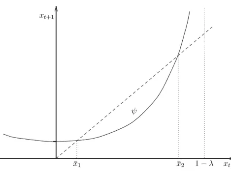
. The graph of the function à is illustrated in Figure 1.

Notice that e

0 requires that x

1

¸. Figure 1 also shows two steady states x

< x

. Because of (15), the associated growth rates are °

> °

. The steady state with the higher growth rate (with the lower bond share) is asymp- totically stable and the other steady state is unstable.

Both steady states have

7Notice that in our model there in no indeterminacy since the initial bond sharex0does not depend on expectations. This is a consequence of our assumption that neither savings nor the coe±cient of the Clower constraint ¸are in°uenced by in°ation expectations. Compare also with Schreft and Smith (1997, p. 175).

8

.. .. .. .. .. .. .. .. .. .. .. .. .. .. .. .. .. .. .. .. .. .. .. .. .. .. .. .. .. .. .. .. .. .. .. .. .. .. .....................................................................................................................

.. .. .. .. .

.. .. .. .. .. .. .. .. .. .. .. .. .. .. .. .. .. .. .. .. .. .. .. .. .. . ...... .............................................................................................................................................................................................

.................

..

...

...

...

...

...

1¡¸ xt

Ã

¹

x1 x¹2

xt+1

Figure 1: Steady states in the case of constant money growth.

a positive level of government debt provided that the equation Ã(x)

Ã(0) = x has a positive solution and that Ã(0) > 0. These conditions are ful¯lled if

(1

¸)

® + ½¾

> f

(a) and q >

µ

1

1

¹

¶

¸

1

f

(a)a f (a)

¶

:

For instance, there are two positive steady states if the uncertainty (or risk aver- sion) and the ¯scal share are not too low. A higher level of government spending or a lower money growth rate shift the graph of à upwards, increase x

and de- crease °

. Thus, ¯scal policy a®ects growth negatively, but money growth has a positive impact on growth. Because of (10), the bond return increases and the equity premium falls which shifts savings from equity to bonds and reduces growth. A further consequence is that the equity premium and the growth rate are positively related. Notice, however, that the comparative statics e®ects on the other (unstable) steady state are opposite.

It remains to check whether the condition R

> R

is satis¯ed in the steady state. Using (10) and (12), this condition is satis¯ed in a steady state if

f

(a)

½¾

® ° > 1

¹ ° . (17)

If the government debt is positive in the stable steady state, we have °

< °

<

(1

¸)®, and therefore (17) holds in both steady states whenever (17) is satis¯ed for ° = (1

¸)®. If the production function is Cobb-Douglas, f (a) = ca

, a

9

su±cient condition for (17) to hold in both steady states is that f(a)

a

º 1

1

¸ + (º

1) 1

¹

¶

> ½¾

.

Necessary for this condition to be ful¯lled is that the term in the brackets is positive which is the case when the money growth rate is larger than (1

¸)(1

º)=º and which is for sure satis¯ed when º

1=2.

Finally, we consider the situation of a zero nominal interest rate in which consumers are indi®erent between holding money and bonds. Unlike the model of Hahn and Solow (1995, Chapter 2), our economy has generically no steady state with that feature. To see this, notice that in this case the dynamical system is described by (9), by

m

¹m

= R

= R

= f

(a)

½¾

® e

e

(18)

and, using (8) and (18), by m

¹m

b

+ q f(a)

a e

= b

+ m

µ

1

1

¹

¶

. (19)

Again, these three equations are homogenous of degree one in (b; m; e) and they can be reduced to two equations using the variables °

= e

=e

, ¯

= b

=e

and º

= m

=e

. (18) yields

°

º

¹º

= f

(a)

½¾

® °

, (20)

(19) becomes

°

º

¹º

¯

+ q f(a)

a = ¯

°

+ º

°

1

1

¹

¶

, (21)

and (9) is

º

+ ¯

+ 1 = ®

°

. (22)

(20) de¯nes a unique stationary growth rate by

° = f

(a)

1

¹ + ½¾

®

¶¡1

. (21) implies that a steady state has to ful¯ll

q f (a) a = °

µ

1

1

¹

¶¡

¯ + º

.

10

But this latter condition is in general not compatible with (22) since this would require that

q f(a) a =

µ

1

1

¹

¶

(®

°) ,

which can only hold true for very particular parameter constallations (for instance if q = 0 and ¹ = 1 as in the model of Hahn and Solow (1995), but not under more general policy speci¯cations).

The results of this section are summarized as follows.

Proposition 2

Under constant money growth, there are no or two steady states in which consumers are liquidity constrained. The steady state with the higher growth rate is asymptotically stable, and the other steady state is unstable. The growth rate and the equity premium at the stable steady state are higher if money growth is faster or if the ¯scal share is lower. An equilibrium with portfolio indi®erence generally does not exist.

3.2 Fixed Money{bond Ratio

We assume here along the lines of Schreft and Smith (1998) that the monetary authority stabilizes the money supply relative to the level of public debt in the economy. That is, it ¯xes the ratio of bonds to money, b

=m

= · for all t: Higher levels of · represent an increase in the bond{money ratio and correspond to a tighter monetary regime. Starting with the case R

> R

, m

= ¸®e

and (9) yield

e

= (1

(1 + ·) ¸) ®e

: Therefore

°

= (1

(1 + ·) ¸) ® = ° (23) which means that the growth rate is constant and independent of q and ½¾

: Since the central bank ¯xes the mix of government liabilities (bonds and outside money) over time, ¯scal policy has no e®ect on growth. Furthermore it follows that

x

= ·¸ = x

and thus also x

is constant and independent of q and ½¾

: By (10) the steady- state bond return is

R

= f

(a)

½¾

® ° . (24)

These results imply that a tighter monetary policy (an increase in ·) increases bond supply and the bond return, reduces the equity premium, increases the ration of bonds to capital, and decreases the growth rate. From (8), (10) and m

= ¸®e

R

= (1 + ·) °

f

(a)

½¾

® °

¶

·

q

¸®

f (a)

a °

11

which in equilibrium becomes R

=

µ

1 + · + ½¾

® ·

q

¸®

f (a) a

¶

°

f

(a) ·: (25) This enables us now to check the validity of the assumption that R

< R

: Using (23), (24) and (25) we can restate this condition as

µ

(1 + ·)

1 + ½¾

®

¶

¡

q

¸®

f (a) a

¶

(1

(1 + ·) ¸) ® < (1 + ·) f

(a) :

For given values of the other parameters, this condition can always be ful¯lled by assuming · and/or q big enough. Moreover, in the special case ½¾

= q = 0 and f(a) = ca

it becomes

1 + · > 1

¸

1

º 1

º

¶

which is for sure satis¯ed when º

1=2:

To complete the analysis we also consider the case of portfolio indi®erence, i.e. R

= R

: From (9) we obtain

(1 + ·) m

+ e

= ®e

whereas (8) and (10) yield

µ

f

(a)

½¾

® e

e

¶

(1 + ·) m

+ q f (a)

a e

= (1 + ·) m

:

Setting as before °

= e

=e

and º

= m

=e

these equations can be written as (1 + ·) º

°

+ °

= ®

and

f

(a)

½¾

® °

¶

(1 + ·) º

+ q f (a)

a = (1 + ·) º

°

: Solving for

°

= ® 1 + Â

with Â

= (1 + ·) º

from the ¯rst equation and inserting in the second yields

f

(a)

½¾

1 + Â

¶

Â

+ q f (a)

a = ®Â

1 + Â

:

8When ½¾² = 0, the consumer is risk neutral or there is no uncertainty. This can be considered a limiting case of our setting in which, from (7) and (10), R^E_t = R^B_t , and the consumer's problem can then be written max_mt;bt;etR^M_t m_t+R^B_t (b_t+e_t) s.t. m_t+b_t+e_t· w_t; m_t¸¸w_t; e_t¸0.

12

Finally solving for Â

we obtain Â

=

³

f

(a)

Â

+ q

®

f

(a)

Â

q

= Á

Â

:

To explore the existence of steady states let us start with the case ½¾

= q = 0:

Then  = 0 is one steady state and, since Á (Â)

as Â

®=f

(a), an additional positive (unstable) steady state exists if Á

(0) < 1. In the special case f(a) = ca

this means º < 1=2. Then, as q is slightly increased, Á (0) > 0 and a stable positive steady state  emerges. This remains true when ½¾

is slightly increased, too. However, this steady state is only an equilibrium of our model if also the liquidity constraint m

¸®e

is satis¯ed. This constraint means that

Â

¸ (1 + ·) 1

¸ (1 + ·) ,

which can be satis¯ed, if at all, only when · is small enough. That is, only a su±ciently loose monetary policy may give rise to a steady state in which the nominal interest rate is zero and in which consumers are portfolio indi®erent. In any way, whenever such a steady state exists, it is clear that a variation in · does not change  and therefore does not change ° either. In conclusion we thus have:

Proposition 3

Under a ¯xed bond{money ratio b

=m

= ·; there is at most one equilibrium in which consumers are liquidity constrained and which must be a steady state. In such an equilibrium a tightening of the monetary regime (i.e. a higher ·) decreases the growth rate, while ¯scal policy does not a®ect growth. If the monetary regime is su±ciently loose, steady states in which consumers are portfolio indi®erent may also exist, but in these steady states the growth rate is independent of ·:

3.3 Interest Rate Targeting

In this case the central bank intends to ¯x the nominal interest factor I

at a value I > 1 for all t. Since I = R

=R

, consumers are liquidity constrained, m

= ¸®e

. Equation (8) now becomes

µ

f

(a)

½¾

® °

¶

b

+q f (a)

a e

= b

+¸®e

1 I

µ

f

(a)

½¾

® °

¶

¸®e

: Setting again x

= b

= (®e

), dividing by e

and using (15) yields

¡

f

(a)

½¾

(1

¸

x

)

x

1

¸

x

+ q f(a)

a

13

= ®x

+ ¸®

1 I

µ

f

(a)¸

1

¸

x

½¾

¸

¶

:

Solving for x

we obtain x

= 1

®

f

(a) x

+ ¸=I

1

¸

x

½¾

x

+ q f(a) a

¸

µ

® + ½¾

I

¶¶

:

The graph of this function is qualitatively the same as the one shown in Figure 1. Both steady states have a positive level of government debt if

(1

¸)

® + ½¾

> f

(a)

1 + ¸

(1

¸) I

¶

and q > ¸a f(a)

µ

® + ½¾

I

f

(a) (1

¸) I

¶

hold. This is for example true when the uncertainty/risk aversion and the ¯s- cal share are high enough. Moreover, higher uncertainty or risk aversion and a lower level of government spending shift the curve downwards decreasing x

and increasing °

. Regarding the e®ect of a change in the nominal interest rate, it can be obtained from

@x

@I = ¸

®

½¾

f

(a) 1

¸

x

¶

1 I

:

For small uncertainty/risk aversion this derivative is negative implying that an increase in I decreases x

and increases °

whereas for large ½¾

the e®ect is reversed. If the uncertainty and risk aversion are low, the increase in the nomi- nal interest rate is accompanied by a larger increase in the in°ation rate which lowers the real interest rate and raises capital investment. On the other hand, if uncertainty and risk aversion are large, the in°ation rate increases less than the nominal interest rate, and so the real interest rate increases as well which a®ects growth negatively. We have therefore obtained the following result.

Proposition 4

Under interest rate targeting there exist no or two steady states.

The steady state with the higher growth rate is asymptotically stable. A decrease in the ¯scal share increases the growth rate and the risk premium. The e®ect of the nominal interest target on growth is positive when uncertainty or risk aversion is small whereas it is negative for uncertainty and risk aversion large.

3.4 In°ation Targeting

Under in°ation targeting the central bank aims to have R

= R

for all t and R

> 0 predetermined. Proceeding as in the previous section, the case R

> R

yields

¡

f

(a)

½¾

(1

¸

x

)

x

1

¸

x

+ q f (a)

a

14

= ®x

+ ¸®

µ

1

R

®(1

¸

x

)

¶

and therefore x

= 1

®

µ

f

(a)x

+ ¸R

1

¸

x

½¾

x

+ q f(a) a

¸®

¶

:

The graph of this function is again as in Figure 1. Both steady states involve positive government debt if

(1

¸)

® + ½¾

> f

(a) + ¸R

1

¸ and q > ¸a f(a)

µ

®

R

1

¸

¶

hold. As before, these conditions can be ful¯lled if uncertainty, risk aversion and government consumption are large enough. Regarding the comparative statics properties of the steady states, they are analogous to the case of interest rate targeting. The only di®erence is that now an increase in the in°ation rate (a lower R

) unambiguously lowers the real interest rate and increases the growth rate.

When is it true that in a steady state R

> R

? From (10) a necessary con- dition is f

(a) > R

. This means that too low an in°ation rate is unsustainable on a steady-state growth path with liquidity-constrained consumers. Portfolio indi®erence, on the other hand, requires from (10) for the growth rate to be constant with value

° =

f

(a)

R

®

½¾

(26)

which cannot be ful¯lled when ½¾

= 0 (unless R

happens to be equal to f

(a)).

However, also when ½¾

is positive, steady states with R

= R

in general do not exist. To see this, set as earlier ¯

= b

=e

and º

= m

=e

. Then (9) yields

º

= ®

°

1

¯

, (27)

whereas (8) implies

q f (a)

a = (¯

+ º

) °

R

(º

+ ¯

):

Inserting for º

we obtain q f (a)

a = ®

°

R

®

°

1

¶

which shows that an equilibrium can only exist if R

ful¯ls this equation. But under in°ation targeting R

is a predetermined magnitude, and thus a steady state with portfolio indi®erence generally does not exist.

We summarize the results on in°ation targeting as follows.

15

Proposition 5

Under in°ation targeting there are no or two steady states with liquidity-constrained consumers. The steady state with the higher growth rate is asymptotically stable. A higher in°ation target or a lower ¯scal share increase the growth rate and the risk premium. Equilibria with portfolio indi®erence generally do not exist.

Notice that the results of Sections 3.3 and 3.4 are compatible with those of 3.1 and 3.2. Indeed, denoting with ¹ the steady-state increase in the nominal money stock, it is related to inflation by ¹ = °=R

. An increase in the in°ation rate increases ° and hence ¹. Thus ¹ and ° are correlated positively, as was predicted in the case of constant money growth. Regarding the ratio of bonds and and the money stock · = b=m, from (14) and m

= ¸®e

it is equal to (1

¸

°=®) =¸: An increase in the in°ation rate increases (in the stable steady state) ° and hence diminishes ·, meaning that · and ° are inversely correlated as stated in section 3.2.

4 Adaptive Expectations

We have shown in the previous section that our model exhibits in most cases two steady states in which consumers are liquidity constrained, and we argued that the steady state which is stable in the perfect foresight dynamics is the relevant one, whereas the unstable steady state whose policy features are opposite is of mi- nor importance. We give now further support to this argument by showing that a steady state which is stable under perfect foresight is also stable under adaptive expectations, and vice versa. Thus our model predicts the same outcome in the forward perfect foresight dynamics as under learnung with adaptive expectations.

This result contrasts to the result of Grandmont and Laroque (1986) who show that, under their assumptions, stability in the backward perfect foresight dynam- ics relates to stability in the actual learning dynamics.

The following analysis is restricted to the case of constant money growth, but we believe that similar results can be obtained with an in°ation targeting or an interest rate targeting policy.

Since the distribution of the capital return is the same in every period irre- spective of the state of the economy, we assume that the consumer has learned this distribution perfectly and forecasts correctly its mean and variance as given by (7). However, the consumer does not perfectly foresee the in°ation rate and we assume that he holds in period t an in°ation forecast R

. At the nomi- nal interest rate I

his forecast of the real interest rate is then R

= I

R

. A temporary equilibrium in period t , given an in°ation expectation R

, is a

9In Grandmont and Laroque (1986) the law of motion of the economic system is of the type X_t =F¡

X_t+1^e ¢

whereas our system is of the form X_t = F(X_t¡1; X_t^e). Expectations of the future stateX_t+1^e do not enter our temporary equilibrium map, cf. footnote 7.

16