RESH Discussion Papers No. 2 / 2020

RESH Discussion Papers

No. 2 / 2020

Tobias A. Jopp

A Happiness Economics-Based Human

Development Index for Germany (1920-1960)

FAKULTÄT FÜR PHILOSOPHIE, KUNST-, GESCHICHTS- UND GESELLSCHAFTSWISSENSCHAFTEN

i

REGENSBURG ECONOMIC AND SOCIAL HISTORY (RESH) Discussion Paper Series

Edited by

Prof. Dr. Mark Spoerer and Dr. Tobias A. Jopp

Processed by Dr. Tobias A. Jopp

University of Regensburg

Faculty of Philosophy, Art History, History and Humanities Department of History

Chair for Economic and Social History

The RESH Papers are intended to provide economic and social historians and other historians or economists at the University of Regensburg whose work is sufficiently intersecting with economic and social history with the possibility to circulate their work in an informal, easy-to-access way among the academic community. Econo- mic and social historians from outside the University of Regensburg may also consider the RESH Papers as a means to publish informally as long as their work meets the academic standards of the discipline. Publishable in the RESH Papers is the following: Work in progress on which the author(s) wish to generate comments by their peers before formally publishing it in an academic journal or book; and English translations of already published, yet non-English works that may be of interest beyond the originally targeted (German, French, and so on) audience.

Authors interested in publishing in the RESH Papers may contact one of the editors (Mark.Spoerer@ ur.de; Tobias.Jopp@ur.de).

Cover page photo on the left: Café Kranzler um 1925. Source: https://www.dhm.de/lemo/bestand/objekt/cafe-kranzler-um- 1925.html.

Final page photos: Own material.

ii

A Happiness Economics-Based Human Development Index for Germany (1920-1960)

Tobias A. Jopp

Abstract: The United Nations’ Human Development Index (HDI) has become an important tool for measuring and comparing living standards between countries and regions. However, the HDI has also attracted a fair share of conceptual criticism. Starting from Andrea Wagner’s historical estimations of a HDI for Germany in the interwar and early post-war period, we take up part of that criticism by implementing three essential modifications to the mode of calculation. We test how far they alter our picture of the relative living standard in the Weimar Republic, the Third Reich, and the Federal Republic of Germany. First, we replace the arithmetic mean by the geometric mean, which is said to solve the problem of perfect substitutability; second, we extend the HDI by an additional fourth dimension measuring economic and political freedom – an important, though neglected, dimension; and third, as the perhaps most crucial conceptual intervention, we develop weighting schemes for the partial indices that are theoretically backed by happiness economic research. Thus, we challenge the common, but arbitrary fundamental assumption that all partial indices receive equal weights. Our results show that the HDI for Germany reacts very sensitively to conceptual interventions, making it difficult to use it for the intertemporal and international comparison of living standards. We also find that the proposed modified HDIs allow for a re-evaluation of the living standard in interwar Germany; and in contrast to what the reference estimations on the HDI for Germany say, there is a profound discontinuity between the Third Reich and post-war Germany in terms of living standards.

Keywords: Germany, freedom, weighting, happiness research, happiness economics, Human Development Index, living standard

JEL classification: I31, N34, N94, O11

Acknowledgements: I am deeply indebted to Mark Spoerer, Jochen Streb, and two anonymous referees for their invaluable comments on the original manuscript.



This discussion paper is a translation of a journal article originally written in German. Possible revisions to the original version (inclusion of new literature and/or new evidence) are indicated as such. The original publication is: Tobias A. Jopp (2017): Ein glücksökonomisch modifizierter Human Development Index für Deutschland (1920-1960), in:

Please cite the original publication along with this discussion paper.



Contact: Dr. Tobias A. Jopp, University of Regensburg, Department of History, Economic and Social History,

93040 Regensburg; email: Tobias.Jopp@ur.de.

1

A Happiness Economics-Based Human Development Index for Germany (1920-1960)

1. Objective

What standard of living did societies maintain at different times depending on geographical, institutional and cultural parameters? How did some societies succeed in generating sus- tainable economic growth and broad-based prosperity, and why did others not? How do we measure living standards in the first place, and are the measures that prove suitable for de- scribing today's societies also applicable to earlier societies? Monetary indicators such as domestic product per capita or real wages still play a central role in answering these core questions of economic history. What is unsatisfactory, however, is that their application draws attention to the material dimension of living standards, while other important dimen- sions are not – or at best indirectly – captured (e.g. Landes 1999; Pierenkemper 2005: 41-7;

Maddison 2008; Allen 2011; Acemoglu/Robinson 2012; Hesse 2013: 41; and Broadberry et al. 2015).

To compensate for this weakness, further measures have been established in the liter- ature on economic history, and social sciences, in general. The indicators for the biological standard of living or psychological measures, but also multidimensional welfare indices, are of particular interest here. The latter include, for example, the Human Development Index (HDI), which has been regularly calculated by the United Nations since 1990 (e.g. Dasgup- ta/Weale 1992; Steckel/Floud 1997; Baten 2003; Pierenkemper 2005: 48-50; Steckel 2008;

Fleurbaey 2009; Deaton 2013; aus dem Moore/Schmidt 2013; Craig 2016). Constructed in its original form as a measure of deprivation of essential freedoms and opportunities improv- ing individual welfare, it measures living standards in the dimensions of health, education and access to material resources (or lack thereof). These sub-dimensions were measured by the variables life expectancy at birth (LE), adult literacy rate (AR) and logarithmic per capita income (PKE). For the purpose of aggregation, the values observed for any country i were normalized to the interval from zero to one. To do so, the minimum and maximum values (i.e. the worst and best values) of the variables to be observed in the country cross-section for the corresponding year t were used; expressed in a formula (Rao 1991; Anand/Sen 1994):

(1) HDI

= 1– _



 





 

 







 

 

 







 

 

 







 3

) ( ) (

) ( )

( ) (

) ( )

( ) (

) (

t t

it t

t t

it t t

t

it t

PKE Min PKE

Max

PKE PKE

Max AR

Min AR

Max

AR AR Max LE

Min LE

Max

LE LE

Max .

2 This formula has prompted a lively discussion of the HDI’s pros and cons. The conceptual criticism was particularly directed at the following problem areas (Raworth/Stewart 2005; ul Haq 2005: 135-6; Stanton 2007; Herrero et al. 2010: 4-5; Herrero et al. 2012): First, the se- lection of the sub-dimensions covered (e.g. Dasgupta/Weale 1992: 119; Desai 1991; Streeten 1994: 236; Salas-Bourgoin 2014; Ray 2014); for example, are political freedom(s) and civil rights or sustainability aspects not missing in the consideration? Second, the choice of ap- propriate indicators (e.g. Dasgupta/Weale 1992: 119; Streeten 1994: 236); are the chosen variables really the best proxy variables? Third, the choice of minimum and maximum values as the basis for normalization (e.g. Trabold-Nübler 1991: 239); instead of varying in the cor- responding cross section of countries, should they not better be constant and represent goalposts?

Fourth, the additive linking of the sub-indices via the arithmetic mean (e.g. Hop- kins 1991: 1471; Desai 1991: 356; Sagar/Najam 1998: 251-2; Mazumdar 2003: 540); is the assumption of perfect substitutability between very different sub-dimensions implicit in the simple arithmetic mean theoretically really viable? Fifth, the equal weighting of the sub- dimensions with one-third each (e.g. Kelley 1991: 318-9; Srinivasan 1994; Chowdury/Squire 2006; Ravallion 2012: 9); is it theoretically justifiable that all sub-dimensions have the same significance for human development, or do we have simply to accept the normative dictum that this should be the case? Sixth, the inclusion of distributional issues (e.g. Sagar/Najam 1998: 263; Trabold-Nübler 1991; Hicks 1997; Martinez 2012: 533); should greater inequality in income, health and education not have a negative impact on the level of a country’s HDI and ranking across countries? Seventh, treatment of the income variable (e.g. Sagar/Najam 1998: 263); should we not “write off” income according to the idea of diminishing marginal returns? If so, how we should we do that? Finally, eighth, the overarching question related to the weighting procedure whether a multidimensional welfare index offers surplus value over the dashboard approach, according to which as many individual indicators as possible are interpreted separately, albeit comparatively (e.g. McGillivray 1991: 1467; Fleurbaey 2009: 1055; Ravallion 2012: 6-10).

The United Nations had already reacted to some criticisms at an early stage (Jahan 2004: 155; Stanton 2007: 16-20). The following modifications had already been implemented when economic history finally discovered the HDI in 1997: on the one hand, there had been

1

A change in the HDI from one year to the next can thus be generated solely by varying minimum and maxi-

mum values, which makes interpretation difficult.

3 a change of perspective; since 1991 human development had no longer been evaluated from the point of view of “deprivation” but rather from that of “achievement”. On the other hand, the education sub-dimension was covered by another variable, namely, from 1991 onwards, first by the number of years of intermediate school attendance and then, from 1995 onwards, by the gross enrolment rates in primary, secondary and tertiary educational institutions. Moreover, from 1991 onwards, no longer was logarithmic income used over the entire range of values observed, but it was depreciated in sections beyond a threshold of

$5,000 – a kind of minimum standard – using a special formula. Finally, from 1995 onwards, the observed values were standardized on the basis of fixed minimum and maximum values instead of minimum and maximum values that changed from year to year (Jahan 2004: 155- 6).

Historical HDI studies published since 1997 provide a good indication of the extent to which the HDI has been developed since and of the weaknesses still critically discussed. The first four were published in a collective volume edited by Robert Steckel and Roderick Floud (1997) on the question of what effect industrialization has had on the extended standard of living. Investigated were the United States of America in the period 1800-1970 (Cos- ta/Steckel 1997), Great Britain 1700-1980 (Floud/Harris 1997), Sweden 1820-1965 (Dandberg/Steckel 1997), and Germany 1871-1950 (Twarog 1997). The studies’ main chal- lenges were to adjust the minimum and maximum values to historical conditions and to se- lect appropriate indicators given the difficult data situation. In addition to the classic com- ponents of the HDI, the variables height and infant mortality were also used as indicators of health, while the education index had to be reduced to the literacy rate in all cases (Cos- ta/Steckel 1997: 71; Floud/Harris 1997: 115; Sandberg/Steckel 1997: 148-9; Twarog 1997:

322-324). Following Costa and Steckel’s assessment, the historian’s benefit of using the HDI precisely results from the fact that the HDI is a “distance measure”, while the growth rate of per capita income is a “measure of the speed” of an adjustment process; i.e., both measures principally are complementary (Costa/Steckel 1997).

Since then further historical studies applying the HDI have been published: Besides the

traditional HDI, Crafts (1997a) calculated HDIs for Great Britain between 1760 and 1850 that

included distributional and gender aspects and also the Dasgupta-Weale Index as an alterna-

tive multidimensional measure of welfare that explicitly takes into account political free-

doms and civil rights. Crafts (1997b, 2002) also calculated the classic HDI for five years (1870,

4 1913, 1950, 1973, 1992/1999) and a cross-section of countries that essentially covers the western states but also a few selected Latin American and Asian countries. His recalculation of the historical HDI values from 2002 served to incorporate the return to logarithmic in- come over the entire value range. Wagner (2003, 2007, 2008) calculated and discussed four HDI variants for Germany in the period 1920 to 1960, namely the classical HDI, a Germany- specific Development Index (DDI) expanded by additional variables such as the unemploy- ment rate and infant mortality, a Gender-related Development Index and a HDI at the re- gional level for the analysis of regional differences in living standards. It is particularly note- worthy that Wagner calculated the DDI for all years between 1920 and 1939 as well as 1949 and 1960 and was thus able to draw a detailed picture of the development of living stand- ards, particularly in the turbulent interwar period. Astorga, Berges and Fitzgerald (2005) es- timated the classic HDI (education index reduced to the literacy rate) for Latin America and the years 1900, 1950 and 2000, and Escudero and Pérez Castroviejo (2010) presented esti- mates of the classic HDI for a specific social group, namely Spanish miners (1876-1936).

With Prados de la Escosura (2010, 2013, 2015a, 2015b), there are also four studies that take up and elaborate on Crafts’ approach. Specifically, Prados de la Escosura’s estimates covered almost all countries of the world and the period from 1870 to 2007 (in ten-year steps). Un- like all previous studies, Prados de la Escosura calculated the HDI based on the multiplicative linkage of the sub-indices, i.e. as a geometric mean. This corresponds to the United Nations’

modification of the HDI of 2010 in response to the ongoing discussion on the problem of the additive linking of the sub-indices. Another special feature is the application of a convex achievement function to the sub-indices for health and education. As a result, a change in the corresponding variables has greater weight the higher the already achieved level.

Final- ly, Felice and Vasta (2015) calculated the classical HDI, also based on the geometric mean, for the Italian regions between 1871 and 2007 using four variables. But like Prados de la Es- cosura (and therefore for reasons of data availability) the authors continued to use literacy and school attendance rates in the education index. It should be noted that in 2010 the United Nations began measuring education through the variables average years of schooling and expected years of schooling.

2

It remains unclear whether the authors already use the geometric mean instead of the arithmetic mean, as done by the United Nations since 2010.

3

This reflects the view that highly developed countries may have lower marginal returns on health goods than

less developed ones, making it more difficult for them to further improve once a high level is achieved.

5 This cursory overview shows that the classic HDI as an alternative measure of the standard of living has raised economic historians’ interest. However, it has also shown that, in addition to the desire to derive estimates of historical HDIs as far as possible in accord- ance with the latest conceptual standards, economic historical research can provide meth- odological suggestions as to how the HDI can be improved in application (e.g. with regard to the choice of variables, the regional concept and the weighting of achievements). This is the starting point of this article: The aim is to modify Wagner’s (2003, 2006) detailed estimates of a Germany-specific Development Index (DDI) for the period 1920-1960 in three points and to examine to what extent this changes the picture of the development of the extended standard of living in Germany. The first modification is to apply the geometric mean to the DDI, since the multiplicative linkage of the sub-indices is now accepted as the more theoreti- cally meaningful. The two other modifications – on the one hand, adding the sub-dimension of political and economic freedom to the DDI and, on the other hand, implementing a weighting scheme rooted in happiness economics – take up two points that are still contro- versial, namely the selection of sub-dimensions and the theoretically problematic one-third or equal weighting of the sub-indices. With the latter two modifications, an attempt is made to react to the fundamental criticism of the HDI concept, also expressed by economic histo- rians themselves. Wagner (2003: 181) herself conceded: “It would be desirable to derive individual welfare components and their weights from the preferences of individuals as de- termined by surveys. However, no such data exist for the period under study.”

The ap- proach proposed in this study shows how, despite the lack of adequate data, a preference- oriented weighting scheme can be derived by drawing on current findings of happiness eco- nomics research. Wahl’s (2013) recent study on the standard of living in the Third Reich shows that happiness economics have potential for application in economic history research.

The following section briefly discusses Wagner’s DDI, which forms the starting point for this study; in the third section, the proposed modifications are discussed or, respectively, made plausible on a formal level. The empirical results are presented in the fourth section.

The fifth section concludes.

4

Author’s translation of the German original:

6 2. Point of departure: Wagner’s Germany-specific development Index

Wagner’s DDI was constructed to serve as a basis for a detailed intertemporal analysis of the standard of living in Germany between 1920 and 1960; compared to Wagner’s classic HDI, it was enriched by additional indicators in the indices of material well-being and health, name- ly the unemployment rate, life expectancy at the age of five (instead of life expectancy at birth), and infant, child and maternal mortality. Table 1 shows the minimum and maximum values for these and all other variables applied by Wagner (2008: 39-47) and which are sub- sequently retained.

Table 1: Components of Wagner’s DDI and their standardization

Component Lower bound Upper bound

(1) Gross domestic product per capita (1990 PPP $) log(100) log(40.000)

(2) Unemployment rate 100 0

(3) Life expectancy at birth 25 85

(4) Life expectancy at age 5 45 75

(5) Infant mortality 280 0

(6) Child mortality 28 0

(7) Maternal mortality 100 0

(8) Tertiary enrolment rate (among the 20 to 25 year old) 0 100 Sources: Wagner (2008: 260, 270).

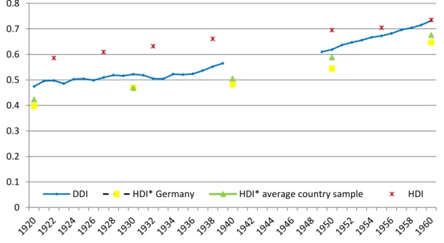
Figure 1: The development of the standard of living in Germany according to Wagner, 1920- 1960

Sources: Wagner 2008: 259, 261-3, 271.

0 0.1 0.2 0.3 0.4 0.5 0.6 0.7 0.8

DDI HDI* Germany HDI* average country sample HDI

7 Figure 1 shows the development over time of the HDI measures designed by Wagner for Germany as a whole. The DDI starts at an index value of about 0.48 in 1920 and rises to an index value of about 0.74 in 1960. With regard to the increase in the trend, two phases can be distinguished, namely the phases 1920 to 1935 and 1936 to 1960; in the latter, the stand- ard of living in Germany rose more strongly than before and also increased evenly. According to Wagner, the marked increase in the DDI between 1936 and 1939 was due to the strong growth in per capita income, which more than compensated for losses in the areas of health and education. This shows that the National Socialist economic miracle, as widely accepted, was a “de-formed economic miracle”. In comparison, however, 1923 (peak of inflation and Franco-German tensions), 1926 (stabilization crisis of the “Golden Twenties”), 1929 (begin- ning of the Great Depression) and 1932/1933 (peak of the Great Depression and regime change/normalization shock) can be identified as years in the first phase in which the DDI even temporarily declined, but never fell below the initial level of 1920. The standard of liv- ing in the Weimar Republic peaked in 1930; and, after 1933, the HDI never fell below the level of approx. 0.53 index points.

In addition to the DDI, Wagner also calculated the classic HDI with four variables (life

expectancy at birth, literacy rate, gross school attendance rate, per capita income) and the

HDI*, which, for reasons of data availability, only includes the rate of university attendance

(i.e. students as a percentage of the 20 to 25-year-olds) as a measure of education. The lat-

ter serves as the basis for a comparison of Germany with selected European countries,

namely Denmark, France, Great Britain, Italy, the Netherlands, Norway, Sweden and Switzer-

land. Wagner calculated both measures for selected reference years. Compared with the

DDI, the traditional HDI implies a much faster increase in living standards during the interwar

period and a slower increase after 1949, while the trend in the HDI* is in line with that of the

DDI. In an international comparison, the standard of living in Germany ranged slightly below

the European average until 1930 (Wagner 2008: 60-62 and Appendix 1). It should also be

noted that for all three measures the gap between 1939 and 1949/50 is relatively small

(about 0.05 index points each), so that it can be concluded that in terms of extended living

standards there would have been continuity between the Third Reich and the Federal Re-

public rather than between the Weimar Republic and the Federal Republic. A brief review of

the data used to measure the extent of economic and political freedom as the basis of an

8 additional freedom index, taken from work by Prados de la Escosura and Marshall, Gurr and Jaggers (Prados de la Escosura 2016; Marshall et al. 2014), is done in Section 4.

Among other things, I will show that the HDI/DDI generally reacts very sensitively to subtle changes in the calculation rules, rendering its use as a measure of intertemporal and international welfare comparison problematic from a purely technical perspective. However, if one does not want to dispense with the HDI/DDI in the (economic history) discussion, one must at least be aware of its sensitivity to both minor and major modifications. Subject to this aspect, it is demonstrated that, on the basis of the justified modifications, a reassess- ment of the development of living standards in detail, especially before 1939, is indeed in order.

3. Proposed modifications of the Germany-specific Development Index

3.1. Modification one: Use of the geometric mean

Since 2010, the United Nations have calculated the HDI as the geometric mean of the partial indices, i.e. formally as

(2) HDI

=

1

max min



min

 





 









j

j j

j ijt

X X

X

X ,

where index j denotes the sub-indices (J = 1, 2, 3) and indices i and t are already known (see above). In addition to switching to the geometric mean, the most recent modifications of 2010 also include the use of Gross National Product per capita instead of the Gross Domestic Product per capita; partially adjusted goalposts; the use of the variables mean completed school years and expected completed school years as substitutes for the literacy rate and school attendance rate in the education index; and a version of the HDI extended by inequal- ity in all three sub-dimensions and published separately (Beja 2014: 29; Martinez 2012: 533;

Ray 2014: 308).

Switching to the geometric mean was a reaction to the recurring criticism that the ad-

ditive linkage of the sub-indices via the simple arithmetic mean implied perfect substitutabil-

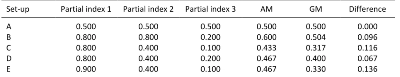
ity between the sub-dimensions. This aspect can be illustrated by simple example. Table 2

9 reports five hypothetical constellations of sub-index values (Ravallion 2012: 202-3; Tofallis 2013: 1329).

If all sub-indices take on the same value, the arithmetic (AM) and geometric mean (GM) do not differ (see constellation A). If, however, the index values are unequal, the geo- metrically averaged HDI (as in principle the geometric mean of any series) is always lower than the arithmetically averaged HDI (see constellations B to E). In particular, the greater the dispersion of the index values, the smaller the geometric mean is in comparison to the arithmetic mean (compare constellations B and C). The use of the arithmetic mean – i.e. the additive linkage – tacitly introduces a certain baseline assumption, namely that, for example, a loss in life expectancy can be fully compensated by a corresponding gain in educational attainment or per capita income. This can be traced in Table 2 by comparing the change in HDI from constellation C to constellation D – an increase of 0.1 index points in sub-index 3 – and from constellation C to constellation E – an increase of 0.1 index points in sub-index 1.

While the arithmetic mean “values” both developments identically (AM equals 0.467 each), the geometric mean “values” the same change that occurs from C towards D more positive- ly, as the change occurs from a lower starting point (GM increases by 0.083 compared to 0.013) and reduces dispersion. In other words, in a sense the geometric mean punishes an improvement in an already strongly positive partial dimension.

Table 2: Does the arithmetic mean even out unequal HDI developments?

Set-up Partial index 1 Partial index 2 Partial index 3 AM GM Difference

A 0.500 0.500 0.500 0.500 0.500 0.000

B 0.800 0.800 0.200 0.600 0.504 0.096

C 0.800 0.400 0.100 0.433 0.317 0.116

D 0.800 0.400 0.200 0.467 0.400 0.067

E 0.900 0.400 0.100 0.467 0.330 0.136

Sources: Author’s own depiction.

The switch in mean is therefore not just a statistical gimmick, as one might think. Overall, the

geometric mean makes it easier to assess the balance of development in the sub-areas of

human development covered. However, it should be noted that the difference between the

arithmetic and geometric mean, as it occurs in constellations B to E, does not automatically

imply a lower standard of living. Rather, the difference must be taken to mean that the ap-

10 plication of the geometric mean reveals a characteristic of the development process that is simply ignored when the arithmetic mean is applied.

3.2. Modification Two: Addition of the “freedom“ dimension

Since the HDI’s introduction, the question has repeatedly been raised as to whether there are other dimensions that should be taken into account in addition to the elementary sub- dimensions of health, education and material prosperity. According to many critics, freedom – both political and economic – is such a further elementary but so far missing sub- dimension (Desai 1991; Dasgupta/Weale 1992:112; Streeten 1994: 236; ul Haq 2005: 135;

Salas-Bourgoin 2014: 36-8). According to Desai (1991: 356), although the HDI indirectly co- vers positive freedoms, this is not enough, especially since negative freedoms are addressed neither directly nor indirectly. Positive freedom means having the formal, and also material, possibility to do something (access to resources!); negative freedom, in contrast, means en- joying protection from restriction or third parties’ (i.e., the state or other individuals) arbi- trary behavior (Chauffeur 2011: 4; MacMahon/Dowd 2014: 66).

The corresponding entry in the Encyclopedia of Public Choice can serve as a starting point for a critical discussion of both concepts of freedom. There it reads (Wu/Davis 2004:

163-4):

“Economic freedom refers to the quality of a free private market in which individ- uals voluntarily carry out exchanges in their own interests. Political freedom means freedom from coercions by arbitrary power including the power exercised by the government. Political freedom consists of two basic elements: political rights and civil liberties. Sufficient political rights allow people to choose their rul- ers and the way in which they are ruled. The essence of civil liberties is that peo- ple are free to make their own decisions as long as they do not violate others’

identical rights.”

It is certainly undisputed that both concepts are fundamentally interwoven and also have a

value for the individual and social standard of living per se (Wu/Davis 2004: 164; Stroup

2007: 52). It is undisputed too, however, that a major challenge is to support these state-

11 ments empirically. Especially with regard to the operationalization of freedom, several prob- lem areas arise, which will be outlined in the following.

The literature emphasizes that economic and political freedom are multidimensional concepts that can only be described in terms of content by whole bundles of variables - i.e.

in the form of freedom indices (Chauffeur 2011: 5-6; Caudill et al. 2000). Apart from variable selection in detail, it is often critically pointed out that freedom indices basically mix two groups of variables, namely on the one hand the group by which the structures or the exist- ence and design of rules (settings/rules of the game) are measured; and on the other hand the group by which the results of action and the degree of enforcement are grasped. Mixing these groups makes the comparative interpretation of the sub-indices or the interpretation of the freedom index itself more difficult (Desai 2005: 190).

Besides, it must also be taken into account that the concept of economic freedom, as used in the relevant literature, is based on the “paradigm of the (free) market economy”, which usually implies strong property protection, stable (i.e. expectation-stabilizing) prices, little or no trade or transaction restrictions and generally a low level of regulation (Wu/Davis 2004: 164; Berggren 2003; De Haan et al. 206: 158). Similarly, the state form of democracy usually serves as a foil for the definition of political freedom; political freedom means being able to freely found and join already existing organizations; to enjoy freedom of opinion, faith and the press as well as the rule of law (subsumed under civil rights/civil liberties); and to be able to participate voluntarily and without restrictions in the political decision-making process, for example by exercising voting rights or seeking public office in the context of an election (subsumed under political liberties) (Wu/Davis 2004: 167; Fabro/Aixalá 2012: 1060;

Desai 2004: 192). With regard to history in general, the question arises as to what extent historical societies, which were rather autocratically shaped and/or possibly heavily regulat- ed, can be meaningfully grasped by freedom indices that are based on the superiority of the (free) market economy and democracy over all other forms of economic and social organiza- tion.

Finally, with regard to a comprehensive concept of freedom, it is not clear what the exact empirical relationship is between economic freedom, political freedom and civil rights on the one hand and freedom and economic growth or individual/societal welfare on the other (Fabro/Aixalá 2012: 1061-3; de Haan/Sturm 2000; Sturm/de Haan 2001; Xu/Li 2008).

Following the Encyclopedia of Public Choice once again, but also positions formulated else-

12 where, there are good reasons to assume that the realization of a high degree of economic freedom presupposes the existence of civil rights, but not necessarily the existence of politi- cal freedom. Rather, we may assume with Friedman „[that] political freedom, once estab- lished, has a tendency to destroy economic freedom“ (Wu/Davis 2004: 164).

Especially with regard to historical applications, this leads to the question of how regimes that offer little or no political freedom actually perform on this point. Did such regimes, and do they generally, offer economic freedom to a degree anyway (Fabro/Aixalá 2012: 1061-3; Aixalá/Fabro 2009)? Moreover, the question of the relationship between freedom of any kind and living standards is by no means trivial, since it is imaginable both that individual/societal welfare has a strictly linear relationship with a particular variable or the freedom index as a whole and that individual/societal welfare is at its maximum when the variable is at an average level (i.e. when there is a non-linear relationship). Could certain state interventions, e.g. to correct for a market failure or to provide a public good, not even be welfare enhancing indi- vidually or collectively (Stroup 2007: 52-54)? In short: What degree of economic and political freedom maximizes welfare with regard to the individual and to society as a whole?

Subject to these problematic points, a freedom index should definitely be considered as an additional component of the DDI, not only against the background of the fundamental criticism of the HDI, but especially against the background of the far-reaching political and economic upheavals during the period under study. This would allow drawing a more accu- rate picture of the development of living standards. With the aim of implementing a concept of freedom that is as comprehensive as possible, two indices for economic and political free- dom available in the literature will be used in the following. One is the recently published Historical Index of Economic Liberty (HIEL) by Prados de la Escosura (2016 2016: 6), which covers the period between 1850 and 2007 and all OECD countries;

and the other is the In- dex of Political Freedom, or Combined POLITY Score (CPS), estimated by the Polity IV Project for the period between 1800 and 2013 (Marshall/Gurr/Jaggers 2014: 16-7).

5

This statement is attributed to Milton Friedman. It is based on the idea that politicians are fixated on maxim- izing votes and securing re-election in the short term and therefore tend to pursue policies that benefit their voters by redistributing economic/political privileges (rent-seeking). One could also extend the causal chain by arguing that a high degree of economic freedom promotes (financial) inequality to an extreme degree, which in turn perverts the political decision-making process to such an extent that economic freedoms are reduced for certain groups and further expanded for others.

6

See also pages 6 to 22 for an in-depth discussion of the components of the HIEL. The Economic Freedom

Index of the Fraser Institute, which serves as a starting point for Prados de la Escosura, “only” goes back to

1970.

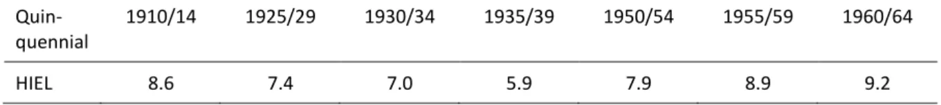
13 Prados de la Escosura (2016: 2-3, 13-4) addressed the above-mentioned problematic points in detail when developing the HIEL. As a result, the HIEL combines four dimensions of economic freedom, namely the quality of the legal system (legal structure and property rights), the stability of the monetary system (money), the unrestricted mobility of goods and capital (international trade) and the degree of regulation; it follows the dictum that a coun- try can be regarded as economically free “[...] insofar as privately owned property is securely protected, contracts enforced, prices stable, barriers to trade small, and resources mainly allocated through the market” (Prados de la Escosura 2016: 2, 11). Table 3 reports the HIEL values for Germany. As can be seen from the table, the HIEL takes on values between zero and ten, with higher values implying a greater degree of economic freedom.

Table 3: The values of the Historical Index of Economic Liberty for Germany

Quin- quennial

1910/14 1925/29 1930/34 1935/39 1950/54 1955/59 1960/64

HIEL 8.6 7.4 7.0 5.9 7.9 8.9 9.2

Sources: Prados de la Escosura (2016: 23-4).

While Germany ranks in the middle of the distribution before the First World War (mean value over 20 countries: 8.6), it is at the bottom of the distribution in the interwar period and in the upper distribution after 1945; in the period 1930/34 only Italy (6.9) and Portugal (6.5) are behind Germany, and in the period 1935/39 only Italy (5.9) and Spain (3.0) (Prados de la Escosura 2016: 23-4).

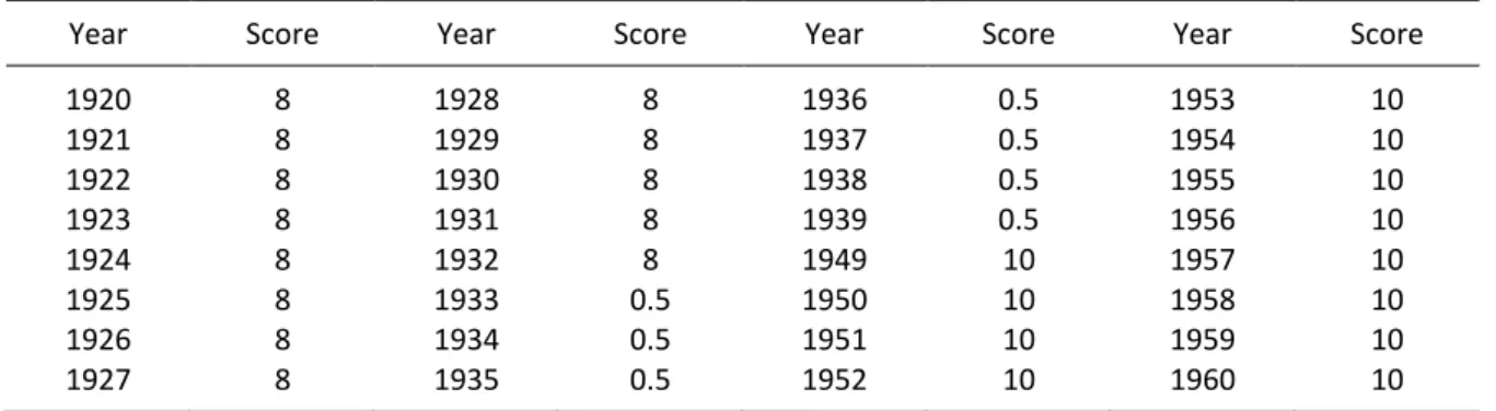
The Center for Systemic Peace’ CPS is a combination of two sub-indices, namely an

index measuring the degree of institutionalized democracy and an index measuring the de-

gree of institutionalized autocracy. Among other things, it measures whether the general

population has the institutionalized opportunity to express preferences for alternative politi-

cal approaches or to participate in the political sphere. While the former index takes on val-

ues between zero and plus ten (low to high democracy), the latter ranges from minus ten to

zero (high to low autocracy). Thus the CPS ranges between minus ten and plus ten, with

changes in integer steps (Marshall/Gurr/Jaggers 2014: 14-18). In order to establish compa-

rability with the HIEL, the CPS was rescaled to the interval from zero to ten (with changes in

steps of 0.5). Table 4 presents the adjusted values of the CPS used below.

14 Table 4: The Combined POLITY Score’s values for Germany

Year Score Year Score Year Score Year Score

1920 8 1928 8 1936 0.5 1953 10

1921 8 1929 8 1937 0.5 1954 10

1922 8 1930 8 1938 0.5 1955 10

1923 8 1931 8 1939 0.5 1956 10

1924 8 1932 8 1949 10 1957 10

1925 8 1933 0.5 1950 10 1958 10

1926 8 1934 0.5 1951 10 1959 10

1927 8 1935 0.5 1952 10 1960 10

Sources: http://www.systemicpeace.org/inscr/p4v2014.xls, 11.11.2015.

Figure 2: A proposal for an unweighted freedom index as part of the DDI

Sources: Author’s own depiction. For the data sources, see Tables 3 and 4.

In order to arrive at a historical freedom index, the HIEL and the CPS were first linked using the simple – i.e. unweighted – arithmetic mean.

Figure 3 shows the course of the freedom index in its basic form. The basic rule is that only if both dimensions of freedom are equally pronounced we can speak of a high degree of freedom overall. Of course, the HIEL and the CPS can also be linked via the geometric mean and, in principle, can be weighted unequally (see also Figure 3 and Section 4.2).

7

The following goalposts were used: 0 and 10 (political freedom), 2.7 and 10 (economic freedom).

8

The problem of the lack of data for the HIEL for the period 1920 to 1923 was solved as follows: Against the background of the crisis-ridden immediate post-war years (including hyperinflation, foreign trade re- strictions), it makes no sense to take the mean value for the phases 1910/14 and 1925/29. Instead, a value of 7.0 was applied, as Prados de la Escosura calculated for the phase in which the world economic crisis oc- curred.

0.0 0.1 0.2 0.3 0.4 0.5 0.6 0.7 0.8 0.9 1.0

Arithmetically averaged

Geometrically averaged

15 3.3. Modification three: A weighting scheme based on happiness economics

This section focuses on the question of how to calculate the HDI or DDI as a weighted aver- age, i.e. how to arrive at theoretically sound weights for the sub-indices.

Especially the ag- nostic equal weighting of the three sub-indices with one third each has stimulated much criticism, but also advocacy.

In the absence of a theory with an empirical basis from which a weighting scheme could be deduced, the assumption of equal weights therefore seems to be a reasonable middle course.

In the following, it is shown that this can also be handled differently by drawing on happiness economics.

In fact, some attempts have been made to substantiate the weights in the HDI theoret- ically as well as statistically. These include, for example, Principal Components Analysis. This is a method of multivariate statistics based on the idea that it is possible to reduce a multi- dimensional relationship of any kind, which by definition is expressed by the fact that many variables interact, to a few basic variables – the principal components. The main compo- nents, in turn, significantly determine the multidimensional relationship by their respective share in the total observed variance. In various cases, the application of this method has led to results that support the assumption of equal weights (Noorbakhsh 1998: 593;

Biswas/Caliendo 2002; Nguefack-Tsague/Klasen/Zucchini 2011). A further approach consists of a two-stage procedure in which, at the first stage, the most advantageous weighting scheme for each country is determined on the basis of non-parametric Data Envelopment Analysis (DEA), and, at the second stage, the country-specific weights are condensed into a universally applicable weighting scheme by means of a regression analysis. Tofallis (2013:

1333-6), for example, thus generated a weighting scheme that attributes by far the greatest weight to life expectancy with 0.732 (education: 0.056; income: 0.074).

What is problemat- ic about both approaches is that they generate intrinsic weights, i.e. they derive weights from the information – and only from the information – that is already contained in the HDI by definition or calculation rule. Thus, these approaches do not really address the theoretical

9

Note that the choice of goalposts alone – i.e., the way in which observations are normalized for aggregation purposes – is one way of weighting the sub-indices. Wagner (2008: 44, 159) carries out some sensitivity analyses in this regard. For criticism of the standardization procedure, see e.g. Noorbakhsh (1998: 591).

10

See Anand and Sen (1994) for the normative dictum that all three dimensions were equally important. Sta- pleton and Garrod (2007) argue in favour of maintaining equal weights.

11

On the HDI’s lacking theoretical backing, cf. Fleurbaey (2015: 1055).

12

These weights result from standardized data. For non-standardized data, the weights are 0.59 (long life),

0.025 (knowledge), 0.289 (income). It should be noted that for technical reasons the weights do not add up

to one when this approach is used.

16 problem of weighting according to individuals’ preferences. Chowdury and Squire (2006:

766) took a step in this direction by proposing a procedure that derives weights from the results of opinion polls among experts on (supposed) individuals’ preferences, i.e. they for- mally use an additional set of information. In principle, this procedure thus generates extrin- sic weights. However, to the advantage of the advocates of the status quo, this concrete approach also leads to a weighting scheme that does not fundamentally deviate from the equal weights assumption.

The modification proposed here is similar to the latter approach in that additional in- formation from research on the determinants of life satisfaction is used to derive extrinsic weights for the components of the HDI. The concept of the HDI and happiness economics align in one thing: they are based on the view that purely economic, monetary indicators such as per capita income cannot provide a comprehensive view of the standard of living (Bruni/Comim/Pugno 2008: 4; Kesebir/Diener 2008: 61-2). So far, there has not been made an attempt at a synthesis of the two concepts, but the view dominates that both concepts are incompatible due to their ultimately very different basic assumptions.

While the con- cept of HDI is largely based on a normative notion of what is essential for a decent standard of living or human development, happiness economics is essentially positive, since it asks what determinants of well-being are directly identified as such by individuals. Accordingly, the primary sources of information differ. In calculating the HDI, one relies on objective indi- cators and sub-concepts – determined in public, political discourse and therefore more fil- tered – to calculate the HDI. By contrast, happiness economics draws its conclusions directly from subjective survey data (Bruni/Comim/Pugno 2008: 5-6).

At its core, happiness economics challenges the basic assumption of modern microe- conomics that economic subjects showed – and showed alone – which good is more useful to them than another through their decisions. According to the prevailing microeconomic doctrine, it is action that reveals preferences, and utility is accessible to an ordinal, but not cardinal, measurement and is not comparable intersubjectively. In contrast, happiness eco- nomics takes the approach of making utility measurable via the happiness function and thus

13

If the two are linked, it is in the form of the question of whether the two concepts have the same implica- tions with regard to the standard of living in a country. For example, Blanchflower/Oswald (2005) state that Australians are astonishingly unhappy, even though they are among the best-developed societies in terms of HDI. Leigh and Wolfers (2006) offer a critique of this interpretation.

14

An importtant proponent of the capability approach underlying the HDI is Sen (2008); an important propo-

nent of happiness economics is, for example, Easterlin (2008).

17 comparable intersubjectively. It is precisely subjective opinions and surveys that are used as the authoritative source (Ng 1997; Diener/Seligman 2004; Frey/Stutzer 2005: 208-10). Espe- cially in the economic literature, the terms happiness, well-being and life satisfaction are usually used synonymously, whereas in psychology and sociology the terms are differentiat- ed more precisely (Tichy 2014: 334). According to Helliwell and Barrington-Leigh (2010: 733), one of the characteristics of happiness is that it implies a short-term time horizon for the respondent and is based more on emotions and moods. In contrast, life satisfaction implies a long-term time horizon and a more rational evaluation of one’s own life to date.

The determinants of life satisfaction, as the phenomenon relevant for the happiness economics-based weighting scheme presented here, are determined in happiness economic approaches via a happiness equation, i.e. by means of statistical regression analyses. To un- derstand the further procedure, one should know that three approaches of regression anal- yses can be distinguished. The predominantly used approach estimates microeconomic equations of happiness on the basis of individual survey data (e.g. the World Values Survey), in which life satisfaction regularly recorded on a scale of zero to ten is regressed on the re- spondents’ socio-economic characteristics (e.g. employment status). In a second approach, individually surveyed life satisfaction is first aggregated into a national average and then regressed on macroeconomic or social variables (e.g. per capita income). Finally, there are also such approaches regressing individually surveyed life satisfaction on a mix of micro- and macroeconomic variables (Bjørnskov/Dreher/Fischer 2008: 120; Frey/Frey Marti 2010).

Among the important economic determinants of life satisfaction are, for example, ab- solute and relative income, unemployment, inflation and social transfers. Individual deter- minants include, for example, health status and fulfilling family life. Institutional determi- nants such as the structure of the health system, personal freedom and opportunities to participate in political and social life have also been identified as relevant (Tichy 2014: 336- 40). For the purpose of deriving economically sound weights for the individual components in the DDI, in principle all approaches that measure the influence of macro-economic or so-

15

Graafland and Compen (2012: 2) and Tichy (2014: 335) put that similarly. Kesebir and Diener (2008: 66-7)

have the following definition: “The term ‚subjective well-being‘(SWB) refers to people’s evaluations of their

lives, and comprises both cognitive judgments of satisfaction and affective appraisals of moods and emo-

tions. It would be accurate to conceptualize subjective well-being as an umbrella term, consisting of a num-

ber of interrelated yet separable components, such as life satisfaction (global judgments of one’s life), satis-

faction with important life domains (e.g. marriage or work satisfaction), positive affect (prevalence of posi-

tive emotions and moods), and low levels of negative affect (prevalence of unpleasant emotions and

moods).”

18 cial variables on life satisfaction are of interest. All sub-dimensions of human development discussed in this article and almost all variables used to operationalize them are also found in happiness economic studies as potential determinants of life satisfaction. Thus, it is in principle possible to derive a weighting scheme from the regression results that is based on the implicit values that individuals attribute to the determinants of life satisfaction ().

For this purpose, the two studies by Ovaska and Takashima (2006) and Bjørnskov, Dreher and Fischer (2008) have been selected from the relevant studies on the economics of happiness (e.g., Di Tella(MacCulloch/Oswald 2003; Helliwell 2003; Böhnke 2008; Malesevic- Perovic/Golem 2010; Gropper/Lawson/Thome 2011; Verme 2011; Knoll/pitli/Rode 2013;

Zagorski et al. 2014). They are among the few studies that generally consider a large number of control variables and especially those that relate to the sub-dimensions of human devel- opment relevant to this article.

Table 5: On the derivation of happiness economics-based weights

Study Independent variable (a),

period (b),

countries included (c)

Macro variables of interest

Point elasticity

Weights

Ovaska/Takashima (a) Life satisfaction Income per capita +0.0646 5.57 %

(10-point-scale) Unemployment –0.0164 1.41 %

(b) 1990-2001 Life expectancy +0.6907 59.55 %

(c) 68 Secondary education –0.0930 8.06 %

Economic freedom +0.1560 13.45 % Political freedom +0.1388 11.96 % Bjørnskov et al. (a) Life satisfaction Income per capita +0.0165 14.73 %

(10-point-scale) Unemployment –0.0004 0.36 %

(b) 1997-2000 Life expectancy +0.0662 59.10 %

(c) >70 Child mortality –0.0038 3.40 %

Primary education –0.0159 14.20 % Secondary education –0.0013 1.16 % Regulatory quality –0.0037 3.30 % Political freedom (Polity

IV)

–0.0042 3.75 %

Notes: Point elasticities have been calculated on the basis of the reported regression results and descriptive statistics and have been evaluated at the mean. The following applies: Point elasticity = (  y  x ) * ( x y ) . Note that Ovaska and Takashima (2006) provide several models from which, firstly, average marginal effects were calculated.

Sources: Ovaska/Takashima (2006) and Bjørnskov/Dreher/Fischer (2008); author’s own calculations.

16

For the “regression approach”, cf. Slottje (1991).

19 The advantage of using these two studies is that the estimators come from a single source;

compiling the estimators from many different studies poses methodological problems in that the data sources, the set and circle of control variables and the estimation methods can dif- fer, which can lead to inconsistent results. Table 5 provides some information on the two studies. The third column shows which variables relevant to this study can be found in these two studies as control variables.

The approach pursued here is based on the idea that weighting the sub-indices based on happiness economics could result from relating the strength of the influence of variable X1 on life satisfaction to the effect that variables X2, X3, etc., in turn exert. In order to com- pare effect strengths, it is in principle useful to consider either elasticities or standardized coefficients; the former ask by how much Y changes when X increases by one percent, and the latter ask by how much standard deviations Y changes when X increases by one standard deviation.

In this study, the comparison is made using the (point) elasticities shown in the fourth column of Table 5. As the sign is not relevant for the weighting, elasticities are valued at their absolute amount. In a first step, the effect of each variable was related to the effect of per capita income as the reference effect. The effect of the unemployment rate in terms of absolute amount is, for example, more than forty times lower than that of per capita income in Bjørnskov, Dreher and Fischer (2008) (ǀ0,0165ǀ/ǀ0,0004ǀ = 41.25) and only about four times lower in Ovaska and Takashima (2006) (ǀ0,0646ǀ/ǀ0,0164ǀ = 3.94). In a second step, all rela- tive effect sizes calculated this way were inserted into a simple system of equations, which in turn was solved according to the reference weight (0.0557 and 0.1473; see Table 5). In a third step, the weight of per capita income was used to determine the weights of the other variables. These are shown in the fifth column of Table 5.

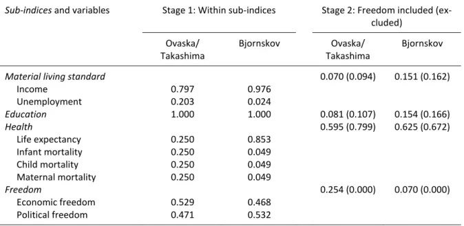
It can be seen, for example, that both studies give a comparably large weight to life expectancy – similar to Tofallis’s ap- proach mentioned above – but with regard to the other weights, which together still account for about one third, there are differences. On the basis of the initial weights thus determined for the individual variables, the weights to be applied in practice at the first stage of the weighted mean – i.e. within the sub-indices – and at the second stage (mean of the sub- indices themselves) were determined in a fourth step; the corresponding weights are shown

17

In the case of weighting scheme 1, for example, the following equation was solved according to x - the

weight of per capita income: 1 = x + 0.25x + 10.69x + 1.44x + 2.41x +2.15x.

20 in Table 6. In the following I will simply refer to weighting scheme one (Ovaska/Takashima data) and weighting scheme two (Bjørnskov et al. data).

Table 6: Weights applied on the first and second stages of the mean

Sub-indices and variables

Stage 1: Within sub-indices Stage 2: Freedom included (ex- cluded)

Ovaska/

Takashima

Bjornskov Ovaska/

Takashima

Bjornskov

Material living standard

0.070 (0.094) 0.151 (0.162)

Income 0.797 0.976

Unemployment 0.203 0.024

Education

1.000 1.000 0.081 (0.107) 0.154 (0.166)

Health

0.595 (0.799) 0.625 (0.672)

Life expectancy 0.250 0.853

Infant mortality 0.250 0.049

Child mortality 0.250 0.049

Maternal mortality 0.250 0.049

Freedom

0.254 (0.000) 0.070 (0.000)

Economic freedom 0.529 0.468

Political freedom 0.471 0.532

Sources: See Table 5; author’s own calculations.

A critical aspect of this approach certainly is the implicit basic assumption that the findings of happiness economics can easily be applied to the past. It is by no means clear that peo- ple’s life satisfaction at the time of the Weimar Republic, the Third Reich and the early Fed- eral Republic was determined by the same macroeconomic variables that determine life sat- isfaction in today’s societies. And even if there were reason to assume that the same deter- minants were at work, people at that time could at least have attributed different subjective weights to them – which brings us back to the point that no subjective survey data on pref- erences at that time is available (see the Wagner quote in Section I). The procedure chosen here can be checked for plausibility by reference to Wahl (2013: 97). In his study on living standards in the Third Reich he pointed out that among the countries examined in happiness economic studies there are usually those for which it holds that the level of development measured by per capita income and other variables is comparable with that of Germany in

18

Life expectancy’s large weight could be interpreted as a strong preference for health, which is specific to

highly developed societies, once more basic needs – e.g. for decent material well-being – are met. The level

of development of the social insurance and especially the health care system would presumably be an im-

portant determinant. There is no doubt that the German social insurance system before 1960, and especially

before 1945, was of a different quality.

21 the interwar period. In this respect, it is not unreasonable to assume stable and comparable preferences in the long term.

4. Discussing the variants of the Germany-specific Development Index

4.1. Influence of the mean concept on the construction of the standard of living

How much does our picture of the development of the standard of living in Germany change in comparison to Wagner’s estimation, if the geometric mean is used instead of the arithme- tic mean, but with the same data? A first look at Figure 3 immediately shows that the picture of a monotonically rising standard of living does not change after 1948, if one disregards the fact that the geometrically averaged DDI – subsequently abbreviated as DDI

– grows somewhat faster on average.

The case is quite different when looking at the interwar peri- od. First, the mere fact that the DDI

is lower than the DDI

does not per se indicate a lower level of prosperity. In formal terms, for any given year the difference itself merely in- dicates that the index values are scattered (see Section 3.1). However, meaningful state- ments can be derived from the change in the difference over time, and thus from the fluctu- ation pattern of the DDI

. Thus, the following deviations can be recorded: First, the level of prosperity rises only marginally from the local minimum in 1923 to 1924 (from 0.424 to 0.427 or by 0.7 percent compared to 3.6 percent for the DDI

). Second, the DDI

falls in 1926 to a level even below the initial level of 1920 (0.407 compared to 0.415), so that 1926 marks the absolute minimum in prosperity in the entire interwar period (according to the DDI

, this is 1920); compared to the DDI

, the increased unemployment here reflects much more clearly the stabilization crisis of the early “Golden Twenties” as well as the mini- mum in university participation.

Third, according to the DDI

, prosperity grows more strongly after 1926 and also until 1931, not 1930 (2.2 versus 0.7 percent p.a. over 1926-1930 and 2.7 versus 0.8 percent p.a. over 1926-1931); the DDI

also shows no dent in 1929.

Fourth, between 1931, the Weimar prosperity maximum (0.466), and 1936 prosperity falls steadily and significantly (by 2.3 per cent p.a.) to a level that corresponds at best to the

19

Between 1949 and 1960, the DDI

increases by an average of 1.68 percent and the DDI

by 2.15 percent.

20

According to Wagner’s data, the unemployment rate jumped from 3.4 % in 1925 to 10 % in 1926. For the

unemployment sub-index, this means a decline from 0.966 to 0.900 and for the combined sub-index of ma-

terial prosperity (plus per capita income) a decline from 0.765 to 0.733. In addition, the education sub-index

fell from 0.180 in 1924 to 0.150 in 1925 and in 1926, the minimum in the Weimar Republic.

22 worst years of the Weimar Republic – 1920, 1925 and 1926. The year 1936, i.e. the end of the first phase of the National Socialist regime, when full employment was achieved, turns out to be the actual minimum in the development of prosperity during the pre-war phase of the Third Reich, and not 1933 as suggested by the DDI

. Fifth, the DDI

implies a stronger and apparently catching-up growth in prosperity after 1936 until 1939 (4.6 percent p.a. ver- sus 2.6 percent p.a. based on the DDI

), the absolute maximum level of prosperity (0.474) in the interwar period; however, the increase in prosperity beyond the level finally achieved in the Weimar Republic, at 0.008 index points, is more than moderate compared to what the DDI

states (1930: 0.522; 1939: 0.565).

Sixth, finally, the prosperity gap is greater be- tween 1939 and 1949 when considering the DDI

.

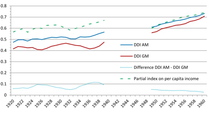
Figure 3: Classic DDI – arithmetic versus geometric mean

Notes: Indices equally weighted; no freedom index included.

Sources: See Figure 1, Table 1 and Table A.1; author’s own calculations.

From the temporal development of the difference between DDI

and DDI

(see the series at the bottom edge in Fig. 3), an interesting periodization of the interwar period follows:

Two phases can be identified in which the sub-indices per capita income, education and health grow in an increasingly balanced manner – i.e. the dispersion between the dimen- sions decreases –, namely between 1926 and 1932 and between 1938 and 1939. In contrast,

21

Note that the correlation between the two series (1920-1939), measured by Pearson’s correlation coeffi- cient, is moderately positive at 0.49. Moreover, the DDI

is growing by 0.9 percent p.a. overall over the in- terwar period, while the DDI

is growing by 0.7 percent p.a.

0 0.1 0.2 0.3 0.4 0.5 0.6 0.7 0.8

DDI AM DDI GM

Difference DDI AM - DDI GM

Partial index on per capita income

23 an increasingly unbalanced development of prosperity characterizes the phases 1920 to 1925 (ignoring the 1922/23 kink) and 1933 to 1937. The DDI

makes the deformation of the National Socialist economic miracle immediately apparent. In comparison to Wagner’s DDI,

“the DDI

[the author] does [not; the author] attest that the National Socialists significantly increased the prosperity of the German population compared to Weimar.”

The comparison of standardized per capita income with the DDI

, as shown in Figure 3, shows that it is very important for the assessment of the development of prosperity in the interwar period whether one relies on the DDI

or the DDI

favored here. Spoerer and Streb (2013: 137) engaged in the analogous graphical comparison of the sub-index per capita income with Wagner’s DDI. This comparison is important insofar as the fundamental criti- cism of the HDI is also grounded in the observation of a high positive correlation of the HDI with per capita income. And indeed, the correlation between per-capita income and the DDI

is highly positive at 0.93 (1949-1960: 0.99; 1920-1960: 0.90) in the period 1920 to 1939, so that one may get the impression that the information content of the DDI as an al- ternative measure of propserity is more than limited. Here, too, the picture for the interwar period is significantly different if the DDI

is used. It is striking that the marked slump in economic activity in 1923 is not reflected in the DDI

in the same way, but in the DDI

(see Figure 3). On the other hand, per capita income and the DDI

largely follow opposite paths, for instance from 1922 to 1923, 1925 to 1926 and especially 1930 to 1936. It is therefore not surprising that Pearson’s correlation coefficient of the two series is only 0.25, suggesting a merely weakly positive correlation. For the post-war period (0.98) and the period 1920 to 1960 as a whole (0.83), however, we can still speak of a high positive correlation.

According to DDI

, was the overall level of prosperity lower or higher compared to Wagner's DDI

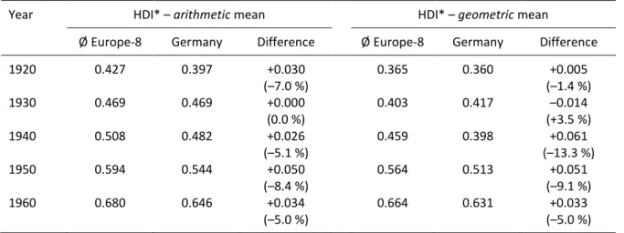
? This question can only be answered meaningfully within the framework of an international comparison. Such a comparison is possible on the basis of Table 7. For both mean value concepts the average HDI* (see Section 2) for the eight European comparison countries is shown using Wagner’s approach; the absolute and the percentage difference of the HDI* for Germany to the European average is shown.

Reviewing the arithmetically averaged HDI*, the level of prosperity in the Weimar Re- public around 1920 is initially below the European average. This shortfall is completely made

22

Here, the modified assessment of Spoerer/Streb (2013: 137) on the DDI

.