RESH Discussion Papers
No. 3 / 2020
Tobias A. Jopp/Mark Spoerer
Teaching Historical Statistics: Source-Critical Mediation of Aims and Methods of Statistical Approaches in History
FAKULTÄT FÜR PHILOSOPHIE, KUNST-, GESCHICHTS- UND GESELLSCHAFTSWISSENSCHAFTEN
i
REGENSBURG ECONOMIC AND SOCIAL HISTORY (RESH) Discussion Paper Series
Edited by
Prof. Dr. Mark Spoerer and Dr. Tobias A. Jopp
Processed by Dr. Tobias A. Jopp
University of Regensburg
Faculty of Philosophy, Art History, History and Humanities Department of History
Chair for Economic and Social History
The RESH Papers are intended to provide economic and social historians and other historians or economists at the University of Regensburg whose work is sufficiently intersecting with economic and social history with the possibility to circulate their work in an informal, easy-to-access way among the academic community. Econo- mic and social historians from outside the University of Regensburg may also consider the RESH Papers as a means to publish informally as long as their work meets the academic standards of the discipline. Publishable in the RESH Papers is the following: Work in progress on which the author(s) wish to generate comments by their peers before formally publishing it in an academic journal or book; and English translations of already published, yet non-English works that may be of interest beyond the originally targeted (German, French, and so on) audience.
Authors interested in publishing in the RESH Papers may contact one of the editors (Mark.Spoerer@ ur.de; Tobias.Jopp@ur.de).
Cover page photo on the left: Real GDP per capita for selected regions in the long term. Source: Figure produced from the Maddison-database available at: https://www.rug.nl/ggdc/historical-development/maddison/releases/ maddison-project- database-2018 as updated and described by Bolt et al. (2018); accessed: 3 May 2019.
Final page photos: Own material.
ii
Teaching Historical Statistics: Source-Critical Mediation of Aims and Methods of Statistical Approaches in Historiography
Tobias A. Jopp / Mark Spoerer
Abstract: This monograph helps historians design a low-threshold introductory course on historical statistics. The course aims at providing students with elementary knowledge enabling them to understand historical studies that apply statistical methods. Elementary is meant to include the tools of descriptive statistics and correlation analysis in the first place. We develop the course along these core themes: Objective and target groups; statistical reasoning; basic knowledge; pitfalls; the typical quantifying research approach; and course design.
Keywords: Historical statistics, teaching JEL classification: C00, N01
This discussion paper is a translation of a short monograph originally written in German. Possible revisions to the original version (inclusion of new literature and/or new evidence) are indicated as such. The original publication is: Tobias A. Jopp/Mark Spoerer (2017): Historische Statistik lehren. Quellenkritische Vermittlung von Zielen und Methoden statistischen Arbeitens in der Geschichtswissenschaft. Please cite the original publication along with this discussion paper.
Contact 1: Dr. Tobias A. Jopp, University of Regensburg, Department of History, Economic and Social History,
93040 Regensburg; email: Tobias.Jopp@ur.de. Contact 2: Prof. Dr. Mark Spoerer, University of Regensburg,
Department of History, Economic and Social History, 93040 Regensburg; email: Mark.Spoerer@ur.de.
1
Teaching Historical Statistics: Source-Critical Mediation of Aims and Methods of Statistical Approaches in Historiography
1. Introduction
"More", "less", "some" etcetera – historiographic narratives are plentiful with indefinite numerical words indicating an implicit numerical comparison of two sets. In many cases (such a word, too!) only such comparisons allow placing a certain set of facts in one’s argument. Often(!) author and reader are satisfied with such a rather vague comparison. But sentences like "Many newborns died soon after birth" will leave some(!) readers somewhat(!) perplexed: how long is "soon after birth"? And what does "many" mean in the context of a time period when only, say, 3.2 per thousand (i.e. three out of a thousand) of the babies born alive die in the first twelve months after birth? Ten percent? A quarter?
Half? Or even more? Many readers would certainly prefer a more precise statement, such as
"36.4 percent of babies born alive died within the first twelve months after birth in 1853".
But more critical readers would subject this statement to a thorough review of sources and methods: is the source reliable? Is 1853 a normal year or an outlier? Which factors may distort the result (e.g. practice of making entries in the church register)? And, in general, does not the saying apply which is (very probably wrongly) attributed to Winston Churchill:
"The only statistics you can trust are those you falsified yourself" (Barke 2011: 7, 11)?
Statistics for historians?
Is it possible to work seriously with statistics as a source- and method-critical historian, at all? In our opinion, it is indeed; and this is precisely why we have written this introduction. It is true that numbers-intensive historical studies sometimes leave a bland aftertaste in the minds of readers who are inexperienced as regards statistics. This is especially true if such studies do not remain on the level of description, but investigate cause-effect relationships mathematically or in terms of probability theory. Of course, every source must be critically scrutinized, especially since statistical data are not collected just like that, but always for a specific purpose – but this applies to almost all sources. The choice of statistical tools, i.e.
the methodology, must also be made comprehensible to informed readers. If sceptics
continue to categorically reject the methods of historical statistics, we think two things are
at work: ignorance and resentment (Kaelble 1990; Jarausch 1990). With this guide we can
2 counter the former to a certain extent and hopefully alleviate the latter at least somewhat.
Two examples will illustrate the potential of historical statistics.
Two examples
How many "witches" were actually burned in Europe? And who was the typical voter of the NSDAP who helped it to achieve the high election results of 1932 and 1933? These are just two (arbitrarily selected) questions out of a whole series of important questions that have been occupying historical research for a long time and for which it is hardly possible to find answers without the collection and analysis of statistical data.
Nine million witches?
In the first case, historians have devoted themselves to the deconstruction of the "myth of the nine million witches" executed in total – a persistent myth that originated in the late 18th century and has been regularly re-fed for political purposes ever since. Today, on the basis of thorough research that allows plausible estimates, a number of witch executions in the order of 30,000-50,000 seems much more likely (Behringer 1998: 683).
The typical National Socialist voter?
In the second case, historical electoral research has advanced the "demystifying of 'electoral historical folklore' about National Socialism" (Falter 1979: 3) and fundamentally revised our idea of the profile of the typical NSDAP voter. Contrary to an opinion that had prevailed for decades, "[...] the NSDAP [succeeded] in mobilizing members of all social strata in such large numbers that, despite the overrepresentation of the Protestant middle class, it had a more popular party character than any other political grouping of those years" (Falter 1979: 19).
These examples suggest that it is also worthwhile for a historian to have statistical knowledge; be it in order to pursue certain research questions herself, or simply to be able to critically read and understand relevant studies.
This book’s objective
This book is primarily intended to help historians teaching at universities to design a low-
threshold course on historical statistics. It is intended to provide students with elementary
knowledge for a better understanding of historical studies that use statistical methods. With
3 the exception of the sub-discipline "economic history" – the sub-discipline that relies most heavily on statistics and especially inferential statistics for the analysis of cause-and-effect relationships – "elementary knowledge" primarily includes knowledge of the tools of descriptive statistics, with which the central characteristics of an existing data set can be worked out, and of correlation analysis.
In addition to the question of what content a basic course should cover (Chapter 4), we also provide you as a lecturer with arguments that help convince students of the usefulness of a course on historical statistics (Chapter 3). However, we like to start by placing the term.
2. Definitions
Statistics
"Statistics" refers to "[...] a science that provides methods for extracting data and learning from data". Irrespective of the concrete field of application, statistics essentially is always based on the same work steps, namely the "collection of data", the "description and visualisation of the collected data", the "identification of anomalies in the data" and the
"derivation of conclusions that clearly go beyond the available data" (Mittag 2016: 7). Apart from referring to a science with its special canon of methods, the term "statistics" also refers to a self-created, mostly tabulated dataset, an official or semi-official data compilation, or a parameter derived from the data (e.g. a mean value).
Historical statistics
But what is "historical statistics"? Is there content specifically tailored to historiography that
distinguishes historical statistics from statistics in general or economic statistics, medical
statistics, etcetera? Or does the addition merely imply that identical content is conveyed in
the best language for the respective discipline? There is no doubt that formula language and
jargon are significantly downscaled in relevant introductions (Hudson/Ishizu 2017). Apart
from this aspect, however, a distinguishing feature of historical statistics precisely is the fact
that greater importance must be attached to the step of "collecting data", quite simply in
order to take into account the nature and contextuality of historical sources for statistical
data (Tilly 1976: 48). The training of historians should therefore also raise awareness of the
special sources of historical statistics. However, despite the fact that computer software is
4 now very powerful, there is no such thing as a standardised procedure in historical statistics;
each question requires an individual approach.
In addition to the term "historical statistics", other terms with similar meanings are in use, such as "quantitative methods in historiography", "quantitative history", "quantification in historiography" and "cliometrics" (for another term – "historical social research" – cf. e.g.
Schröder 1994). Basically, Jürgen Kocka's definition of "quantification" can be understood equally as a definition of all other terms; in his words: "Quantification in historiography – that means the systematic processing of identical source information (or data) that can be numerically summarized with the help of diverse arithmetic and statistical methods for the purpose of describing and analysing historical reality" (Kocka 1977: 4; similar Jarausch 1976:
12).
Cliometrics
The term "cliometrics" – a combination of "clio", the muse of historiography, and the suffix
"-metry" for "measurement" – requires a separate explanation. Even if the relevant Duden entry – cliometrics is the "development of historical sources with the help of quantifying methods" (retrieved at www.duden.de/suchen/dudenonline/cliometrics; 4 Aug 2016, 16:55h) – makes sense literally, the term is specifically connoted in the relevant literature with economic history, which draws on social science methods, and is sometimes equated with "econometrics", which stands for quantitative methods in the economic sciences. In this sense, working cliometrically means in particular "[...] the formulation of working hypotheses through the explicit use of theoretical models (mostly from economics, but also from other disciplines such as sociology, demography or biology)" (Komlos/Eddie 1999: 20).
In the following we use the adjectives "statistical" and "quantitative" synonymously.
When we speak of "historical statistics", we mean the toolbox – that is, the sum of all
relevant statistical methods including the possibilities of source criticism. In this sense, we
also use the formulations "historical statistics", "cliometrics", "quantification in
historiography" and "statistical work in historiography" synonymously.
5 3. Historiography and statistics
3.1 Statistical sources
Critical source analysis is the basis of the historian’s work. It is common practice to divide sources into real relics, and oral and written testimonies that directly or indirectly represent a historical phenomenon. Of particular importance as basis for a quantitative analysis are written, mostly non-narrative testimonies (for a counter-example, cf. "quantitative vs.
qualitative sources"), and among these the "legal sources" and the "administrative documents" ("social documents") (Howell/Prevenier 2004: 24-26).
Historical statistics presupposes the existence of masses of uniform observations. An observation exists when, for a unit of investigation (the "feature carrier"; e.g. a country; cf.
below), a certain amount of information (a "feature"; e.g. the number of infants that died in 1853 per thousand live births) is gathered by determining a numerical value (the "feature value"; e.g. 10 per 1,000). A single unit of investigation with the information gathered on that unit constitutes a case. Each specific piece of information is considered a variable, and the total number of cases constitutes the dataset (Hudson/Ishizu 2017: 50).
Case no. Observational unit Point in time of observation Mortality …
1 Prussia 1853 44 …
2 Bavaria 1853 42 …
3 Prussia 1863 42 …
4 Bavaria 1863 45 …
… … … … …
Types of datasets
In general, three types of data records can be distinguished:
– Cross-sectional dataset: infant mortality is collected for a uniform period in different regions, i.e. observations are only collected across space (cases 1 and 2).
– Longitudinal dataset: infant mortality is collected for a uniform region over a certain period of time with several sub-periods (monthly, annually, 5 years), i.e. observations only are collected across time (cases 1 and 3).
– Panel dataset: infant mortality in different regions and over a certain period of time with
several sub-periods is collected, i.e. the observations are collected across space and time
(cases 1 to 4) (Note that while in the classical panel the cross-sectional dimension is larger
6 than the time dimension, the time series cross-section has few units of investigation which, however, have been recorded for a very large number of points in time; Feinstein/Thomas 2002: 8-9).
Types of sources
In addition, four types of statistical sources can be distinguished, the first three of which have a time component, either directly or by combining one another:
Type 1 (serial source in the sense of the term): a type of source that has been deliberately designed by the author (authorities, church, private institution) as continuous and (more or less) standardised in its appearance (e.g. publications of official statistics; church books/ac- counting books).
Type 2 (serial source in the broadest sense): one that was not consciously created as part of a series, but was nevertheless produced regularly in a (more or less) standardised form (e.g.
wills). The series only emerges from the historian's perspective when linking comparable documents to a dataset.
Type 3 (quasi-serial source): one that is basically non-serial, i.e. that has not been consciously designed as continuous and not standardised in appearance, but which could also serve as a starting point for the historian to work out a series; this could, for example, be a dissertation from a certain academic discipline which is examined as to see whether its formal composition has been subject to changes over time.
Type 4 (non-serial source): A source that only contains data at a specific point in time (keyword "cross-sectional data set").
Whether a source can be described as a serial source of type 2 or 3 depends very much on the historian's concrete epistemological interest or, respectively, the specific question posed, i.e. ultimately on the individual case.
Quantitative versus qualitative sources
Statistical sources can be both quantitative and qualitative sources, i.e. they can report rather numerical (e.g. statistics of the German Reich) or rather non-numerical news (e.g.
birth certificate). The former often occur in the form of lists, tables, or figures, but
sometimes also as continuous text. If a table is available, this makes the data gathering
easier in principle; if necessary, one simply records a value taken from a table and repeats
7 this process year-by-year, for example. In comparison, the extraction of observations from qualitative sources involves considerably more effort, especially with regard to classification, categorisation and coding – i.e., the translation of qualitative information into a numerical value. A good example of this "translation service" is provided by Morris (1999), who, among other things, examines the social structure of the British middle class on the basis of the parliamentary poll books of the city of Leeds for the year 1832. Before the introduction of the secret ballot, the poll books explicitly noted for which candidate an eligible voter, recorded by name and profession, voted. Similarly, Kruedener (1975) and Grabas (2011) carried out qualitative economic analyses based on "narrative" annual reports from the Preußische Bank, on the one hand, and the Saarbrücken Chamber of Commerce, on the other. Likewise innovative is the volume by Aly (2006) on the measurement of public opinion in the Third Reich (On the development of archives, official statistics and statistical thinking – important topics that we will leave out in the following, however –, cf. e.g. Pitz 1976;
Schneider 2013; and Reininghaus 2014).
Source criticism on statistical sources
No source that has come down to us, whether it is textual or statistical, has been designed specifically for the purposes of the historian in the future. In order to work out, on the one hand, the view of the source's author on the historical reality which he or she witnessed and, on the other hand, the author’s agenda, a critical analysis of the source is necessary (cf. for the common principles Howell/Prevenier 2004: 76-78). For the historian trained in the criticism of qualitative, textual sources, the criticism of quantitative sources will certainly be unusual. How does one criticize a source that reports a lot of numbers?
First of all, by asking certain questions about the source that one would ask about any other source in a similar way: who exactly is the author? Out of which interest, for what purpose and how were the raw data originally collected? What categorisation schemes or demarcations were once used to condense the raw data and the information contained therein? Which information was lost or deliberately "destroyed" in the course of the aggregation process? Which "administrative will" can be reconstructed from the source?
Ultimately, and this is what makes source criticism so difficult, the questions that one should
ask depend very much on the nature of the source and the quantitative data reported there,
but also on the questions one wants to ask oneself (Tilly 1976: 46; de Vries 1980: 434; and
8 Hudson/Ishizu 2017: 13-15). It is crucial that the historian gets an idea of the context in which the source was created.
Gaining information by losing information
The goal of source criticism must be to assess the selectivity of the statistical information conveyed as it is initially available to the historian. This is the basis for the following steps – data selection and further processing – and also the basic prerequisite for assessing the representativeness of the constructed dataset. The historian should always be aware of the tension inherent in quantitative work between information gain, on the one hand, and information loss, on the other. More pointedly: in the course of identifying, categorising, classifying, and coding news, information must inevitably get lost in order to open up new perspectives on the object of research. The historian certainly has a greater influence on this loss of information when she begins to construct a dataset from a qualitative source than when she uses statistics that are themselves the result of processing on the part of the source’s author (cf. for some examples Rohlinger 1982: 43).
Representativeness
One example may help: Referring to the US, Sharpless and Shortridge (1975) and Conk (1981) discuss the general weaknesses of census data and occupation censuses of the 19th and 20th centuries. Distortions result, among other things, from the fact that "never all the people who should actually be counted are counted", which may be related to the fact that respondents answer incorrectly or the capacities of the census authorities to conduct thorough and comprehensive surveys are insufficient. This underestimation can be particularly problematic if it occurs systematically (due to institutional racism or a change in the coding scheme, for example) because this means that certain groups of individuals are non-randomly wrongly described or under- or over-represented. Other interesting examples are discussed by Tilly (1976) and De Vries (1980).
Source criticism using statistical methods
Criticism of one's own quantitative sources can also rely on statistical methods. A good
example from the field of population statistics is the phenomenon of the so-called digit
preference: people may not report their age correctly, for example when they are
9 interviewed in a population census. Perhaps, this is rooted in cultural or religious beliefs;
perhaps, respondents simply do not know their true age. As a result, single-year-of-age data, and analytical tools based on them such as the population pyramid, may be biased in that some ages are extremely common and others are under-reported. For example, there is a common preference for ages ending in 0 and 5, and their clustering is seen as a sign of low educational attainment in a population. An example of cultural/religious numerical preference in East Asia is the accumulation of ages ending in 3 and the insufficient occurrence of those ending in 4. These distortions may also be present in historical population data. In order to determine their extent, historians can calculate the so-called Whipple index and similar indices – statistical measures that determine the quality of the data based on the distribution of reported individual ages (Poston 2005: 25, 34-36;
Tollnek/Baten 2016).
A further example comes from the numerous approaches of anthropometric history dealing with the analysis of body height in a community in order to derive statements about the so-called biological standard of living. Traditionally, conclusions about the living standard of a population are mainly drawn on the basis of the heights of soldiers (partly also of prisoners). Statistical methods illustrate that the recording of heights was subject to certain rules (e.g. minimum height for conscripts) which can distort a data set and reduce its representativeness (Bodenhorn et al. 2017).
3.2 Potentials and limits
In addition to the availability of a set of similar observations, further prerequisites must be met in order to use historical statistics profitably: the phenomenon to be explained must be intrinsically quantifiable and variance in the data must be relevant for the argumentation.
Moreover, the higher the number of cases considered and the more complex the chosen explanatory approach, the more worthwhile quantification is (Tilly 1987: 22; and Jarausch 1976: 14). We want to address these points by first naming the arguments usually put forward against quantification and then briefly turning to its advantages or, respectively, potential (Jarausch 1976: 15-16; Stone 1979; Clubb 1980; Aydelotte 1984; Botz 1984: 58-60;
Monkkonen 1984: 90-91; Kaelble 1990: 76-78; Schröder 1994: 8-9; Sewell 2005: 6-8;
Hudson/Ishizu 2017: 1-3):
10 Contra quantification
1a. Non-descriptive language: the formal language of quantification does not match the style in the humanities and the linguistic diversity of expression that a good historian’s narrative should be showing.
2a. Illusion of precision: the use of numbers suggests a precision or certainty in the description and explanation of historical phenomena which is inappropriate. By generating statistical data and analysing them, the historian creates a distorted and/or incomplete picture of historical reality.
3a. Lack of representativeness: since the collection of data in the past was the result of interest-led action, its evaluation by historians will only in exceptional cases really provide a representative picture.
4a. Non-historical results: the results of statistical analysis are established ex post and were not available to contemporaries; therefore they cannot have influenced their actions.
5a. Methodological fetishism: quantitative works regularly get lost in mathematical- statistical questions of detail; the fine-tuning of models and calculation methods only obscures the view of the "number juggler" as well as the reader for the historical context and the historical phenomenon that actually needs explaining.
6a. Quantification promotes a change in research strategy – not to say in researcher mentality: instead of addressing the big, important questions of history – no matter how laborious finding answer might be – the quantifier picks out the objects and questions of research that can be statistically assessed; often the dataset, which was collected just because it could be collected, is established first, and only then is the research question matched to it.
7a. Trivial findings: the results to be obtained by quantification do not justify the necessary effort since they have no (significant) surplus value beyond findings obtained on the basis of the classical, historical-hermeneutic method.
8a. No sense of historical singularity/wrong understanding of time: quantifiers underestimate or even ignore the historical events’ "boundedness in time and culture"
(Jarausch 1976: 15) and thus their uniqueness; this makes the assumption of time-invariant
regularities appear absurd and thus sets limits to any attempt at generalisation. If a historian
11 works quantitatively, she inevitably adopts a false understanding of the "temporalities of social life" (Sewell 2005: 6).
Pro quantification
1b. Standardized modus communicandi: quantification in the form of formulas, tables, and graphs is a standardized, effective way of gaining and illustrating knowledge that facilitates expert discussion. Being able to follow this path also enables the historian to engage in interdisciplinary dialogue with the social sciences.
2b. Genre-specific analysis tool/analysis of mass phenomena: quantification is a suitable method for processing the many existing serial sources and the data to be obtained from them. This inevitably comes with a focus on structural relationships and groups of individuals belonging to the anonymous mass of ordinary people; both provide the basis for an average view, which is the main focus of quantitative work.
3b. Universalization: the nature of the sources corresponds to the fact that (usually) it is not a particular unit of investigation with its particularities – a certain individual or a certain entity from a set of individuals or entities – that is of interest, but rather the commonalities connecting all units of investigation, the accumulation of which can only be assessed through statistical analysis ("group characteristics"; Jarausch 1976: 16). Only the description of a historical phenomenon using statistical data can improve our level of knowledge. In addition, quantification can serve to test theoretical, social science-based statements about human or group behaviour and to uncover behavioural laws (influence of framework conditions) or identify deviations in need of an explanation (proximity to the nomothetic understanding of knowledge). This requires variance in the data – in other words: a diversity of (groups of) individuals reflected in the sources.
4b. Special form of comparison: considering the fact that in historical narratives implicit numerical comparisons occur regularly, quantification merely is a form of comparison in which the quantities to be compared are made explicitly visible.
5b. Analysis of "natural experiments": the essence of (natural) scientific work is "the controlled and repeatable experiment" which is used to "establish chains of cause and effect" by isolating the crucial variables. Such experiments are understandably not possible when dealing with the past. An approximate solution to this problem is the so-called
"natural experiment": "One searches for and finds natural situations that differ in the one
12 variable whose influence one seeks to determine". Provided that the historian "finds" such a situation, historical statistics are a helpful tool for its analysis (Diamond/Robinson 2010: 1-2).
Pragmatic plea
What is our conclusion of the debate about the sense and nonsense of quantification? To put the criticisms two and three into perspective, one might object that the same can be said about the use of qualitative methods. Nevertheless, the question of the representativeness or precision of statistical data is central to historical statistics so that the criticism is justified in any case. We will therefore go into this point in detail later. Whether it is necessary to calculate many models or whether the results are really trivial is, in our opinion, primarily a question of communication.
We believe that two things are crucial: firstly, to be able to acknowledge that there are types of historical sources which, because of their internal structure and the nature of the messages contained in them, can only be meaningfully evaluated by using quantitative methods. And even if the application of qualitative methods alone already provides valuable insights, quantitative methods open up additional perspectives that qualitative methods simply cannot. It is true that recourse to quantitative methods inevitably entails a change of perspective – away from single prominent individuals and historical singularities and towards structures and frameworks within which statesmen and thinkers as well as the innumerable nameless members of a society acted and possibly showed recurring (behavioral) patterns.
Secondly, any historical phenomenon has to be dealt with in a reasonable way; if possible all available sources – i.e. quantifiable as well as non-quantifiable sources – have to be analyzed in combination (cf. Carus/Ogilvie 2009). Qualitative and quantitative historical methods are not mutually exclusive, but ideally complement and stimulate each other.
3.3 The history of quantification in historiography
Following the abstract discussion of the pros and cons, we now want to outline how quantitative methods entered into (German) historiography.
Historicism
In the long term, the movement of historicism in 19th and early 20th century Germany has
been the determining factor for the attitude of historians towards statistics. Following Kocka
13 (1975: 5), the historical-critical method, the core of this influential movement, aims at the
"hermeneutic interpretation" of the source material. According to the nature of the method, this interpretation rather is "literary-linguistic" and should provide information about the
"traditional motivations, attitudes and actions of the great actors", and not about the
"supra-individual structures and processes" as they become visible especially through the evaluation of quantitative sources. This notion by no means only dominated German historiography, but rather that of the 19th century in general. With their nation-state orientation, their representatives saw no reason to argue with statistical data when the major topics of interest were those of political and diplomatic history and the history of great ideas of individual historical figures.
The Historical School versus Marginalism
An important exception is connected with the Historical School of Economics: the methodological dispute between its representatives (such as Roscher, von Schmoller, and Wagner) and the followers of Marginalism – the abstract theorists around C. Menger – led to an empirical interest in the social environment for the first time in the last third of the 19th century. The preference of the followers of the Historical School of Economics for empirical, historical facts (and historical phase models for describing the history of humanity and its economic actions) brought them close to the historians, among whom above all Karl Lamprecht, under the influence of Roscher, called for an empirically saturated cultural history (Söllner 2001: 271-273). So inspired, historiographical works (also) based on numbers were written in the late 19th century (e.g. von Schmoller 1898).
Annales School
The Annales School in France provided a first and lasting impulse to quantification in the interwar period; its followers (such as Bloch, Febvre, Furet, later Braudel, and Le Roy Ladurie) turned away from the event- and person-oriented historiography that had hitherto dominated there, and focused their efforts on the identification of long-term structures and processes (longue durée and histoire totale) (Jarausch 1990: 49; Lengwiler 2011: 159).
Economic and socio-historical questions that focused on population, settlement, and
occupational or economic structures gained importance, and with them new objects or
collective phenomena – such as prices, the family, or mentality (Lengwiler 2011: 159). While
14 in a first phase (until about 1945) the followers of the Annales basically pursued "qualitative structural history", in a second phase (until about the beginning of the 1970s) they devoted themselves specifically to "quantitative economic history" (Labrousse et al. 1970; for the quotations Botz 1984: 55-56).
Pioneer North America
The United States can be considered a pioneer in terms of quantification in the strict sense.
Methodological advances in statistics after the Second World War led to an increasing number of authors of economic studies using inferential statistical (econometric) methods;
authors included those whose approaches were to found cliometrics (e.g. Robert W. Fogel).
However, methods of descriptive statistics also found their way into historiography itself in the 1950s and 1960s – as the core of "new social history" and "new political history", for example (Bogue 1981: 141; Jarausch 1990: 46-47). As part of the former, questions about the social stratification of societies and demographic developments were asked and groups of people were brought into the focus of historiography that were previously uninteresting;
as part of the latter, for example, systematic, data-based research into voter behaviour and the social structure of the electorate and political elites made its mark (e.g. Fogel 1975: 332- 333; Tilly 1987: 22-23; Sewell 2005: 26-27) (Note that new journals such as Comparative Studies in Society and History (1958), Journal of Social History (1967), Historical Methods Newsletter/Historical Methods: A Journal of Quantitative and Interdisciplinary History (1967), Journal of Interdisciplinary History (1970) and Social Science History (1976) bear witness to this change).
Adoption in Germany
In Germany, quantitative methods were applied much more hesitantly than in the Anglo-
Saxon world and France because the reservations against any attempts at quantification
were more deeply rooted. Taking the angle of the sociology of science, this was due to pride
in the historiographical tradition of the profession, but also to the conviction that the
complexity and time-bound nature of historical reality was not suitable for a quantifying
access, especially since the data basis was inadequate due to poor tradition, and thus a
glaring disproportion between costs and benefits was to be expected (Kocka 1977: 7-9).
15 Historical social sciences
Quantitative methods did not make a lasting impact on German historical scholarship until the first half of the 1970s with the emergence of historical social science, which is closely linked to the Bielefeld School centring on its founders Hans-Ulrich Wehler and Jürgen Kocka, as well as with the founding of the Centre for Historical Social Research at the University of Cologne and the establishment of the working group for quantification and methods in historical social science research, QUANTUM (Jarausch 1976: 24; Iggers 2007: 32-34). History and Society (since 1975) and Historical Social Research (since 1976, initially under the title QUANTUM Information) were advanced and became the two most important publication organs of a social science and quantitatively informed historiography. As before in the United States, and with a stronger theoretical orientation than, for example, in France, the focus of research shifted to social or societal history with its interest in groups of (anonymous) individuals and in the persistence or even mutability of supra-individual social structures (cf. Jarausch 1976: 19ff; Jarausch 1990: 50). In the context of political history, research into public opinion and political voting behaviour has been promoted by the use of social science methods (cf. Jarausch 1976: 17-19; Falter 2015; for thematic focuses Oberwittler 1993: 91).
Cultural turn
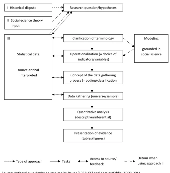
The "cultural turn" of the late 1980s, which relied on "dense description" and the supporters of which were not interested in quantification (cf. Iggers 2007: 61-62), presumably stopped a further diffusion of the application of quantitative methods on a broad scale. If all tables and graphs of statistical data published in Geschichte und Gesellschaft since 1975 are counted, the following picture emerges that is entirely consistent with this assessment (cf. Figure 1):
The frequency of both tables and figures per 100 pages was meanwhile six or just over two,
respectively, and has declined in the long term. This can probably be explained by a change
in the range of topics and methods as a result of the culturalist and linguistic turnaround.
16 Figure 1: Tables and graphs per 100 pages in Geschichte und Gesellschaft
Notes: Depicted is a three-year centred moving average.
Source: Own presentation based on a total survey of the journal Geschichte und Gesellschaft in the period 1975-2016 (research articles plus discussion forum).
In our opinion, however, many historians' fears of "statistics" have eased in recent years.
Contemporary historians, in particular, are increasingly working with social statistical data that can be used to illustrate phenomena such as the change in social values (cf. Dietz et al.
2014; Raphael/Wagner 2015). A very important point here is the much simpler processing of data today by standard computer programs.
4. Planning and implementation of a course
Hopefully, we were able to make clear that quantification can in principle contribute to the progress of knowledge in historiography, but that this potential has so far been insufficiently exploited. In order to prevent the existing relevant approaches from sooner or later disappearing in the Bermuda Triangle of historiography or, at best, from being noticed in very specialized discourses among researchers themselves, historians' education should also include training in reading comprehension and judgment in the field of statistical analysis. In this section, we want to provide assistance in defining the learning goals and teaching content of a basic course starting at this point. We assume that attending the course will be on a voluntary basis, which is why the participants will be sufficiently motivated to work on historical statistics – also and especially because they can see the value added for their further studies and professional life (cf. Best/Schröder 1981; Schuler 1981).
0 1 2 3 4 5 6 7
Tabellen pro 100 Seiten Abbildungen pro 100 Seiten
Tables per 100 pages
Graphs per 100 pages
17 4.1 Objectives and groups
Course’s objective
A course following our proposal has two primary objectives: on the one hand, to transform a rather diffuse initial student interest in historical statistics into a concrete idea of its possible applications; and, on the other hand, to encourage the participants' willingness to continue their education in this field independently, if necessary. At the end of the course, students should at least be able to (better) assess the value of quantifying studies and to refer to those studies’ results in their own work; in the best case, they should even feel inspired to carry out a quantitative analysis in the context of a seminar or qualification thesis.
Reading to comprehend
In our opinion, these primary course objectives can be achieved by providing participants with the basic knowledge for "reading to comprehend" quantitative work on a practical level, so that they can answer the following questions to a typical study: what research question is the study going to answer? What is the author's methodological approach to answering it? Why this particular approach, and not a different one? What are the pitfalls of the chosen methodological approach in connection with the source base? Are the results illustrated and interpreted in a comprehensible way, especially with regard to the question?
What are the consequences for our understanding of the historical phenomenon under consideration? In order to visualize this goal, relevant tables and graphs of varying degrees of difficulty could be presented to the students at the beginning of the course and discussed with regard to the supposedly correct reading (cf. for many examples Feinstein/Thomas 2002; Hudson/Ishizu 2017). The same materials (and possibly others to test the ability to transfer) could be used again as a basis for a final learning objectives check.
Preconditions and prior knowledge
Where should the addressees of this course stand in their studies of history? And what
previous knowledge should they have? In our opinion, an upper limit does not make sense,
but a lower limit is useful. The course should be addressed to all those who are already
somewhat trained in the application of the classical tools of the historian, i.e. the
hermeneutic and comprehensible interpretation of source material or, more generally
18 speaking, qualitative methods. In the normal course of studies, we think that fourth- and higher semesters are the appropriate addressees.
A word on the problematic subject of "mathematics": having a basic knowledge of mathematics is undoubtedly beneficial for successfully participating in this course. In fact, one only needs to have basic arithmetic knowledge, needs to know the rule of three and percentage calculation, and has to understand probability theory to be able to master a text such as Feinstein and Thomas (2002).
Two target groups – one approach?
Yes, this course is equally suitable for prospective history teachers as well as all other prospective historians – regardless of the occupation they are aiming for. Whenever dealing with historical source material, a basic knowledge of historical statistics can only be beneficial. In addition, general statistical knowledge can be used as a key competence in many areas of the economy – if it is not even part of the everyday knowledge of the responsible citizen, who to "raise" is also the task of history teaching. The didactic significance of statistics in school lessons should be explicitly addressed when student that become teachers participate (cf. Mayer 1999; Sauer 2007: 255-256).
4.2 Statistical thinking
Representativeness
Statistics is based on certain basic insights about its subject matter – insights which one
needs to get familiar with. To a certain extent, it is necessary to learn how to "think
statistically". In this section, we will briefly address the basic insights that seem most
important to us. They are as follows: the aim is to gain knowledge about the characteristics
of a basic population of interest (which is sometimes a challenge to define correctly; cf. de
Vries 1980: 437-438). However, this population cannot be grasped in its entirety, but only in
part. Conclusions about the characteristics of the population are to be drawn on the basis of
a section – the so-called sample. The conclusion on the population drawn from the sample is
subject to uncertainty because the statistical characteristics of the sample and the
population will generally not coincide. This raises the central question of representativeness
(of the sample for the population).
19 Sample and population
From this uncertainty the probabilistic foundations of statistics follow directly: it is possible that the characteristics of the sample and those of the population will coincide completely, only a little, or not at all. In short, there is an ex ante range of possibilities of how the sample will position itself vis-à-vis the population; formally speaking, this range represents a so- called (probability) distribution of characteristic values over all possible values. For an intuitive understanding, it is important to remember at this point that there are three distributions we should distinguish: firstly, the unknown distribution of the characteristic in the population (e.g. infant mortality in the Prussian communities in 1853); secondly, the distribution of that characteristic in the available sample (e.g. containing 10% of all Prussian communities); and, thirdly, the distribution of a key figure of interest – e.g. the sample mean value (cf. below) – over all possible samples to be drawn from the population. The first two distributions are empirical distributions that result from the data at hand (the distribution in the population cannot be observed, however); the latter is a theoretical distribution that follows certain formal considerations or, respectively, assumptions.
The fact that the latter distribution is a theoretical – one could also say: hypothetical – distribution follows from the basic insight that the population is not completely ascertainable: simply not all samples that would have to be collected for complete coverage can in fact be collected. Ultimately, statistical tools are designed to help answer the following question: how large is the probability that the statements derived from the present sample would have followed in exactly the same way from other samples? If a high probability can be expected, the present sample would be representative (cf.
Jarausch/Hardy 1991: 63-65; Feinstein/Thomas 2002: 117-119).
4.3 Basic knowledge
In this section, we will briefly discuss those statistical concepts that a basic course in historical statistics should definitely deal with (cf. also Section 4.6).
Classification of characteristics
We will start with a few obligatory remarks on the classification of characteristics. Their
properties determine which arithmetic operations are possible – i.e. which tools are
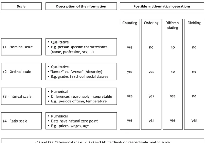
applicable – in the context of a statistical analysis. Figure 2 shows which properties are to be
20 distinguished in this sense. Formally, it is a matter of the data’s level of measurement; we can generally distinguish between four measurement levels, whereby the information content of the data increases with the transition from level (1) to level (4) because the range of applicable tools is widening. Basically, qualitative sources tend to yield categorical data, whereas quantitative sources yield primarily metrically scaled data.
A further classification of characteristics results if one asks for the range of expressions or numerical values that it can assume in principle (cf. Mittag 2016: 18-19): a so-called discrete characteristic can only assume a finite number of values; counting data, for example, are always discrete (e.g. the number of cars one owns or of babies who died in year x etcetera) – and also assume integer values. In contrast, a so-called continuous characteristic can, in principle, take on all conceivable values in an interval (such as age or prices). Continuous characteristics can easily be converted into discrete characteristics by creating classes or, respectively, groups to improve on visualizing them in graphs or tables.
Figure 2: Level of measurement of observations
Source: Authors' own depiction following Hudson/Ishizu (2017: 45-46) and Mittag (2016: 20).
Scale Description of the nformation Possible mathematical operations
Counting
yes
yes
yes
yes
Ordering
no
yes
yes
yes
Differen- ciating
no
no
yes
yes
Dividing
no
no
no
yes (1) Nominal scale
(2) Ordinal scale
(3) Interval scale
(4) Ratio scale
•Qualitative
•E.g. person-specific characteristics (name, profession, sex, …)
•Qualitative
•“Better“ vs. “worse“ (hierarchy)
•E.g. grades in school, social classes
•Numerical
•Differences reasonably interpretable
•E.g. periods of time, temperature
•Numerical
•Data have natural zero point
•E.g. prices, wages, age
(1) and (2): Categorical scale / (3) and (4) Cardinal- or, respectively, metric scale
21 Dummy variables
For the purpose of quantitative analysis, categorical data can be converted into dummy variables. The typical dummy variable takes one of two values, 0 or 1, whenever a particular characteristic is present or absent in a unit of investigation (Is a person male? Is he a baker?
Is an elevated administrative district lying in Prussia?), dummy variables can be constructed.
In principle, however, they can also be used to code characteristics with more than two categories, such as professions or social classes (cf. Feinstein/Thomas 2002: 11-12, 280-281).
Dummy variables are helpful because they allow qualitative characteristics to be incorporated into a regression (cf. below).
Descriptive statistics
We now want to point out the many ways of describing a data set concisely – graphically and numerically. In many cases, even the application of simple statistical tools will lead to revealing findings on the basis of which the historian can design her narrative more precisely. In addition, the description also serves to prepare for an inferential statistical analysis; more on the latter, however, in the next subsection.
Figure 3 summarises at a glance – and in four blocks – what we consider to be the
important tools of descriptive statistics (including correlation analysis) that students should
be familiarised with.
22 Figure 3: Basic tools of descriptive statistics
Source: Authors‘ own depiction following Hudson/Ishizu (2017: 45-47) and Mittag (2012: 41-43).
Empirical distributions
Block I includes tools to illustrate the empirical distribution of the characteristic values of an observed variable. The crucial question at the beginning is: with regard to a particular variable, how often do which values – in absolute or relative (percentage) terms – occur?
This question can be answered by counting and visualising in several ways, either graphically or in a table; the frequency of the values occurring can be determined for each scale (however, a cumulative frequency distribution makes no sense when a variable is nominally scaled due to the lack of hierarchy in the data). The wider the range of values, the more useful it is to form classes (with classes of equal width if possible!) instead of calculating the frequency for each individual value. The empirical frequency distribution is usually illustrated graphically in the form of a bar chart. Helpful examples of this and of alternative forms of representation can be found in Hudson/Ishizu (2017: 54-56).
Descriptive statistics
Empirische Verteilung
= Häufigkeitsverteilung
Block I:
Grouping/visually arranging raw data
Block II:
Condense raw data into key measures
Block III:
Create index figures and time series
Block IV:
Investigate relationships
Relative frequency (%-shares) Absolute
frequency (abs. values)
•Simple (frequency for every value within the relevant range)
•For intervals/classes
•Cumulative
By way of table
By way of graphic
•Bar chart
•Histogram
•Cake chart
•Pyramid chart
•Line chart
•…
Measures of dispersion
•Standard deviation
•Variance
•Variation coefficient
Quantiles
Measures of concentration
•Concentration rates
•Gini-coefficient
•Herfindahl-index Measures of central
tendency
•Mean (arithmetic/geo- metric)
•Minimum/maximum/range
•Median
•Mode
Descriptive statistics Index figures
Simple index
Compound index
True index Time series
Trend and fluctuations
•Seasonal (uniform) fluctuation
•Irregular (erratic) fluctuation
Trend filtering
•Moving average
•More complex filters
Baseline hypothesis
Graphically:
scatter plot
Numerically: correlation coefficient
•Spearman‘s rank correlation coefficient (Ordinal scale)
•Pearson‘s correlation coefficient (Interval- and ratio scale)
What is the relationship like?
Linear? Nonlinear?
Empirical distribution
= frequency distribution
23 Measures of central tendency and measures of dispersion
The tools of Block II serve to condense the information contained in the data and ultimately help assess a variable’s empirical distribution. Measures of central tendencyy such as the arithmetic mean, the median, and the mode (or modal value) describe the centre of a distribution and provide an answer to the question of whether the distribution is symmetrical or skewed (for illustrations, cf. Jarausch/Hardy 1991: 90-92; Hudson/Ishizu 2017: 95-97). The geometric mean is suitable a tool when growth rates are under focus. The question of how "bulbous" the distribution is – i.e. how far the observed values are, on average, on both sides of the mean – is answered by means of dispersion measures. The variance and the standard deviation (square root of the variance) are common. All measures discussed so far have the dimension of the original data (e.g. monetary units, years). This does not apply to the coefficient of variation: it is calculated by dividing the standard deviation by the arithmetic mean, so it is a percentage. The coefficient of variation is particularly useful when comparing distributions having different dimensions (e.g. age vs.
monetary units). Quantiles and measures of concentration certainly also belong to the canon of a basic course, but we will not go into detail here (cf. Hudson/Ishizu 2017: 101-103).
Index figures and time series
Block III covers the area of index formation and time series representation. A time series
consists of consecutive values of a variable (cf. Figure 1) and can, but does not have to, be
available without gaps. It may be helpful to not take the actual values chronologically, but to
convert the time series into an index with base year t (several individual indices for the same
base year can also be linked to form a new index. The weighting of the sub-indices is very
important here (cf. Hudson/Ishizu 2017: 135-137). A further transformation occurs in the
context of trend adjustment: a time series can be broken down into a trend – its long-term
pattern – on the one hand and seasonal or recurrent as well as extraordinary or punctual
fluctuations on the other; Hudson and Ishizu (2017: 144-146) and Feinstein and Thomas
(2002: 22-24) discuss the simple breakdown using a few examples. This simple
decomposition based on a moving average alone will tell the historian a lot about patterns in
the data.
24 Measures of correlation
Finally, Block IV deals with correlation measures, the most important of which we have listed in Figure 3. For the sake of clarity, we should point out that correlation analysis is, in a sense, the link between descriptive and inferential statistics. In contrast to the tools in Blocks I to III, correlation analysis requires two variables, i.e. it is bivariate. It is important to note that, firstly, a possible correlation between two variables can also be non-linear (e.g. U-shaped);
secondly, a scatter diagram can provide information about the exact functional form of the correlation; and, thirdly, correlation is not synonymous with causality (cf. also the section
"Pitfalls").
Regression analysis
To present the basic idea of single or multiple linear regressions should be the final point of a basic course on historical statistics. In any case, the participants should be familiarised with the basic principle so that they are at least passively able to interpret the mostly tabular regression outputs in relevant historical analyses.
With the classical linear single regression, the relationship between a dependent variable, or variable to be explained, and exactly one independent, or explanatory, variable is to be determined – in other words: on the basis of the dataset collected, the function Y = a + b · X is estimated (this is also referred to as describing the data generating process); "a"
denotes the axis intercept and "b" the slope parameter by which the influence of X on Y can be measured (by how many units does Y rise or fall when X changes by one unit?).
Graphically, estimating the above function means to draw a straight line through the point cloud of all the collected X-Y observations (cf. Fig. 4). The position of the straight line in the point cloud is determined in such a way that the sum of the squared deviations of the observed values from the estimated values is minimized (least squares method; cf.
Feinstein/Thomas 2002: 93-95, 231-233).
25 Figure 4: Linear regression
Source: Authors‘ own depiction following Feinstein/Thomas (2002: 104).
Regression output
The typical regression output, which is usually presented in tabular form, includes a number of quantities or measures, such as the sample size, the estimates on the intercept and the slope parameter, the standard errors of the estimated parameters, measures of the statistical significance of the estimated parameters (t-statistic or p-value), and finally a measure of the quality of the regression. The latter is referred to as R
2(or alternatively:
coefficient of determination) and expresses what percentage of the dispersion (cf. Fig. 4) is explained by the estimated model. The higher the R
2in the interval from 0 to 1, the higher the percentage of the explained variation in the total variation is. Regularly, regressions are not only estimated with one explanatory variable, but with several (multiple regression) – this is precisely the strength of the approach. However, the basic idea is the same as for the single regression (cf. Hudson/Ishizu 2017: 183-185).
X (= independent variable) Y (= dependent variable)
Y (= Mean of the dependent
variable)
Yi (= fitted
regression line) Yi (= data point)
Explained variation Unexplained
variation
X1 X2
Y2
Y1
Y