Are countries reforming for the better?

(1)

Are countries reforming for the better?

A comparison of international bank regulation

Master Thesis

in partial fulfillment of the requirements for the degree of Master of Science in Volkswirtschaftslehre

at the School of Business and Economics, Humboldt University of Berlin

presented by Jan Henner Berlin, 11.06.2014

Supervisor:

Dr. Sigbert Klinke

(Ladislaus von Bortkiewicz Chair of Statistics) Examiners:

Prof. Dr. Wolfgang Härdle

(Ladislaus von Bortkiewicz Chair of Statistics) Prof. Dr. Kerstin Bernoth

(DIW Berlin)

(2)

CONTENTS II

List of Figures

1 Coverage of survey III and IV on a world map . . . 10 2 Number of answers in Bank Regulation and Supervision Survey

I-IV . . . 12 3 Normal probability plots for regressions related to Barth et al.

(2012) . . . 20 4 Outliers in OLS regression . . . 22

List of Tables

1 Bank Regulation and Supervision survey overview . . . 3 2 Bank Regulation and Supervision survey variable definitions . . . 6 3 Unidimensionality and reliability of the indices . . . 7 4 Variable definitions and data sources for Barth et al. (2012) . . . 14 5 Correlations of variables in Barth et al. (2012) . . . 16 6 OLS regressions re-estimating Barth et al. (2012) . . . 17 7 OLS regressions of Barth et al. (2012) withlog(NPL) . . . 21 8 OLS regressions with interactions based on income: 1999/2002 . 28 9 OLS regressions with interactions based on corruption: 1999/2002 29 10 Variable definitions and data sources for Boudriga et al. (2009) . 33 11 Dynamic panel estimation for 2002-2006 . . . 38 12 Dynamic panel estimation for 2007-2011 . . . 40 13 PCSE approach re-estimating Boudriga et al. (2009) . . . 44

Abbreviations

GMM – generalized method of moments IVs – instrumental variables

MIC – mean interitem correlation NPL – Bank nonperforming loans PCSE – panel-corrected standard errors ROA – return on assets

(4)

1 INTRODUCTION: IMPACT OF BANK REGULATION ON STABILITY 1 Abstract

I investigate the effect of the Basel accords’ pillars on bank stability. The aggregation of the answers in the World Bank dataset on bank regulation provided by Barth et al. (2013b) is shown to be valid only under strict as- sumptions. A cross-section model provides evidence that a more powerful supervision decreases stability in corrupt countries. The PCSE approach in Boudriga et al. (2009) is shown to be debatable. I apply GMM estimators to tackle persistence and endogeneity modeling nonperforming loans.

Keywords: financial stability, banking regulation, Basel Accords, Cron- bach’s alpha

1 Introduction: Impact of bank regulation on stabil- ity

Efficiency and stability of the financial sector affect the economy. The institutional environment of a country limits banks’ opportunities and thus affects banking sector performance, the economy, and welfare. Banks support the growth of the economy by allocating money to where it is needed most. Or, bank managers and corrupt officials use their influence to support a small priv- ileged group. These two alternative views¹ apply to the regulation as well.

Regulators – influenced by politically powerful groups – can work in the public interest and foster a well functioning system or in a private interest for the gain of a few.²

The Basel capital accords first passed in 1988 provide a best practice approach to bank regulation which is adopted by practically all countries. Basel II introduced the three pillars approach based on minimum capital requirements, supervisory review, and market discipline.^3,4 The concern about the Basel accords is that the approach mainly developed by rich countries⁵ does not fit all countries. In fact, under high corruption it can be counterproductive to give the supervisory authorities more rights⁶ as the power might be used to extract further private rents.⁷

1Stigler, 1971, p. 3

2Compare Barth, Caprio, and Levine (2006, chap. 2) for the public and private interest view of regulation.

3Basel Committee on Banking Supervision, 2004, paragraph 4

4Basel III concentrates on the first pillar, i.e. capital requirements (Basel Committee on Banking Supervision, 2010, paragraph 1).

5An indication is the share of European countries, 10 out of 27, being member of the Basel Committee on Banking Supervision (Basel Committee on Banking Supervision, 2010, foot- note 1) where the share of geographical Europe at the world population is well below 10%.

6Compare principle 2 and 3 about the scope of supervisory action under “Four key principles of supervisory review” in Basel Committee on Banking Supervision (2004, paragraph 725ff).

7Barth et al., 2006, p. 3

(5)

2 BANK REGULATION AND SUPERVISION SURVEY 2 The policy question behind my analysis is how countries should implement the Basel accords to reform for the better. Based on the most extensive dataset on worldwide bank regulation, the Bank Regulation and Supervision Surveys of the World Bank, Barth et al. (2006) conducted “the first, comprehensive, cross- country assessment of the impact of bank regulatory and supervisory practices”⁸ on banking sector outcomes. For 1999 and 2002 they regress proxies for bank efficiency, bank development, and bank fragility on indices representing the three Basel pillars and conclude (a) that strengthening supervisory review is not advisable as a general rule, and (b) that market discipline should be emphasized more.⁹

In the following analysis I concentrate on the regulatory effect of the three Basel pillars; and I restrict myself to evaluate their impact on bank stability.¹⁰ To investigate the impact of regulation in different institutional environments I separate the country sample along corruption and income.

The rest of the paper is organized as follows. The Bank Regulation and Super- vision Survey is discussed in section 2. A cross-section analysis is conducted in section 3 which uses the paper Barth, Caprio, and Levine (2012) as a starting point. It is shown that in contrast to the original the dependent should be modeled in logs and the results cast doubt on the Barth et al. (2006) findings concerning the distinct positive effect of private monitoring. Section 4 incor- porates the time dimension. Related to Boudriga, Taktak, and Jellouli (2009) evidence is gained that due to serial correlation in the error terms the authors’

results are questionable. Nonperforming loans appear to follow an autocorrel- ative pattern which I set out to model using dynamic linear panel estimators.

2 Analysis of the Bank Regulation and Supervision Survey

In this section the data is introduced. It is explained why the raw material needs to be aggregated into indices (2.1), how Barth, Caprio, and Levine (2013b) cope with nonavailable items and an evaluation of the indices’ validity is given (2.2).

The section concludes with descriptive statistics (2.3).

8Barth et al., 2006, p. 3

9Barth et al., 2006, p. 316

10I will use the term regulation as a generic description for bank regulation and for bank supervision reviewing the compliance with the rules.

(6)

2.1 THE DATA SET 3 2.1 The data set

In the time frame 1999 through 2011 the World Bank conducted four Bank Reg- ulation and Supervision Surveys, covering about 180 countries. The questions were given to bank regulatory officials and are supposed to represent the formal regulatory situation. The data does not represent how regulation and supervision is actually carried out. This information would be useful to determine the regulatory effect on bank fragility. In this sense the data is second best for the research question of this paper, but nevertheless the best data available.

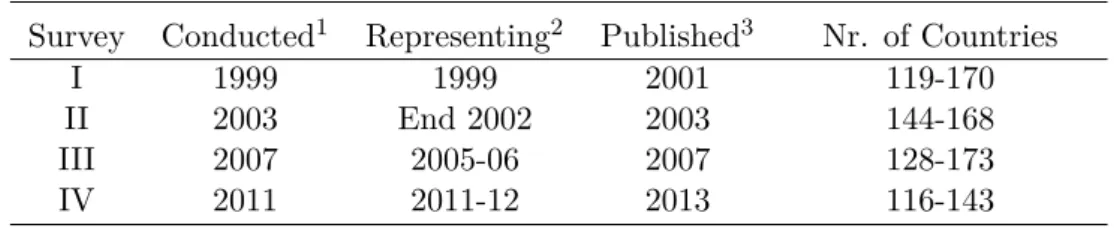
The questionnaire was given to several officials to cross-check the answers and gaps were filled when information could be attained from other official sources.¹¹ Due to the lengthy process the surveys do not represent a specific moment, but a time period. Table 1 summarizes meta data on the surveys.

Table 1: Bank Regulation and Supervision survey overview Survey Conducted¹ Representing² Published³ Nr. of Countries

I 1999 1999 2001 119-170

II 2003 End 2002 2003 144-168

III 2007 2005-06 2007 128-173

IV 2011 2011-12 2013 116-143

The number of countries covered is given as complete cases (lower bound) and cases where at least one answer was given (upper bound) based on the “All Average Scaled Index” considering the variables used in Barth et al. (2012).¹Barth et al., 2013b,²Barth et al., 2012, p. 2,³The World Bank, 2013b.

The World Bank posts the raw survey data of which about 60% are binary questions that are to be answered by “Yes” or “No”, about 35% ask for numeri- cal indicators like the share of government-owned banks, and the rest demands to choose between a set of alternatives.¹² The main survey authors Barth et al. use the survey raw data and improve on each of the four surveys resolving inconsistencies and filling gaps. What is more, they aggregate the data to make it directly usable in research.¹³ The aggregation is important because single binary questions which capture a sub-aspect of e.g. capital regulatory stringency would not be useful as such to explain financial sector differences like bank fragility.¹⁴ Based on their aggregation they conduct own research, e.g. Barth

11Barth, Caprio, & Levine, 2013a, p. 1f

12The World Bank, 2013b

13Barth et al., 2013a, p. 3ff

14To investigate the effect of the three Basel pillars on bank stability one might use many of the binary variables. Following Barth et al. (2013b) this would be 36 variables for the pillars (compare table 2 below). Both the interpretation and the degrees of freedom in the estimation would be a concern.

(7)

2.2 ARE INDICES RELIABLE AND REPRESENT A COMMON FACTOR? 4 et al. (2012) as well as other authors like Boudriga et al. (2009). I attempt to reproduce both papers later on.

2.2 Are indices reliable and represent a common factor?

Investigating the impact of regulation on bank fragility relies on reasonably con- structed indices. Therefore, the index construction should be reviewed. Barth et al. clearly refer to obstacles and limitations in building proper indices, re- ferring to the process as “[t]he Art and Science of Forming Indices”.¹⁵ Even so the authors do not explain and justify their choices. Importantly, the decision which questions enter an index is based solely on theory and the authors’ judg- ment. There is no confirmation based on what the data has to say.¹⁶ Rather, the authors state that the grouping and weighting is not unique and encourage researchers to build their own indices.¹⁷

Methods to build indices At the core of their approach is to take the sum over the questions entering an index. Mostly the questions are asked such that the answer “Yes” stands for more regulatory stringency and is coded with a 1.

One important aspect is how to cope with missing information. Barth et al.

provide two different approaches. There is an “All Index” which gives an index value only when the answers to all underlying questions are provided and an

“All Average Scaled Index” which allows for missing values. The second index is calculated as the mean of the available items¹⁸ where the index value is only given when at least 50% of the underlying questions were answered and more than two questions enter. Based on this methodology and concentrating on the variables used in re-estimating Barth et al. (2012) there are, varying by survey, 119 to 144 complete cases (shown in table 1). For the “All Index” there are only 47 to 87 complete answers. Setting a threshold for the least available item share is reasonable because uncertainty is associated with this procedure. In the extreme, one answer would decide over the index value summarizing many questions. However, the threshold value of 50% might not be optimal and is, again, not discussed by the authors.

Concentration on variables of interest In the rest of the analysis I concentrate on the bank regulatory variables used in the reproduction of Barth et al. (2012) and Boudriga et al. (2009) in section 3 and 4. Table 2 provides the

15Barth et al., 2013a, p. 10

16At least I don’t see a statistical approach mentioned in Barth et al. (2006), Barth et al.

(2013a), or the other publications of these authors mentioned in the references.

17Barth et al., 2006, p. 80f

18The value is then multiplied by the number of questions entering the index such that both indexation methods yield the same measurement scale.

(8)

2.2 ARE INDICES RELIABLE AND REPRESENT A COMMON FACTOR? 5 index definitions and paraphrases the questions the indices consist of. The first three indices represent the Basel pillars capital regulation, official supervision and market discipline. These general aspects of a jurisdiction are represented by ten or more questions. The Capital Regulatory Index tries to capture how limited banks are in using sources as regulatory capital. The first question for this index is in all surveys whether theBasel I capital adequacy regime is used and the answer “Yes” is considered as adding to stringency.¹⁹ For 1999 – where Basel I still had to be refered to as “Basle guidelines”²⁰ – this assignment appears fair. However, in 2011 Basel I was rather out-dated than strict. This exemplifies the difficulty to balance between continuity over time to increase comparability and adequacy of the questions.

Unidimensionality and reliability The indices presented give a single value summarizing the underlying questions. In the special case of a one-variable index no information is removed (lower part of table 2). When different questions are represented by one value the statistic is misleading except for the case where the questions stand for the same underlying concept. We thus require a common factor behind the questions, or unidimensionality.

Imagine a country’s overall stringency in permitted bank activities is to be as- sessed. Therefore restrictions in bank insurance and real estate activities are measured. If high restrictions in one activity are associated with high restrictions in the other we do not reject unidimensionality. If, however, either bank insurance activities or real estate activities are allowed the index is not unidimensional. Then the index value as a summary statistic is not informative about the underlying diverging patterns which might influence bank fragility differently. Statistically, a necessary condition for unidimensionality is a positive correlation of the items entering an index. Table 3 gives for all indices used the number of items which exhibit a negative correlation. Notably, there is not a single index which is free of negative correlation between the items.

Rather, in many cases a considerable share of items shows a negative associa- tion from which I conclude that the indices – or “scales” – offered by Barth et al. are of questionable validity. Using them for analysis introduces a considerable momentum of uncertainty about measuring what we expect to measure.

The main hope is that the overall index value is based on a good theory-driven item selection under which the indices are still informative. E.g. when bank insurance activity restrictions are high while real estate restrictions are not we

19Barth et al., 2013b, Sheet “Index Overview”, No. IV.I

20Barth et al., 2013b, Sheet “Index Overview”, question 3.1.1

(9)

2.2 ARE INDICES RELIABLE AND REPRESENT A COMMON FACTOR? 6

Table 2: Bank Regulation and Supervision survey variable definitions

Index (range) Definition Questions Capital Reg-

ulatory Index (0-10)

Whether capital requirements reflect risk, market value losses reduce capital adequacy and to which scope sources are accepted to initially capitalize a bank.

Is Basel I used? What fraction of revaluation gains is allowed as part of capital? Are unreal- ized losses in fair valued exposures deducted from regulatory capital? Are sources of funds verified by authorities? Can the initial disbursement or subsequent injections of capital be done with assets other than cash or government securities (Yes

= 0)?

Private Mon- itoring Index (0-12)

Measures the incentives and the ability for the private monitoring of firms.

Do banks disclose off-balance sheet items to the public? Are bank regulators/supervisors required to make public formal enforcement actions, which include cease and desist orders and written agreements between a bank regulatory/supervisory body and a banking organiza- tion? To what extent counts subordinated debt as part of Tier 1/Tier 2 capital?

Official Su- pervisory Power (0-14)

Whether the supervisory authorities have the authority to take specific actions to prevent and correct problems.

Do banks disclose off-balance sheet items to supervisors? Can the supervisory agency force banks (a) “to constitute provisions to cover ac- tual or potential losses”? (b) “to reduce or suspend dividends to shareholders”? (c) “to reduce or suspend bonuses and other remuneration to bank directors and managers”? Can the supervisory agency force banks to change its internal organizational structure?

Entry into Banking Re- quirements (0-8)

Whether various types of legal submissions are required to obtain a banking license.

What is legally required before a banking license can be obtained? Draft bylaws, market/business strategy, financial projections, experience of fu- ture Board directors, source of funds to be used as capital.

Overall Re- strictions on Banking Activities (3-12)

The extent to which banks may engage in securities, insurance and real estate activities.

For the three activity categories a ranking de- manded: Can banks directly and fully engage in activities (stringency = 1) up to activities are not allowed in either banks or subsidiaries (stringency

= 4).

Variable range Definition

Government- Owned Banks

0%-100% Percentage of banking system’s assets in banks that are 50% or more government owned.

Foreign- Owned Banks

0%-100% The extent to which the banking system’s assets are foreign owned.

Bank Con- centration (Assets)

0%-100% The degree of concentration of assets in the 5 largest banks.

Bank Regulation and Supervision Survey indices used in Barth et al. (2012) and Boudriga et al. (2009) are shown. Higher values stand for higher stringency. The indices are grouped into those consisting of multiple questions (upper part) and those out of one variable (lower part). The questions are paraphrased based on surveys I-IV and not exhaustive. Range, definitions, and questions are taken from Barth et al. (2013b) and Barth et al. (2013a, Table 5).

(10)

2.2 ARE INDICES RELIABLE AND REPRESENT A COMMON FACTOR? 7 have to assume that in a country with the opposite pattern yielding the same index value the effect on bank fragility is the same to a large extent.

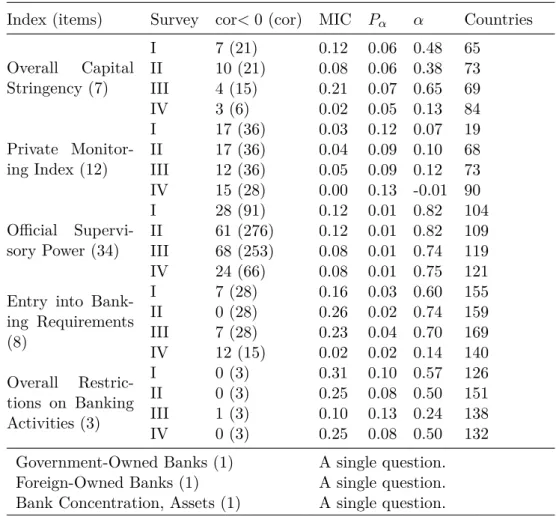
Table 3: Unidimensionality and reliability of the indices

Index (items) Survey cor<0 (cor) MIC P_α α Countries Overall Capital

Stringency (7)

I 7 (21) 0.12 0.06 0.48 65

II 10 (21) 0.08 0.06 0.38 73

III 4 (15) 0.21 0.07 0.65 69

IV 3 (6) 0.02 0.05 0.13 84

Private Monitor- ing Index (12)

I 17 (36) 0.03 0.12 0.07 19

II 17 (36) 0.04 0.09 0.10 68

III 12 (36) 0.05 0.09 0.12 73

IV 15 (28) 0.00 0.13 -0.01 90

Official Supervi- sory Power (34)

I 28 (91) 0.12 0.01 0.82 104

II 61 (276) 0.12 0.01 0.82 109 III 68 (253) 0.08 0.01 0.74 119

IV 24 (66) 0.08 0.01 0.75 121

Entry into Bank- ing Requirements (8)

I 7 (28) 0.16 0.03 0.60 155

II 0 (28) 0.26 0.02 0.74 159

III 7 (28) 0.23 0.04 0.70 169

IV 12 (15) 0.02 0.02 0.14 140

Overall Restric- tions on Banking Activities (3)

I 0 (3) 0.31 0.10 0.57 126

II 0 (3) 0.25 0.08 0.50 151

III 1 (3) 0.10 0.13 0.24 138

IV 0 (3) 0.25 0.08 0.50 132

Government-Owned Banks (1) A single question.

Foreign-Owned Banks (1) A single question.

Bank Concentration, Assets (1) A single question.

Measures of internal consistency and unidimensionality per index and survey. All available items are used to calculate the statistics.

cor<0 (cor) – number of negative item-correlations and in brackets the number of item- correlations in a triangle of the correlation matrix, MIC – mean interitem correlation, Pα – precision of alpha,α – Cronbach’sα, Countries – Number of countries for which all index items were answered in that survey. For the remaining variation in number of correlations compare the note concerning incalculable correlations on page 9.

In the rest of this subsection I exploit finer statistical tools for index appropriateness accompanied by the warning that their validity decreases with a higher share of negatively correlated items. The mean interitem correlation (MIC) tries to capture the extent to which items measure the same.²¹ To get the MIC one can calculate the mean of all entries in the lower triangle of a correlation

21Bühner, 2004, p. 123

(11)

2.2 ARE INDICES RELIABLE AND REPRESENT A COMMON FACTOR? 8 matrix for the variables entering an index.²² I expect the indices to represent a metric latent variable behind the underlying questions. Thus, I use the Bravais-Pearson correlation to calculate the MIC.²³A correlation of.5 might be interpreted as no clear relation. Therefore a MIC of .5 might serve as a crude tool to assess unidimensionality.

The dispersion of correlations is valuable information not considered in the MIC. A small dispersion of the correlations supports the conclusion of a unidimensional index. The precision ofα,

Pα= σM IC

p(1/2∗N ∗(N −1))−1

is a measure for this, whereN is the number of items which enter an index and σ_{M IC} is the standard deviation of the item intercorrelations.²⁴ P_α increases with intercorrelation dispersion and might thus be called “imprecision of α”.

As a rule of thumb, Bühner (2004, p. 123) proposes a threshold of Pα <0.01 as supportive for unidimensionality. Table 3 gives both statistics for the used indices.²⁵ The MIC are all below.5 andP_α is often above 0.01 which indicates a severe problem with multidimensionality in all five indices in the upper part of table 3.

Cronbach’sα is often used in the context of evaluating indices. Related to the MIC it can be written as (Carmines & Zeller, 1979, p. 44)

α= N∗M IC

1 + (N−1)∗M IC.

Essentially the MIC is corrected by the number of itemsN. It can be interpreted as an upper bound for the unidimensionality of the data.²⁶ However, it is unclear how far off the true value the measure is.²⁷ I present Cronbach’s α in table 3. When following Cortina (1993, p. 102) a value of 0.75 should be exceeded to be “acceptable” regardless ofN. Overall, a low value is a sign that there is a problem – and most of the values are below 0.75. A high value, on

22Carmines & Zeller, 1979, p. 44f

23Calculating the MIC based on Spearman’s rank correlation coefficient does not significantly change the picture. One reason for this is that for 0/1-coded variables the Pearson and Spearman correlation are identical.

24Cortina, 1993, p. 100

25The values are calculated based on all available information. The reliability can increase when the share of non-available items in an index is limited. I discuss below that the allowed NA share has a negligible influence on Cronbach’sα.

26Cronbach, 1951, p. 320f

27Cortina (1993, p. 101) alludes to the assumption of “tau-equivalence” of Cronbach’sαwhich can be problematic, Bühner (2004, p. 122f) describes how the measure can be biased from adding items which are not useful and that Cronbach’sαcan be outside the range 0 to 1.

(12)

2.2 ARE INDICES RELIABLE AND REPRESENT A COMMON FACTOR? 9 the other hand, does not show the absence of a problem and thus Cronbach’s α is to be used with caution.²⁸

A necessary condition for an index to be useful is its reliability. According to Bühner (2004, p. 121f) Cronbach’s α gives a lower bound for an index’ reliability. Thus, a highα gives unambigous information about high reliability but an unclear statement about unidimensionality. When the index items are split in halves, more correlation between the parts is a sign for higher reliability.

Cronbach’sα is numerically identical to the mean of all possible split-half correlations.^29,30 Based onα, the official supervisory power index has the highest reliability which is rather stable over the surveys. For some indices reliability appears clearly nonsatisfying. Even under the assumption that the indices are useful without being unidimensional low reliability is an important concern about the presented analysis based on Barth et al. (2013b).

Some of the correlations for table 3 were incalculable. E.g. for overall capital stringency and survey III the question “Is the minimum capital-asset ratio re- quirement risk weighted in line with the 1988 Basle guidelines?”³¹ is answered with “No” only by Nigeria and Venezuela. However, both countries gave no answer in a second question for the index. Computing the correlation for this pair is not possible because the standard deviation in the first question is zero.

In such cases I dropped the variables lacking relevant variation to calculate the measures in table 3.

Varying the share of NA items I noted above that Barth et al. (2013b) use a threshold of 50% as the smallest share of available items allowed when constructing their “All Average Scaled Index”. The threshold is not discussed by the authors. I vary this threshold by 10% steps and control for the change in Cronbach’s α. For official supervisory power the largest difference is obtained for survey IV. Allowing a share of non-available (NA) items of at most 0% (“All Index”), 10%, and 20% yields a Cronbach’sαof 0.71, 0.73, and .75, respectively.

28Another approach to test unidimensionality is factor analysis. Conducting an exploratory factor analysis using principal components based on correlations, the Kaiser criterion proposes for official supervisory power in all surveys at least 5 factors. This is evidence against the appropriateness of assuming one underlying latent variable (a factor). Following the ob- jection that the Kaiser criterion might find too many relevant factors I use Horn’s parallel analysis in which still at least 3 factors are proposed (Bortz & Schuster, 2010, p. 415f).

29Cronbach, 1951, p. 302ff

30Our measures are collected at one point in time and jugded once. When e.g. repeated measurements are available one might measure test-retest reliability. Here we are limited in our choice and test reliability as internal consistency (Cohen, Cohen, West, & Aiken, 2003, p. 129f).

31“(...) with the 1988 Basle guidelines?” is taken from Barth et al. (2013b, Index Overview, question 3.1.1). However, in the Excel file it remains unclear which risk ratio is related to.

This information is taken from the list of guide question in Barth et al. (2006, p. 337).

(13)

2.3 DESCRIPTIVE STATISTICS 10 Increasing the allowed NA share further leaves theαunchanged. Notably, there is no clear pattern over the different indices and surveys that a higher or lower NA share allowed is associated with a higherα. Additionally, the variation inα appears negligible. In conclusion, a threshold of at last 50% NA items appears to be a reasonable compromise between using the collected information and treating a small amount of answers as representative for a hole index. In this regard my statistical analysis supports the indexation by Barth et al. (2013b).

2.3 Descriptive statistics

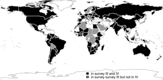
Figure 1 gives an impression of the Barth et al. (2013b) dataset coverage. Coun- tries marked in black are contained in the most recent surveys III and IV while those in grey are only contained in survey III.³² The impression is gained that many African countries left the survey. Though, recognizing that the grey coloured block of central African countries is identical to the members of a financial union³³it appears likely that the block left due to a common decision. I conclude that there is no particular geographical concentration of the countries leaving the survey. Thus there is some evidence to assume random missingness in the sampled countries which is important for the statistical analysis.

in survey III and IV

in survey survey III but not in IV

Figure 1: Coverage of survey III and IV on a world map

Comprehensive coverage of survey III, some fewer countries in survey IV.

32Coverage is measured based on countries giving at least one answer in the “All Average Scaled Index”. Survey III contains the highest number of countries. From survey III to survey IV Ecuador, Gambia, Iraq, Turkey, and Yemen were added.

33The grey block represents the Central African Economic and Monetary Community (CAEMC) consisting of Cameroon, Central African Republic, Chad, Congo, Equatorial Guinea, and Gabon (Barth et al., 2013b, “Groups with uniform bank regulations and supervisory practices”).

(14)

2.3 DESCRIPTIVE STATISTICS 11 Accepting a random country coverage, I am interested in the answer pattern of the sampled countries. One dimension is whether the missingness by question appears to be random; the share of countries for which the indices are available ranges between 66-91% with a standard deviation of about about 10%. I consider the dispersion as not too large. To obtain these values I look at all four surveys, use the “All Average Scaled Index” version, and restrict on the indices used to reproduce Barth et al. (2012) and Boudriga et al. (2009). For the “All Index” – where a missing value in a items leads to a NA for the index – only 47-87% are available with a slightly greater dispersion. Based on these numbers and the findings varying the allowed NA share I use the “All Average Scaled Index” throughout the subsequent analysis.

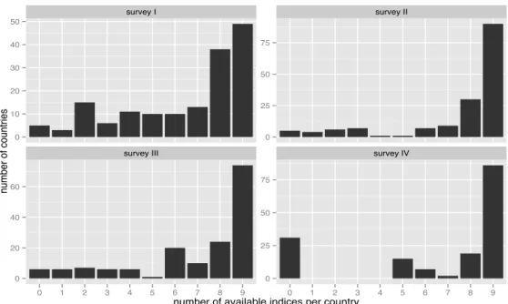
Another dimension is whether the missingness related to answers per country appears to be random. Figure 2 shows that 35 countries gave answers such that 1-4 index values can be calculated in 1999 (survey I). However, zero countries answered in such a way in 2011 (survey IV). Questions added to survey IV due to the financial crisis might have triggered either survey fatigue or the motivation to answer many questions. In this indirect way the change in other survey questions might affect the indices used in the analysis which are build on as tantamount questions as possible to allow comparability over the horizon of over 10 years. Survey IV stands out again as the study answered by the least countries. These issues might flaw the identification of patterns; I assume that this is not the case.

The standard deviations of the three indices representing the Basel pillars are nearly unchanged comparing 1999 and 2011. The mean stringency of capital regulation clearly and of private monitoring marginally increased while mean supervisory power marginally decreased. Underlying the values is a considerable dispersion. Capital stringency (index range is 0-10) was decreased over the 12 years by United Kingdom, Austria, and Mexico by 5 while Venezuela, Turkey, and Bangladesh increased it by 6. In Kazakhstan official supervisory power (index range is 0-14) was decreased by about 8 while Italy increased it by 7.

Private monitoring (index range is 0-12) was decreased by 2 in Portugal but increased by 4 in India and France.³⁴

34The information is obtained from Barth et al., 2013a, figures 9-11. In the paper much more descriptive statistics about the studies are available. Germany increased capital regulations by 2, both official supervisory power and private monitoring by 1, and entry into banking requirements by 4 (only Chile and Finland increased the stringency more).

(15)

3 EXPLAINING NONPERFORMING LOANS (NPL) 12

survey I survey II

survey III survey IV

0 10 20 30 40 50

0 25 50 75

0 20 40 60

0 25 50 75

0 1 2 3 4 5 6 7 8 9 0 1 2 3 4 5 6 7 8 9

number of available indices per country

number of countries

Figure 2: Number of answers in Bank Regulation and Supervision Survey I-IV

Nine of the indices provided by Barth et al. (2013b) are used in the analysis of bank fragility.

The distribution of available indices by survey is shown.

3 Explaining nonperforming loans (NPL)

This section provides a cross-section analysis of the Basel pillars’ impact on nonperforming loans (NPL). The Bank Regulation and Supervision surveys approximately represent certain years and therefore this approach is natural.

First, I attempt to reproduce the results of Barth et al. (2012); this is shown not to be possible due to data issues. The analysis in subsection 3.1 can be seen as a robustness check; while significance differs somewhat the results are in no case contradictory. Subsection 3.2 shows that the dependent should be modeled in logs. Doing so casts doubt on the Barth et al. (2006) finding of a distinctly positive effect of the third Basel pillar, private monitoring. Subsection 3.3 shows that the results are robust to removing outliers while 3.4 introduces an approach to reduce endogeneity in the cross-section setting. Subsection 3.5 investigates differences along income and corruption.

3.1 Reproduction of Barth, Caprio, and Levine (2012)

Barth et al. (2012) investigate the determinants of NPL as a proxy for bank fragility. Their cross-section approach for 1999 and 2011 suffers from a small amount of observations which reduces the chance to obtain significant results.

The upside of this approach is that problems due to incorporating the time

(16)

3.1 REPRODUCTION OF BARTH, CAPRIO, AND LEVINE (2012) 13 dimension are prevented. In their regressions Barth et al. assume that the impact of regulation is the same in all countries,

NPL_i =α+ regulation⁰_iβ+ control⁰_iγ+ui (1) i= 1, . . . , N, for 1999,2011, u_i∼N(0, σ²_i)

whereβ is a vector of dimensionn1×1 andγ of n2×1 wheren1 and n2 stand for the number of regulatory variables and control variables, respectively. The vectors regulation⁰_i and control_i⁰ are correspondingly of dimension 1×n₁ and 1×n2. The error is assumed to be normally distributed with a mean of zero and different variances, i.e. heteroscedasticity.

Definitions and sources of the variables used are shown in table 4. As regulatory and supervisory variables the authors include the Basel accord pillars – capital regulation, official supervision, and market discipline, the last one also called private monitoring – as well as entry requirements and activity restrictions.

Barth et al. skip all non-complete cases: “(...) for countries with missing values, [we] had to drop that observation (...)”.³⁵ The regression output in Barth et al. (2012, p. 17) shows 68 observations entering the ordinary least squares estimation for 1999. Accordingly, at least 68 observations of the regulatory variables without any missing values have to be available.

However, the dataset Barth et al. (2013b) contains only 44 complete cases for the 1999 regulatory variables entering regression 1. I cannot explain this difference; however, I observe that 109 complete cases are available for the “All Average Scaled Index” and I assume that the authors mistook “unscaled” and

“scaled” in their description. I decide to use the richer version of the data which gives index values even when some items are missing.³⁶

The amount and scope of control variables in regression 1 is moderate. Barth et al. use only the countries legal origin.³⁷ NPL are clearly influenced by the economic situation and therefore a time-invariant control variable like legal

35Barth et al., 2012, p. 15

36The working paper was published in December 2012. I received the 2013 dataset from the homepage of one of the authors (Barth et al., 2013b). Data updates in the 2013 version of the data, e.g. due to going back to the authorities and correcting entries, would have increased the complete cases. I assume that the large discrepancies cannot be explained by information that had to be dropped for some reason. The legal origin variables introduced next are available for all countries of survey I and IV and cannot be the reason for the difference.

37The source for the legal origin dummies is not stated in the working paper Barth et al.

(2012). Due to the similar approach I assume that the same source as in their earlier work Barth et al. (2006, p. 191f) is used, namely data from La Porta et al. The co-author Shleifer provides the data on his website (La Porta et al., 2008).

(17)

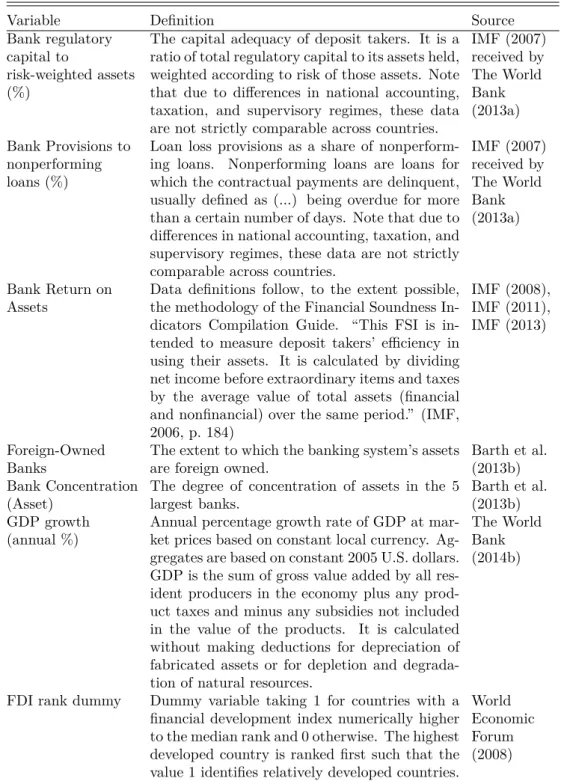
3.1 REPRODUCTION OF BARTH, CAPRIO, AND LEVINE (2012) 14 Table 4: Variable definitions and data sources for Barth et al. (2012)

Variable Definition Original

source Bank

nonperforming loans to gross loans (%), abbreviated:

NPL

Ratio of defaulting loans (payments of interest and principal past due by 90 days or more) to total gross loans (total value of loan port- folio). The loan amount recorded as nonperforming includes the gross value of the loan as recorded on the balance sheet, not just the amount that is overdue. Note that due to differences in national accounting, taxation, and supervisory regimes, these data are not strictly comparable across countries.

IMF (2008) for 2002-04, IMF (2011) for 2005-07, IMF (2013) for 2008-13

Capital Regulatory Index

Whether capital requirements reflect risk, market value losses reduce capital adequacy and to which scope sources are accepted to initially capitalize a bank.

Barth et al.

(2013b)

Private Monitoring Index

Measures whether there are incentives/ability for the private monitoring of firms, with higher values indicating more private monitoring.

Barth et al.

(2013b) Official

Supervisory Power

Whether the supervisory authorities have the authority to take specific actions to prevent and correct problems.

Barth et al.

(2013b) Entry into Banking

Requirements

Whether various types of legal submissions are required to obtain a banking license.

Barth et al.

(2013b) Overall

Restrictions on Banking Activities

The extent to which banks may engage in securities, insurance and real estate activities.

Barth et al.

(2013b) Government-

Owned Banks

Percentage of banking system’s assets in banks that are 50% or more government owned.

Barth et al.

(2013b) Legal origin Dummies for legal origin English, French, Ger-

man, and Scandinavian.

La Porta, Silanes, and Shleifer (2008)

origin appears insufficient. In this section I stick to the authors’ approach while section 4 will use a more comprehensive set of control variables.

Capturing bank fragility with NPL Barth et al. use as dependent variable NPL as a share of total assets. The share increases when NPL increase which puts pressure on the banks’ equity and is thus a good indicator for bank fragility.

Nonetheless, if total assets increase and are used for speculation in less regulated fields, NPL as a share of total assets can go down although risk and bank fragility increase. This calls for a more confined concept. I will use NPL as a share of total loans. Additionally, NPL as a share of total loans is publicly

(18)

3.1 REPRODUCTION OF BARTH, CAPRIO, AND LEVINE (2012) 15 available while the broader concept used by Barth et al. is not.³⁸ NPL as a share of total loans is provided by the International Monetary Fund and is available for 77 and 92 countries in 1999 and 2011, respectively.³⁹ The NPL variable thus provides the least observations in regression 1 and limits the estimation’s scope.

The NPL data comes with a warning: “Due to differences in consolidation methods, national accounting, taxation, and supervisory regimes, data are not strictly comparable across countries.” (IMF, 2013). I translate this additional uncertainty into a need for strong empirical results.

Correlations The common variation of the variables entering regression 1 are shown in table 5. NPL to total loans and the share of government-owned banks represent at least an interval scale of measurement. The indices summing up the individual yes/no-questions are assumed to represent a metric concept. Ac- cordingly, the Bravais-Pearson correlation is used. Spearman’s rank correlation as alternative does, however, not qualitatively change the picture.

Higher values represent higher stringency. In 1999 both capital regulatory stringency and private monitoring are associated with lower bank fragility measured by NPL. In contrast, the second Basel pillar supervisory power is associated with higher bank fragility. In 2011 the common variation between the Basel pillars and NPL is basically lost. Thus, we expect to find a clear impact of the regulation countries adopt and the countries’ NPL level in 1999 while we do not expect a strong impact in 2011. In the aftermath of the financial crisis in 2011 NPL are probably too much affected by contagion, i.e. the financial turmoil which started in the US and spread to other countries regardless of the regulation implemented.

The share of government-owned banks will be added to equation 1 in a second step. In 1999 the correlation of the share of government banks with private monitoring is−.37. This represents that countries with a higher share of government banks – which basically face the same default risk – provide fewer incentives for the market monitoring of risk taking. Because more government banks are (a) associated with more fragility and (b) associated with less private

38NPL as a share of total assets is not available from the World Bank and I was not able to receive it elsewhere in the necessary scope of a variety of the worlds’ countries and the time frame 1999-2011.

39The NPL as a share of total loans for 1999-2011 had to be collected from three sources.

From IMF (2008) to IMF (2011) I noted no differences in overlapping years. However, from IMF (2011) to IMF (2013) some overlapping country series exhibit clearly different numbers. The IMF Data Dissemination and Client Services Team answered to my inquiry that responsibilities changed within the relevant period inducing a change in methodology in April 2011. Whereever data overlaps I use the values from the newest source available.

(19)

3.1 REPRODUCTION OF BARTH, CAPRIO, AND LEVINE (2012) 16 Table 5: Correlations of variables in Barth et al. (2012)

(a) For 1999 / survey I

NPL CapReg PrivMon SupPow Entry ActRes GvtBk

NPL 1

CapReg −0.23 1

PrivMon −0.29 0.13 1

SupPow 0.28 −0.04 0.19 1

Entry 0.12 0.16 −0.11 0.21 1

ActRes 0.38 0.04 −0.09 0.04 0.06 1

GvtBk 0.33 −0.06 −0.37 −0.14 −0.13 0.30 1

(b) For 2011 / survey IV

NPL CapReg PrivMon SupPow Entry ActRes GvtBk

NPL 1

CapReg 0.02 1

PrivMon 0.03 0.15 1

SupPow −0.01 0.11 0.11 1

Entry −0.03 0.07 −0.08 −0.01 1

ActRes −0.17 0.32 0.06 0.19 0.12 1

GvtBk 0.12 0.04 0.01 −0.07 0.02 0.02 1

The common variation of NPL and the three Basel pillars reduced significantly after financial crisis starting in 2007. Higher values of the bank regulatory and supervisory variables stand for more stringent regulation. The “All Average Scaled Index” of Barth et al. (2013b) is used. CapReg is capital regulation, PrivMon is private monitoring, SupPow is supervisory power, Entry are Bank entry requirements, ActRes are overall restrictions on banking activities, GvtBk is the share of government-owned banks.

monitoring linked to more fragility I expect the introduced variable to reduce the significance of private monitoring.

Estimation The most relevant difference compared to Barth et al. (2012) is the dependent NPL to total loans versus their variable NPL to total assets. In this I see the main reason for the different number of observations entering the regressions in table 6. Model 1 uses 62 observations while the original is based on 68.⁴⁰ First, I run the regressions without heteroscedasticity-consistent standard errors and investigate with White’s general test to what extent the variation in the residual variance is a problem. The Null of the test is H₀:σ_i² =σ² for all i, i.e. homoscedasticity. The squared regression residual is explained in a linear regression by the explanatory variables and all of its squares and cross products plus an intercept. The underlying assumption is that the functional terms are

40Adding government banks reduces the observations in the original paper more drastically than in my regressions. As I almost surely have the same information on the share of government banks I think this corresponds to a different country sample selected due to the distinct dependent variable.

(20)

3.1 REPRODUCTION OF BARTH, CAPRIO, AND LEVINE (2012) 17 sufficient to identify any heteroscedasticity. The kind of variation in the errors does not have to be specified.⁴¹ A downside of the test is that the multiplicity of explanatory variables in the auxiliary regression reduces degrees of freedom and can even render the estimation infeasible.

From 62 observations 36 degrees of freedom remain in the case of the first regression in 1999 where I obtain a multiple R² of 41% explaining ˆu²_i. The test statistic isχ²-distributed with nR² ∼ χ²_K(K+1)/2 where K is the number of regressors including the intercept such that n∗R² = 62∗.41 = 25.42 <

χ²_9(9+1)/2 = 51.00 such that the Null of homoscedasticity is not rejected for the baseline regression in 1999.^42,43 Repeating the exercise for 2011, i.e. model 3 in table 6, yields a p-value<0.001 indicating heteroskedasticity in the data.⁴⁴

Table 6: OLS regressions re-estimating Barth et al. (2012)

for 1999 for 2011

(1) (2) (3) (4)

Capital Regulation −0.015^∗∗ −0.014^∗ 0.003 0.003

(0.007) (0.007) (0.004) (0.004)

Private Monitoring −0.021^∗∗ −0.011 0.001 0.002

(0.009) (0.012) (0.005) (0.005) Official Supervisory Power 0.009^∗ 0.007 0.002 0.002

(0.005) (0.006) (0.004) (0.005)

Entry Requirements 0.004 0.007 0.012 0.006

Restrictions on Activities 0.017^∗∗∗ 0.014^∗∗ −0.006^∗ −0.007^∗

Government-Owned Banks 0.001 0.0004

Observations 62 56 76 69

Adjusted R² 0.293 0.264 0.036 0.045

F Statistic 4.166^∗∗∗ 3.191^∗∗∗ 1.348 1.353

∗p<0.1;^∗∗p<0.05;^∗∗∗p<0.01

Dependent variable: nonperforming loans to gross loans. Legal origin variables and the constant are suppressed.

Heteroscedasticity might not be present in all regressions in the reproduction of Barth et al. (2012). Still, the application of heteroscedasticity-consistent standard errors has a minor impact on the inference of a regression without heteroscedasticity. Hence, I follow the original to use a heteroscedasticity consistent (HC) covariance matrix estimation for all regressions. Barth et al. do

41Greene, 2008, p. 165f

42White, 1980, p. 824f, and Wang, 2014

43The probability for the Null (p-value) is 90.1%.

44The example in Greene (2008, p. 167) indicates that White’s test might be quite conservative.

For 1999 homoscedasticity might not be rejected even so it is present. However, applying the Breusch-Pagan/Godfrey LM test using Koenker’s version not sensitive to violations of normality – as proposed in Greene, 2008, p. 166 – yields the same test decisions for the two equations.

(21)

3.2 CAN WE TRUST THE ESTIMATION RESULTS? 18 not state which of the HC estimators they use. HC3 is a variant which builds on White (1980) and tries to additionally correct for a bias due to small samples.

Following the Monte Carlo simulations in Long and Ervin (2000) indicating HC3 to be the best of the alternatives I use HC3 in the cross-section analysis.

The regressions in table 6 confirm the findings from the correlations and the general pattern fits the Barth et al. (2012) results. In 1999 capital regulatory stringency on average significantly decreases bank fragility. More private monitoring has a similar stabilizing effect but the result is less robust as it is lost when controlling for government banks. Theory tells us that the impact of official supervisory power is moderated by the rule of law and corruption in a country.

The only marginal and not robust effect in 1999 is therefore not surprising.⁴⁵ In 2011 (model 3 and 4) the overall F-test cannot reject H0 :β =γ = 0 (compare equation 1) at a level of uncertainty of 10%. This is evidence that after the financial crisis starting in 2007 bank fragility is driven to a large extent by contagion and less by countries’ regulatory decisions.

Beyond a statistical significance we are interested in the effective size of an effect. Observing in model 1 of table 6 a numerically more extreme value for private monitoring than for capital regulation, in absolute terms, cannot be directly evaluated in terms of effect size. The reason lies in the different measurement scales used, e.g. different ranges for the Basel pillars (compare table 2). Among the Basel pillars I expect capital regulation to have the strongest impact on NPL as its coefficient is higher than those of the other Basel pillars which have about the same range. Using standardized regression coefficients confirms the assessment.⁴⁶

3.2 Can we trust the estimation results?

Multicollinearity is present if one of the explanatory variables can mostly be replaced by information in the other regressors. This can have serious conse-

45The impact of activity restrictions on fragility is not clear in theory (Barth et al., 2006) and here found to be positive while not significant in Barth et al. (2012). I don’t consider this further as the research question is the impact of the Basel pillars.

46Standardized regression coefficients are based on the estimated coefficient and “standardize”

by multiplying withsdi/sdN P L, i.e. the standard deviation of the evaluated variable divided by the standard deviation of the dependent (Bring, 1994, p. 210). Bring, 1994, p. 211 criticizes that using both standard deviations and coefficients is inconsistent as coefficient estimates assume the other regressors are held constant and thus relate to another population than the standard deviations based on the full sample. Bring proposes to use the variance inflation factor (VIF) introduced above and jugde coefficients as less relevant when their VIF is higher, i.e. when similar information is contained in other regressors. The result described is obtained based on either the standard formula ˆβi∗(si/sy) or using Brings’

proposal ˆβi∗(sdi/√

V IFi)∗p

n−1/n−k.

(22)

3.2 CAN WE TRUST THE ESTIMATION RESULTS? 19 quences for estimation, t-tests, and inference. Multicollinearity cannot be suffi- ciently identified based on the correlation matrix which shows only collinearity, i.e. the common movement in two variables. I use the Variance Inflation Factor (VIF) as one possible test for the multicorrelation in the independent variables.

The VIF of an independent variable is calculated as V_i = 1/(1−R_(i)² ) where R²_(i) is obtained as the R² regressing xi on a constant and the remaining regressors.⁴⁷ A highR² in this auxiliary regression indicates common movement with one or more of the variables and leads to a highVi value.

In table 6 the regressions contain a dummy variable for English, French and German legal origin while Scandinavian legal origin is omitted to prevent perfect multicollinearity. For all regulatory variables the VIF is below 1.5; values above 5 or 10 are given as rules of thumb indicating a problem. The legal origin dummies give clearly higher VIF up to about 6. As control variables they are included to lessen the omitted variable bias of the parameters of interest.

Notably, multicollinearity in control variables does not affect the estimation of the Basel pillars’ effect on bank stability.⁴⁸ In sum, I reject multicollinearity to harm the identification.

Non-normality In contrast, non-normality of the errors is found to be a severe flaw in the re-estimated regressions. Figure 3 plots quantiles of the OLS residuals against those of the normal distribution. Figure 3a is based on regressions 1 and 3 in table 6, the baseline regressions for 1999 and 2011. Clear deviations particularly in the central part of the distribution are apparent.

I suspect that the strong positive skewness of NPL is an important driver of the model misspecification.⁴⁹ I use a log transformation of the dependent variable to reduce the skewness. As all NPL values are positive we can do so. The log transformation attempts to linearize the relation between the independent variables and NPL. A power transformation chosen more specific to the data would yield a better fit but would come at the cost that both interpretation becomes harder and predictive power can be harmed due to overfitting. Figure 3b shows the normal probability plot for residuals based on the dependent log(NPL), other things equal. Now for 1999 the residuals fit much better to normality. For 2011 the fit improves as well, but to a smaller extent; still a big part in the middle of the distribution does not fit the normal distribution. The

47Mela & Kopalle, 2002, p. 676f

48Von Auer, 2007, p. 488f

49For the variables entering the regressions in Barth et al. the sample skewness attains values of +1.5 and +2.3 for 1999 and 2011, respectively. The values slightly differ by the method used. I employ √

n−1∗m³/(m²)^3/2 where m^r = Pn

i(xi−¯x)^r stands for the sample moments of orderr(e.g. Greene, 2008, p. 1020f).

(23)

3.2 CAN WE TRUST THE ESTIMATION RESULTS? 20

-20 -10 0 10 20

-2 -1 0 1 2

theoretical

sample

-10 0 10 20

-2 -1 0 1 2

theoretical

sample

(a) Dependent variable is NPL for 1999 and 2011, respectively

-2 -1 0 1

-2 -1 0 1 2

theoretical

sample

-2 -1 0 1 2

theoretical

sample

(b) Dependent variable is thelog of NPL for 1999 and 2011, respectively

Figure 3: Normal probability plots for regressions related to Barth et al. (2012)

Plots are for regression 1 and 3 in table 6 (upper left, upper right) and for regression 1 and 3 in table 7 (lower left, lower right).

improved fit can be shown with a normality test on the regression residuals.

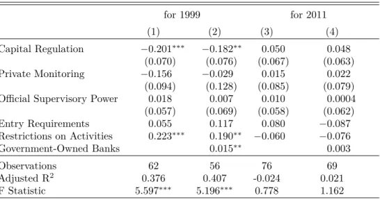
The Shapiro-Wilk tests’ Null hypothesis of normality is rejected for the errors of all models in table 6 (p < .10), i.e. modeling NPL. Yet, modeling log(NPL) yields p-values well above 10% confirming the visual better fit of the errors.⁵⁰ The improved specification modelinglog(N P L) is shown in table 7. The coefficients in 2011 (models 3 and 4) are again not statistically different from zero based on the overall F-test with p =.10 used as threshold. But for 1999 the overall F-test statistic and the adjustedR²increase considerably. Capital regulatory stringency increases bank stability with moderate significance in table 6.

Modelinglog(NPL) capital stringency is identified as a highly significant driver of NPL. Under the inclusion of government banks the result is still significant at

50Shapiro and Wilk (1965, p. 608) find their test to be quite sensitive to deviations, e.g. to asymmetry. The Shapiro-Wilk test has drawbacks for large sample sizes (Shapiro & Wilk, 1965, p. 610) which is no problem here with below 100 observations.