Diagrammatic Monte Carlo for the weak-coupling expansion of non-Abelian lattice field theories: Large-N UðNÞ × UðNÞ principal chiral model
P. V. Buividovich* and A. Davody†
Institute of Theoretical Physics, University of Regensburg, Universitätsstrasse 31, D-93053 Regensburg, Germany
(Received 18 May 2017; revised manuscript received 20 October 2017; published 29 December 2017) We develop numerical tools for diagrammatic Monte Carlo simulations of non-Abelian lattice field theories in the t’Hooft large-Nlimit based on the weak-coupling expansion. First, we note that the path integral measure of such theories contributes a bare mass term in the effective action which is proportional to the bare coupling constant. This mass term renders the perturbative expansion infrared-finite and allows us to study it directly in the large-N and infinite-volume limits using the diagrammatic Monte Carlo approach. On the exactly solvable example of a large-N OðNÞsigma model inD¼2dimensions we show that this infrared-finite weak-coupling expansion contains, in addition to powers of bare coupling, also powers of its logarithm, reminiscent of resummed perturbation theory in thermal field theory and resurgent trans-series without exponential terms. We numerically demonstrate the convergence of these double series to the manifestly nonperturbative dynamical mass gap. We then develop a diagrammatic Monte Carlo algorithm for sampling planar diagrams in the large-N matrix field theory, and apply it to study this infrared-finite weak-coupling expansion for large-N UðNÞ×UðNÞnonlinear sigma model (principal chiral model) inD¼2. We sample up to 12 leading orders of the weak-coupling expansion, which is the practical limit set by the increasingly strong sign problem at high orders. Comparing diagrammatic Monte Carlo with conventional Monte Carlo simulations extrapolated to infinite N, we find a good agreement for the energy density as well as for the critical temperature of the“deconfinement”transition. Finally, we comment on the applicability of our approach to planar QCD at zero and finite density.
DOI:10.1103/PhysRevD.96.114512
I. INTRODUCTION
An infamous fermionic sign problem in Monte Carlo simulations based on sampling field configurations in the path integral is currently one of the main obstacles for systematic first-principle studies of the phase diagram and equation of state of dense strongly interacting matter as described by quantum chromodynamics (QCD). This problem has motivated the search for alternative simulation algorithms for non-Abelian gauge theories, which would hopefully avoid the sign problem or make it milder.
One of the alternative first-principle simulation strategies is the so-called Diagrammatic approach[1], conventionally abbreviated as DiagMC, which stochastically samples the diagrams of the weak- or strong-coupling expansions, rather than field configurations. DiagMC algorithms, com- plemented with the “worm” algorithm techniques [2], turned out to be very helpful for eliminating sign problem in physical models with relatively simple weak- or strong- coupling expansions. The physical models and theories which were successfully studied using DiagMC range from strongly interacting fermionic systems [3–9] relevant in condensed matter physics, via scalar field theories[10–14],
toOðNÞandCPN−1nonlinear sigma models[15–18]and Abelian gauge theories with fermionic and bosonic matter fields [19–21], which are more similar to QCD. This selection of references is by no means exhaustive.
This success has motivated various attempts to apply DiagMC to simulations of non-Abelian lattice gauge theories at finite density [22–28] or the effective models thereof [29–31]. Despite significant progress, these attempts have not so far resulted in a first-principle, systematically improv- able simulation strategy. At the qualitative level, one of the most successful strategies is based on the strong-coupling expansion of lattice QCD, which captures such nonpertur- bative features of QCD as confinement, chiral symmetry breaking and the baryon and meson bound states already at the leading order [32,33]. DiagMC simulations of lattice QCD with staggered fermions at infinitely strong coupling are free of the sign problem in the massless limit, and allow one to reproduce the expected qualitative features of the QCD phase diagram[23,24]. Unfortunately, an extension of this approach to the finite values of gauge coupling meets conceptual difficulties, as the next orders of the strong- coupling expansion coming from the bosonic part of the action should be incorporated in the DiagMC algorithm manually[24], which becomes more and more complicated for higher orders[26]. Ideally, one would also like to sample the strong-coupling expansion in powers of inverse gauge
*Pavel.Buividovich@physik.uni-regensburg.de
†On leave of absence from IPM, Teheran, Iran.
Ali.Davody@physik.uni-regensburg.de
coupling using DiagMC algorithm. Since on finite-volume lattices the strong-coupling expansion is convergent for all values of coupling, simulating sufficiently high orders should allow to access even the weak-coupling scaling region where lattice theory approaches continuum QCD.
Recent attempts to extend the DiagMC simulations to finite gauge coupling using the method of auxiliary Hubbard- Stratonovich variables[25]or the Abelian color cycles[27]
are very promising, but still not quite practical. Development of practical tools for generating high orders of strong- coupling expansion is, thus, currently an important unsolved problem.
However, in the infinite-volume limit strong coupling expansion is known to have only a finite radius of convergence (see, e.g., [34]). One can, thus, expect that as one approaches the weak-coupling regime, the conver- gence of the strong-coupling series will increasingly stronger depend on the lattice size, which might well make the continuum and infinite-volume extrapolation difficult in practice, especially for the infrared-sensitive physical observables such as hadron masses and transport coeffi- cients. Moreover, in the t’Hooft large-N limit one even expects a phase transition separating the strong-coupling and the weak-coupling phases[35–37]even on the finite- volume lattice. These properties of the strong-coupling expansion might significantly limit the ability of DiagMC to work directly in the thermodynamic limit, which is one of the most important advantages of DiagMC over conven- tional Monte Carlo methods [6,7].
These considerations suggest that the extrapolation to the continuum and thermodynamic limit might be easier for DiagMC simulations based on the weak-coupling expansion. However, the weak-coupling expansion for asymptotically free non-Abelian field theories, such as four-dimensional non-Abelian gauge theories and two- dimensional nonlinear sigma models, has two closely related problems, which make a direct application of a DiagMC approach conceptually difficult at first sight. The first problem are infrared divergences due to massless gluon propagators, which cancel only in the final expres- sions for physical observables. The second problem is the non-sign-alternating factorial growth of the weak-coupling expansion coefficients, which is commonly referred to as the infrared renormalon[38]and cannot be dealt with using the Borel resummation techniques. These factorial diver- gences in the perturbative expansions of physical observ- ables originate in the renormalization-group running of the coupling constant, and have nothing to do with the purely combinatorial factorial growth of the number of Feynman diagrams with diagram order.1 In particular, infrared renormalon behavior persists also in the large-N limit
[39–43], in which the number of Feynman diagrams grows only exponentially with order[44]. It is known that if one stops the running of the coupling at some artificially introduced infrared cutoff scale (e.g., by considering the theory in a finite volume), this factorial growth disappears [45,46], thus, in a sense it is a remainder of IR divergences in perturbative expansion.
Recently infrared renormalon divergences have been given a physical interpretation in terms of the action of unstable or complex-valued saddles of the path integral, along with a resummation prescription based on the mathematical notion of resurgent trans-series [47–52].
Trans-series is a generalization of the ordinary power series to a more general form
hOiðλÞ ¼X
i
e−Si=λXmi
l¼0
logðλÞlXþ∞
p¼0
ci;l;pλp; ð1Þ
where hOiðλÞ is the expectation value of some physical observable as a function of the coupling constantλ,ci;l;pare the coefficients of perturbative expansion of path integral around the i-th saddle point of the path integral with the action Si and l labels flat directions of the action in the vicinity of this saddle. It turns out that non-Borel- summable factorial divergences cancel between perturba- tive expansions around different saddle points i in (1).
Unfortunately, currently no method is available to generate the trans-series(1)for strongly coupled field theories in a systematic way. The resurgent analysis of perturbative expansions has been done so far almost exclusively in the regime where gauge theories or sigma models are artificially driven to the weak-coupling limit by a special compactification of space-time to D¼1þ0 dimensions with twisted boundary conditions[47–52].
The aim of this work is to develop DiagMC methods suitable for the bosonic sector of non-Abelian lattice field theories, which is currently a challenge for DiagMC approach. We develop two practically independent tools, which are finally combined together to perform practical simulations.
The first tool is the resummation prescription which renders the bare weak-coupling expansion in non-Abelian field theories infrared-finite and, thus, suitable for DiagMC simulations which sample Feynman diagrams. This pre- scription is introduced in Sec.II and tested in Sec. IIIon some exactly solvable examples. The basic idea is to work with massive bare propagators, where the bare mass term comes from the nontrivial path integral measure for non- Abelian groups and is proportional to the bare coupling.
By analogy with Fujikawa’s approach to axial anomaly [53], this bare mass serves as a seed for dynamical mass generation and conformal anomaly in non-Abelian field theories which are scale invariant at the classical level.
A similar partial resummation of the perturbative series with the help of the bare mass term is also often used in
1The recent work [9] suggests that renormalon divergences might be absent in two-dimensional asymptotically free fer- mionic theories.
finite-temperature quantum field theory[54,55], in particu- lar, in the contexts of hard thermal loop approximation[56]
and screened perturbation theory [57]. Upon this resum- mation, the weak-coupling expansion becomes formally similar to the trans-series(1), but contains only the powers of coupling and of the logs of coupling only, while the exponential factors e−Si=λ seem to be absent. This expan- sion appears to be manifestly infrared-finite and free of factorial divergences at least in the large-N limit. An exactly solvable example of the OðNÞ nonlinear sigma model demonstrates that our expansion reproduces non- perturbative quantities such as the dynamically generated mass gap (see subsectionIII B).
The second tool, described in Sec. IV, is the general method for devising DiagMC algorithms from the full untruncated hierarchy of Schwinger-Dyson equations [58,59], bypassing any explicit construction of a diagram- matic representation. Here the basic idea is to generate a series expansion by stochastic iterations of Schwinger- Dyson equations. We believe the method to be advanta- geous for sampling expansions for which the complicated form of diagrammatic rules makes the straightforward application of e.g., worm algorithm hardly possible, with strong-coupling expansion in non-Abelian gauge theories being one particular example. In this work, we apply the method to sample the (resummed) weak-coupling expan- sion of Sec.II, which for non-Abelian lattice field theories also has complicated form due to the multitude of higher- order interaction vertices.
As a practical application which takes advantage of both tools, in this work we consider the large-N UðNÞ×UðNÞ principal chiral model on the lattice, which is defined by the following partition function:
Z ¼ Z
UðNÞdgxexp
−N λ
X
hx;yi
2ReTrðg†xgyÞ
; ð2Þ
where integration in the path integral is performed over unitaryN×N matricesgx living on the sites of the square two-dimensional lattice,λis the t’Hooft coupling constant which is kept fixed when taking the large-N limit, and P
hx;yi denotes summation over all pairs of neighboring lattice sites x and y. Numerical results for this model obtained by combining the methods of Secs.IIandIVare presented in Sec. V.
While we expect that our approach can be extended to large-N pure gauge theory without conceptual difficulties, in this proof-of-concept study we prefer to work with the principal chiral model (2). The reason is that while this model exhibits nonperturbative features very similar to those of non-Abelian gauge theories, including dynamical mass gap generation, dimensional transmutation and infra- red renormalons [41,42], it has a much simpler structure of the perturbative expansion than non-Abelian gauge theories. Correspondingly, the DiagMC algorithm is also
simpler to implement. We discuss the extension of our approach to large-N gauge theories and illustrate the expected structure of infrared-finite weak-coupling expan- sion for this case in Sec.VI.
II. INFRARED-FINITE WEAK-COUPLING EXPANSION FOR THE UðNÞ×UðNÞ
PRINCIPAL CHIRAL MODEL
The first step in the construction of lattice perturbation theory is to parametrize the small fluctuations of lattice fields around some perturbative vacuum state. For non- Abelian lattice fieldsgx ∈SUðNÞ the most popular para- metrization is the exponential mapping from the space of traceless Hermitian matrices ϕx to SUðNÞ group:
gx¼expðiαϕxÞ, whereαis related to the coupling constant andgx ¼1is the perturbative vacuum. While all the results in this paper could be also obtained for exponential mapping, for our purposes it will be more convenient to use the Cayley map
gx ¼1þiαϕx
1−iαϕx
¼1þ2Xþ∞
k¼1
ðiαÞkϕkx; ð3Þ
whereϕx are again Hermitian matrices and the value of α will be specified later. Since in this work we will be working in the large-Nlimit in which theUðNÞandSUðNÞ groups are indistinguishable, we omit here the zero trace condition for ϕx and work with UðNÞ group. This will significantly simplify the derivation of Schwinger-Dyson equations in terms ofϕx fields; see subsection IVA.
One of the advantages of the Cayley map is the particularly simple form of theUðNÞ Haar measure (see AppendixB 1 for the derivation):
Z
UðNÞdgx¼ Z
dϕxdetð1þα2ϕ2xÞ−N
¼ Z
dϕxexpð−NTr lnð1þα2ϕ2xÞÞ
¼ Z
dϕxexp
−N
α2Trϕ2xþα4
2Trϕ4xþ
; ð4Þ where the integral on the right-hand side is over all Hermitian matricesϕx and…represent the terms of order Oðα6ϕ6xÞor higher. Thus, the Cayley map provides a unique one-to-one mapping between theUðNÞgroup manifold and the space of all Hermitian matrices. Strictly speaking, one should exclude a single pointgx ¼−1from this mapping, which, however, has zero measure in the path integral. In contrast, for exponential mapping the integration overϕx
should be restricted to a certain region within the space of Hermitian matrices in order to avoid multiple covering of UðNÞ group. In addition, for exponential mapping the
exponentiated Jacobian contains double-trace terms [60], which make the planar perturbation theory technically somewhat more complicated (see Appendix B 2). The Cayley map was also used in the context of lattice QCD in the Landau gauge [61–64] and for studying unitary matrix models[65].
The classical action of the principal chiral model(2)can be rewritten in terms of the fields ϕx as
S0¼λ−1X
x;y
ΔxyTrðg†xgyÞ
¼4λ−1Xþ∞
k;l¼1
ð−iαÞkðiαÞlX
x;y
ΔxyTrðϕkxϕlyÞ
¼4λ−1Xþ∞
k;l¼1 kþl¼2n
ð−1Þk−l2αkþlX
x;y
ΔxyTrðϕkxϕlyÞ; ð5Þ
where we have introduced the lattice Laplacian operator in D-dimensional Euclidean space,
Δx;y¼2Dδx;y−XD−1
μ¼0
δx;y−μˆ−XD−1
μ¼0
δx;yþμˆ; ð6Þ
and used the unitarity of gx to add the diagonal terms Trðg†xgxÞ ¼N to the action. Hereμ¼0, 1 labels the two lattice coordinates, andμˆ denotes the unit lattice vector in the direction μ. We see now that in order to get the canonical normalization of the kinetic term in the action S0¼12P
x;yϕxΔx;yϕyþ , where … denotes the terms with more than two fieldsϕ, we have to setα2¼λ8. We also note that the classical action(5)is invariant under the shifts of the field variable ϕx→ϕxþcI, whereI is the N×N identity matrix. This symmetry is a consequence of the scale invariance of the classical action of the principal chiral model.
Rewriting the path integral in the partition function(2)in terms of the new fields ϕx, we also need to include the Jacobian(4). Adding the expansion of the Jacobian(4)in powers ofλandϕto the classical action(5), we obtain the full action for the fieldsϕx:
S½ϕ ¼1 2
X
x;y
Δxyþλ
4δxy
TrðϕxϕyÞ
þXþ∞
k¼2
ð−1Þk−1 λk k8k
X
x
Trϕ2kx
þ Xþ∞
k;l¼1 kþl¼2n;kþl>2
ð−1Þk−l2 4λkþl−22 8kþl2
X
x;y
ΔxyTrðϕkxϕlyÞ; ð7Þ
so that the partition function(2) reads
Z¼ Z
dϕxexpð−NS½ϕÞ: ð8Þ The observation which is central for this work is that the Jacobian(4)contributes a term
λ 8
X
x
ϕ2x ¼m20 2
X
x
ϕ2x ð9Þ
to the quadratic part
SF½ϕ ¼1 2
X
x;y
Δxyþλ
4δxy
TrðϕxϕyÞ
≡1 2
X
x;y
ðΔxyþm20δxyÞTrðϕxϕyÞ
≡1 2
X
x;y
ððG0Þ−1ÞxyTrðϕxϕyÞ ð10Þ
of the action(7), which endows the fieldϕx with the bare massm20¼4λ. Thus, the effect of the Jacobian(4)is to break the shift symmetry ϕx →ϕxþcI of the classical action, serving as a seed for dynamical scale generation and conformal anomaly in the principal chiral model(2).
A conventional approach in lattice perturbation theory, which constructs weak-coupling expansion as formal series in powers of couplingλ, is to treat the quadratic term(9)in the action(7)as a perturbation [66]on top of the kinetic term. Perturbative expansion then involves massless propa- gators ðΔ−1Þxy coming from the scale-invariant classical part of the action, which leads to infrared divergences in the contributions of individual diagrams. These infrared divergences, however, cancel in the final results for physical observables [66]. Furthermore, the resulting power series in the coupling constantλcontain factorially divergent terms, some of which have nonalternating signs and, thus, cannot be removed by Borel resummation techniques. The only recently proposed way to deal with these divergences is to use the mathematical apparatus of resurgent trans-series[47–52].
In this work, we consider a different approach to the weak-coupling expansion based on the action (7), some- what similar in spirit to the screened perturbation theory [54,55,57] and to hard thermal loop perturbation theory [56,67]. Namely, we include the massm20¼λ4coming from (9) into the bare lattice propagators G0xy¼ ðΔþm20Þ−1xy which are used to construct the weights of Feynman diagrams. This corresponds to a trivial resummation of an infinite number of chain-like diagrams with“two-leg” vertices. Since this prescription puts the couplingλboth in the propagators and vertices, we need to define the formal power counting scheme for our expansion. To this end, we group together the terms with the products of ð2vþ2Þ fields, v¼1;2;…þ∞, which correspond to interaction
vertices with ð2vþ2Þ legs, and multiply them with the powersξvof an auxiliary parameterξwhich should be set to ξ¼1to obtain the physical result:
SI½ϕx ¼Xþ∞
v¼1
−λ 8
v
ξvSð2vþ2ÞI ½ϕx; ð11Þ
Sð2vþ2ÞI ½ϕx ¼ m20 2ðvþ1Þ
X
x
Trϕ2vþ2x
þ1 2
X
2vþ1
l¼1
ð−1Þl−1X
x;y
ΔxyTrðϕ2vþ2−lx ϕlyÞ; ð12Þ
where, in the last equation, we have used our definition m20¼4λin order to formally eliminate the couplingλfrom interaction verticesSð2vþ2ÞI ½ϕx. This construction is similar to the“shifted action”of [68].
Perturbative expansion of any physical observable hO½ϕxi is then organized as a formal power series expansion in the auxiliary parameter ξ in(11):
hO½ϕxi ¼lim
ξ→1 lim
M→∞
XM
m¼0
ξm
−λ 8
m
Omðm0Þ; ð13Þ whereMis the maximal order of the expansion. This means that we ignore the relation between the massm20¼λ4and the coupling constantλand treat the termsSð2vþ2ÞI ½ϕxas bare vertices with2vþ2legs, counting only those powersλvof the t’Hooft coupling constant which come from the vertex pre-factors in (11). The bare mass m20 in the expansion coefficients in(13)is substituted withλ=4at the very end of the calculation.
Let us discuss the general structure of an expansion(13) for the free energy of the two-dimensional principal chiral model (2) in the large-N limit, in which only connected planar Feynman diagrams with no external legs contribute.
Consider such a planar diagram with f−1 independent internal loop momenta q1;…; qf−1, and with l bare propagators and vvertices. The kinematic weight of such a diagram can be written as
WK∼ Z
d2q1…d2qf−1 V1…Vv
ðΔðQ1Þ þm20Þ…ðΔðQlÞ þm20Þ; ð14Þ whereQ1…Qlare momenta flowing through each diagram line,
ΔðQÞ ¼XD−1
μ¼0
4sin2 Qμ
2
ð15Þ
is the lattice Laplacian (6) in momentum space which behaves asΔðQÞ∼Q2at small momenta andV1…Vv are
the weights of the vertices which in general depend on q1…qf−1. The momenta Q1…Ql are in general not independent and can be expressed as some linear combi- nations ofq1;…; qf−1. All momenta belong to the Brillouin zoneQμ∈½−π;πof the square lattice. Thus, any possible ultraviolet divergences in the integral(14)are regulated by the lattice ultraviolet cutoffΛUV∼1, and we only have to care about infrared divergences. Each vertex in (14) contributes either a power of m20 or a square of some combination of momentaq1…qf−1, coming from the first or the second terms in (12), respectively. If our planar Feynman diagram is considered as a planar graph drawn on the sphere, the number f is the number of faces of this planar graph. We now take into account the identity f−lþv¼2for the Euler characteristic of a planar graph.
Applying now the standard dimensional analysis, we see that the above relation betweenf,landvimplies thatWK can only contain the terms proportional to Λ2UV, m20, m40=Λ2UV and so on, probably times logarithmic terms
∼logðm20Þ. In subsectionIII B, we will explicitly illustrate the importance of these logarithmic terms. No negative powers ofm0 can ever appear.
Remembering now the relationm20¼λ4, and taking into account the powers of coupling associated with vertices, we immediately conclude that the weights of Feynman diagrams in our perturbation theory with the bare mass m0∼λ are proportional to positive powers of λ, times possible logarithmic terms logðλÞm, logðlogðλÞÞm(m >0) and so on. From(12) we see that the combinatorial pre- factor of vertex with2vþ2legs grows at most linearly with v. Since the number of planar diagrams which contribute to the expansion(13)at ordermgrows at most exponentially withm, and the weight of any diagram is both UV and IR finite, contributions which grow facto- rially withmcannot appear in the expansion(13)inD¼2 dimensions.
The numerical results which we present below suggest that (13) is a convergent weak-coupling expansion. At first sight this contradicts the common lore that pertur- bative expansion cannot capture the nonperturbative physics of the model (2). Let us remember, however, that our expansion is no longer a strict power series inλ, which is known to be factorially divergent. Rather, the mass term m20∼λ in bare propagators allows for loga- rithms of coupling in the series, in close analogy with resummation of infrared divergences in hard thermal loop perturbation theory [67]. It is easy to convince oneself that the formal expansion which contains powers of logs of coupling along with the powers of coupling can incorporate the nonperturbative scaling of the dynamical mass gap
m2∼exp
− 1 β0λ
; ð16Þ
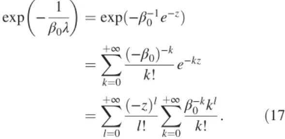
where β0 is the first coefficient in the perturbative β-function. Indeed, we can rewrite the function (16) as a convergent expansion in powers of z¼logðλÞ:
exp
− 1 β0λ
¼expð−β−10 e−zÞ
¼Xþ∞
k¼0
ð−β0Þ−k k! e−kz
¼Xþ∞
l¼0
ð−zÞl l!
Xþ∞
k¼0
β−k0 kl
k! : ð17Þ In what follows, we apply this resummation prescription to construct the infrared-finite weak-coupling expansion for several models: exactly solvable large-N OðNÞsigma model inD¼1, 2, 3 dimensions, exactly solvable large-N principal chiral model on one-dimensional lattices with L0¼2, 3, 4 lattice sites, and, most importantly, the principal chiral model in D¼2 dimensions at zero and finite temperature.
III. EXACTLY SOLVABLE EXAMPLES AND COUNTEREXAMPLES
A. Large-N OðNÞsigma model inD= 1, 2, 3 dimensions
Large-N OðNÞsigma model provides one of the simplest examples of a nonperturbative quantum field theory which can be exactly solved by using saddle point approximation.
InD¼2dimensions, this model has dynamically generated nonperturbative mass gap, similarly to the more complicated principal chiral models and non-Abelian gauge theories.
On the other hand, for this model one can also explicitly construct the formal weak-coupling perturbative expansion, which is dominated by the “cactus”-type diagrams, sche- matically shown in Fig.1. These properties make this model an ideal testing ground for the infrared-finite weak-coupling expansion described in Sec. II.
The partition function of the OðNÞ sigma model is given by the path integral over N-component unit vectors nax,a¼0…N−1attached to the sites ofD-dimensional square lattice, which we label byx:
Z¼ Z
Dnxexp
−N 2λ
X
x;y;a
Δxynaxnay
; ð18Þ
where Δx;y is again the lattice Laplacian (6). The well- known saddle-point solution shows that the two-point correlation function Gxy¼ hnaxnayi is proportional to the propagator of a free massive scalar field, with the mass mbeing the solution of the gap equation:
λI0ðmÞ ¼1; I0ðmÞ≡
Z dDp ð2πÞD
1
ΔðpÞ þm2: ð19Þ InD¼1, 2, 3 dimensions, the functionI0ðmÞ is
I0ðmÞ ¼ 8>
><
>>
:
2m1 ð1þm42Þ−1=2; D¼1;
−4π1logðm322Þð1þOðm2ÞÞ; D¼2;
AþBmþ ; D¼3;
ð20Þ
where in the last lineA¼0.252731andB¼−0.0795775. If the mass gap m is small enough, the corresponding solutions form read
m2ðλÞ ¼ 8>
><
>>
:
ffiffiffiffiffiffiffiffiffiffiffiffiffi λ2þ4
p −2; D¼1;
32expð−4πλÞ; D¼2;
m¼ jB−1jðA−1=λÞ; D¼3.
ð21Þ
The goal of this section is to construct the infrared-finite weak-coupling expansion following the prescription of Sec. II. In order to parametrize the fluctuations of the nax field around the classical vacuum with n0x ¼1, we use the stereographic projection from the unit sphere inN-dimensions toN−1-dimensional real space of fields ϕix,i¼1;…; N−1, which is the analogue of the Cayley map(3):
n0x ¼1−4λϕ2x
1þλ4ϕ2x
; nix¼ ffiffiffiλ p ϕix
1þ4λϕ2x
; ð22Þ
whereϕ2x≡P
iϕixϕix. This is a unique map between the unit sphere embedded in N-dimensional space and the N−1- dimensional real space, in which only a single point with n0x¼−1,nix¼0is excluded. The integration measure on the unit sphere can be written in terms of the stereographic coordinatesϕixas[60](see also AppendixB 3):
Dnx ¼Dϕx
1þλ
4ϕ2x
−N
: ð23Þ
Following the construction of Sec.II, we now include this Jacobian in the action for the fieldsϕix, which reads:
FIG. 1. Feynman diagrams which contribute to the two-point correlator in the large-N limit of the OðNÞsigma model.
S½ϕ ¼1 2
X
x;y
Δxyþλ
2δxy
ðϕx·ϕyÞ
þXþ∞
k;l¼0 kþl≠0
ð−1Þkþlλkþl 2·4kþl
X
x;y
Δxyðϕ2xÞkðϕ2yÞlðϕx·ϕyÞ
þXþ∞
k¼2
ð−1Þk−1λk 4kk
X
x
ðϕ2xÞk; ð24Þ
where ϕx·ϕy≡P
iϕix·ϕiy. We have also taken into account that the terms of the formP
x;yΔxyðϕ2xÞkðϕ2yÞlvanish at largeNdue to factorization propertyhðϕx·ϕyÞðϕz·ϕtÞi ¼ hϕx·ϕyihϕz·ϕtiand translational invariance. In full analogy with the derivation of the action(7)in Sec.II, the Jacobian of the transformation from compact to noncompact field vari- ables results in the bare“mass term”m20¼λ=2.
A convenient way to arrive at the perturbative expansion for the action (24) is to iterate the corresponding Schwinger-Dyson equations
G−1ðpÞ ¼ΔðpÞ þm20−ΔðpÞηð2þηÞ ð1þηÞ2
−λ 2
η 1þη−λ
2 1 ð1þηÞ3
Z dDq
ð2πÞDΔðqÞGðqÞ;
η≡λ
4hϕ2xi ¼λ 4
Z dDp
ð2πÞDGðpÞ; ð25Þ which in the large-N limit involve only the two-point function
hϕx·ϕyi ¼
Z dDp
ð2πÞDeipμðx−yÞμGðpÞ: ð26Þ The form of Eq.(25)suggests that the solution has the form of the free scalar field propagator with the mass m, times some wave function renormalization factor z:
GðpÞ ¼ z
ΔðpÞ þm2: ð27Þ Substituting this ansatz in (25), we obtain the following equations for mand z:
m2¼m20z2−λξ 2 z2þλξ
2 zm2I0ðmÞ;
z¼1þλξ
4 z2I0ðmÞ; ð28Þ where we have again introduced the auxiliary parameterξ, to be set to ξ¼1, in order to define the formal power counting scheme. Substituting ξ¼1 and m20¼λ=2, we immediately arrive at the exact solutions(21)for the mass m. For zthe exact solution is simplyz¼2.
On the other hand, we can use the Eq. (28) for an iterative calculation of the coefficients of the formal weak- coupling expansion
m2¼m20þλξσ1ðm0Þ þλ2ξ2σ2ðm0Þ þ ;
z¼1þλξz1ðm0Þ þλ2ξ2z2ðm0Þ þ ; ð29Þ which is also the formal power series in the auxiliary parameterξin(28). In practice, we continue the iterations up to some finite order M, and calculate m2 and z by summing up all the terms in the series(29)with powers ofξ less than or equal toM. After such a truncation of series, we substituteξ¼1andm0→λ=2.
In D¼1 dimensions, our prescriptions yields the series with summands of the form λkð8þλÞ−M−2 and λkþ1=2ð8þλÞ−M−3=2, k¼1;2;…, times some integer- valued coefficients which depend on M. The expansion, thus, behaves regularly in the limitλ→0, where the mass goes to zero linearly inλ.
In D¼2 dimensions, we get the expansion which involves both powers ofλ and logðλÞ(see also[60]):
m2ðλ; MÞ ¼XM
l¼0
−log λ
64
l Mþminðl;1ÞX
k¼minðlþ2;MÞ
σl;kλk; ð30Þ
and similarly forzðλ; MÞ. As discussed above, the expan- sion involving the logs ofλcan reproduce the nonpertur- bative scaling (21)of the mass gap in D¼2. Finally, in D¼3 dimensions we obtain the expansion in positive powers of ffiffiffi
pλ .
In Fig.2, we compare the convergence of the expansions inD¼1, 2, 3 dimensions, plotting the relative error
ϵðmðλ; MÞÞ ¼mðλ; MÞ−mðλÞ
mðλÞ ð31Þ
of the truncated series(29)with respect to the exact result mðλÞgiven by(21). The values of the couplingλare fixed in such a way that the exact nonperturbative mass gap is equal tom¼0.4for all dimensionsD¼1, 2, 3. The series (29)exhibit the fastest convergence atD¼1. At D¼2, the convergence is not monotonic, and also slower than in D¼1. InD¼3the convergence is slowest, and from the convergence plot in Fig. 2 it is difficult to say whether the series converge or not, even with up to 500 terms in the expansion. These results suggest that for the large-N OðNÞ sigma model D¼2 seems to be the critical dimension separating the convergent and nonconvergent expansions.
B. Nonperturbative mass gap in the two-dimensionalOðNÞ sigma model
We now turn to the physically most interesting example of the two-dimensionalOðNÞsigma model in the large-N
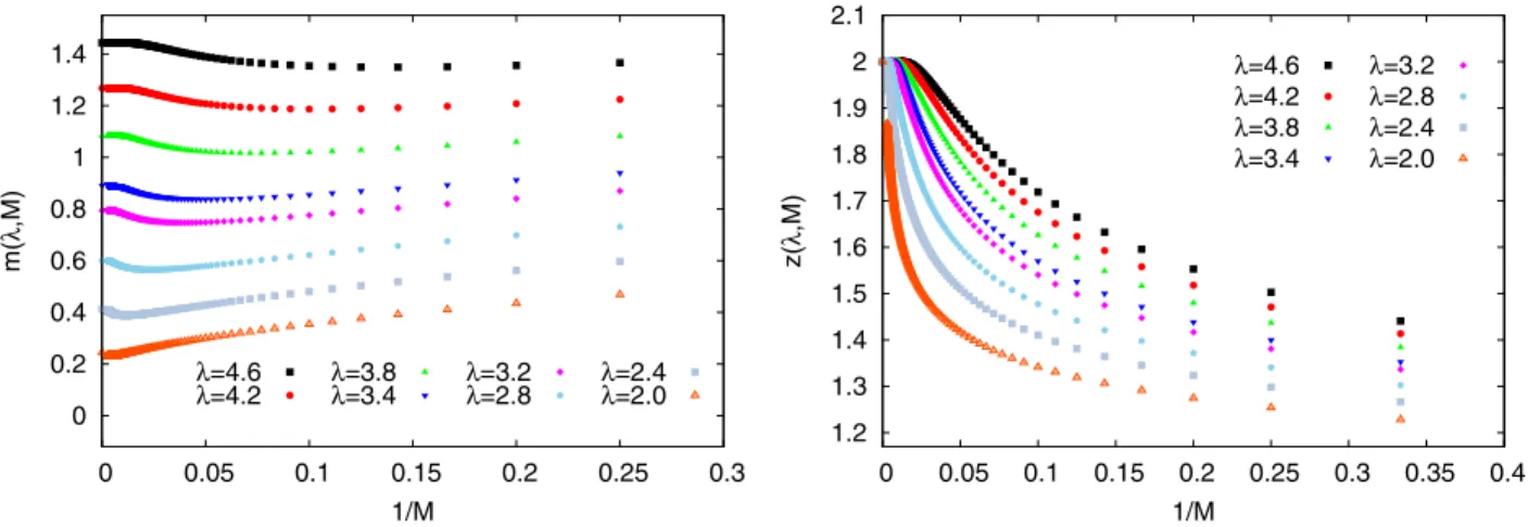
limit, where the mass gap (21) exhibits nonperturbative scaling m2∼expð−β10λÞ similar to the one found also in two-dimensional principal chiral model and in non-Abelian gauge theories. In Fig.3, we illustrate the convergence of the series (30) for the mass m and the renormalization factor z to the exact results (21) and z¼2 for different values of the coupling constantλ. To make the convergence at large truncation ordersMmore obvious, in Fig.4we also show the relative error(31)of the truncated series(30)as a function ofMin logarithmic scale for several values ofλ. While at large values of λ the series converge with the precision of 10−16 at M∼500, the convergence becomes slower at smaller values of λ—and, correspondingly, at smaller values of the mass m.
An interesting feature of the dependence ofmðλ; MÞon M is that it is not monotonous, but rather has several extrema with respect to M. We denote the smallest value of M at which the dependence of mðλ;MÞ on M has a
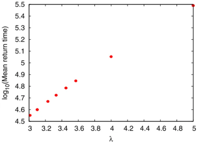
minimum asM⋆1, the position of the next maximum of this dependence—asM⋆2, and so on. These positions depend on λand shift towards largerMat smaller λ. We can think of the extrema positionsM⋆1; M⋆2;…as of some characteristic scales which determine the convergence rate of the trun- cated series. In particular, atM > M⋆1the convergence to the exact value is rather fast. Remarkably, we have found thatM⋆1 as a function ofλwith good precision appears to be proportional to the square of correlation length (in lattice units):
M⋆1∼l2c∼m−2∼exp 4π
λ
: ð32Þ
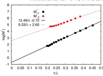
For illustration, in Fig.5we plot logðM⋆1;2ðλÞÞversus1=λ, together with the linear fits of the form logðM⋆ðλÞÞ ¼ const−β=λ. ForM⋆1 the best fit yields the coefficientβ¼ 12.49which is very close to 4π¼12.57. ForM⋆2 we get the best fit value β¼9.33, which is close to 3π¼9.42 and suggests the scaling M⋆2∼l3=2c ∼m−3=2. This might imply that at sufficiently smallλ the two extrema might merge. However, forM⋆2, we have fewer data points, and those exhibit some tendency for faster growth at larger values of1=λ, thus, the scaling exponent forM⋆2might be different at asymptotically smallλ.
The data presented in Figs. 4 and 5 provide a clear numerical evidence that the infrared-finite weak-coupling expansion (30) indeed incorporates the nonperturbative dynamically generated mass gapm2¼32expð−4πλÞ. If we were to sample the series(30) using DiagMC algorithm, the linear scaling ofM⋆1ðλÞwith correlation length would also result in the expectable critical slowing down of simulations near the continuum limit.
The series which we obtain from the field-theoretical weak-coupling expansion(29)based on Schwinger-Dyson equations(28)are in this respect drastically different from
0 0.2 0.4 0.6 0.8 1 1.2 1.4
0 0.05 0.1 0.15 0.2 0.25 0.3
m(λ,M)
1/M λ=4.6
λ=4.2 λ=3.8
λ=3.4 λ=3.2
λ=2.8 λ=2.4 λ=2.0
1.2 1.3 1.4 1.5 1.6 1.7 1.8 1.9 2 2.1
0 0.05 0.1 0.15 0.2 0.25 0.3 0.35 0.4
z(λ,M)
1/M λ=4.6 λ=4.2 λ=3.8 λ=3.4
λ=3.2 λ=2.8 λ=2.4 λ=2.0
FIG. 3. Convergence of the truncated series (29) to the exact values (21) for the effective mass term m (on the left) and the renormalization factorz(on the right), which are plotted as functions of1=M. The data points at1=M¼0correspond to the exact results(21).
-0.1 0 0.1 0.2
0 0.01 0.02 0.03 0.04
ε(m(λ,M))
1/M D=1
D=2 D=3
FIG. 2. Relative error(31)of the mass gap for theOðNÞsigma model from the truncated expansion (29) as a function of truncation order M for D¼1, 2, 3. The coupling is fixed to yield the massmðλÞ ¼0.4in(21)for all D.
the simplest formal expansion(17)of the exact answer(21) in powers of logs. We have explicitly checked that for this case the positions of the extrema ofmwith respect toMare independent ofλ. In this respect, our infrared-finite weak- coupling expansion(29)seems to be closer to the notion of trans-series.
Let us stress, however, that the series(30)are not trans- series yet, despite formal similarity with (1). In a mathematically strict sense, resurgent trans-series (1) should give a “minimal” representation of a function with optimal convergence. For the large-N OðNÞsigma model, this optimal trans-series representation for the dynamically generated mass is given by a single term m2¼32expð−4πλÞ[see the exact solution(21)]. Thus, the true trans-series for this model consist of only one term, which is enough for convergence! The expansion (30) also converges to the exact result (21), but at a non- optimal rate.2
C. Exactly solvable counter-example:
Finite chiral chain models
The UðNÞ×UðNÞ principal chiral model (2) can be solved exactly in D¼1 dimensions for lattice sizes L0¼2, 3, 4 and L0¼ þ∞ [69]. The first and the last cases can be reduced to the Gross-Witten unitary matrix model[35]. For other two cases, solutions can be found in [69]. For all values of L0 the one-dimensional principal chiral model exhibits a third-order Gross-Witten phase transition at some critical coupling λ¼λcðL0Þ, which separates the strong-coupling and the weak-coupling regimes. In particular, for the mean link hN1Trðg†1g0Þi the exact results in the weak-coupling regimeλ<λc are
1
NTrðg†1g0Þ
¼1−λ
8; ðL0¼2;λc ¼4Þ ð33Þ 1
NTrðg†1g0Þ
¼1 λþ1
2−λ 8−1
λ
1−λ 3
3
2; ðL0¼3;λc¼3Þ:
ð34Þ ForL0¼4, the weak-coupling solution is only available in the implicit form:
1
NTrðg†1g0Þ
¼2 λ−λ
8−2 λδ2;
λc ¼8
π
; ð35Þ
where δ is the solution of the equation πλ8ðEð1−δ2Þ−
δ2Fð1−δ2ÞÞ ¼1 and E and F are the complete elliptic integrals of second and first type, respectively.
These analytic expressions offer the possibility to check the convergence of the infrared-finite weak-coupling expansion of Sec. II for small lattice sizes. Of course, for finite lattices the dimensional analysis following Eq. (14) would not work, and loop integrals will only produce some rational functions of λ instead of logs.
Nevertheless it is interesting to check whether these rational functions provide a good approximation to the exact results (33),(35)and(35). To this end, we have performed exact calculations of the coefficients of the weak-coupling expansion (13), generating them recursively up to some maximal order M from the Schwinger-Dyson equa- tions (50), to be presented in subsection IVA. Such an exact calculation is possible forL0¼2up toM¼16and forL0¼4up toM¼8. Explicit expression for the mean linkhN1Trðg†1g0Þiin terms of the correlators ofϕx matrices
-16 -14 -12 -10 -8 -6 -4 -2
150 200 250 300 350 400 450 500 log10(ε(m(λ, M)))
M λ=4.8
λ=4.2 λ=3.4
FIG. 4. Relative error ϵðmðλ; MÞÞ of the effective mass m obtained from the truncated series(29)at large values of M.
-1 0 1 2 3 4 5 6 7 8
0 0.05 0.1 0.15 0.2 0.25 0.3 0.35 0.4 0.45 0.5 log(M* )
1/λ M*1
M*2 12.49/λ -0.72 9.33/λ + 2.60
FIG. 5. The expansion truncation ordersM⋆1;2ðλÞat which the truncated series(30)have local extrema, plotted as functions of the inverse coupling constantλ−1. Solid lines are the fits of the form logðM⋆ðλÞÞ ¼const−β=λ.
2We thank Ovidiu Costin for pointing out these properties of trans-series to us at the“Resurgence 2016”workshop in Lisbon.
and the prescription for truncating the expansion at some finite orderM are given in subsection VA.
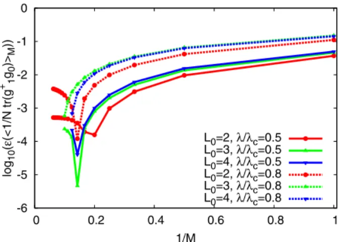
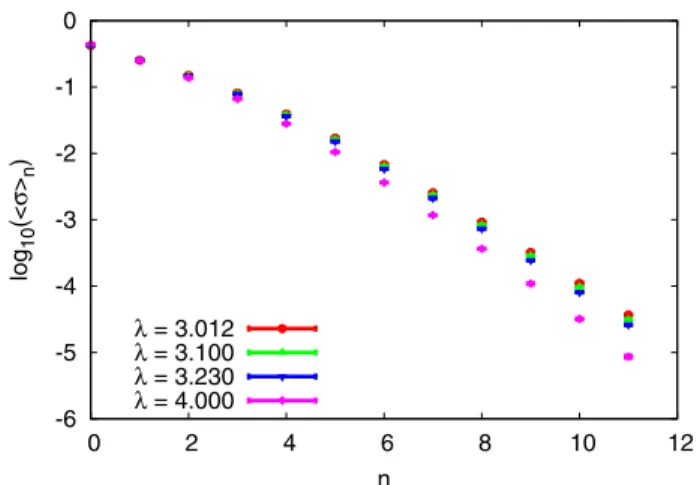
In Fig. 6, we illustrate the relative error of the truncated weak-coupling expansion (13) for the mean link hN1Trðg†1g0ÞiM as a function of inverse truncation order 1=M for L0¼2, 3, 4, fixing λ=λc¼0.5 and λ=λc¼0.8. The relative error is defined in full analogy with (31). At the first sight, the convergence seems to be rather fast; however, a detailed inspection of numerical results reveals a tiny discrepancy of order of 0.1% which cannot be ascribed to numerical round- off errors, and which seems to stabilize at some finite value as M is increased (at least for L0¼2). An analytic calculation of the few first orders revealed that the weak-coupling expansion (13) correctly repro- duces only the three leading coefficients of the standard perturbative expansion in powers of λ, which is con- vergent for finite L0.
It seems, thus, that for finite-size one-dimensional lattices we observe the misleading convergence of the resummed perturbative expansion to some unphysical branch of the solutions of Schwinger-Dyson equations.
This phenomenon might happen even in zero-dimensional models [68] and was first noticed in Bold DiagMC simulations of interacting fermions [70]. Remembering the fact that for the large-N OðNÞ sigma model in the infinite space the expansion (13) converged with much higher precision than the discrepancy which we observe here for finite-size chiral chains (compare Figs.6 and4), we conclude that infinite lattice size and the presence of logðλÞterms seem to be crucial for the convergence to the correct physical result. An important extension of our analysis, which we relegate for future work, would be to extend the sufficient conditions of[68]for the convergence to the physical result to the weak-coupling expansion(13).
IV. SCHWINGER-DYSON EQUATIONS AND DIAGMC ALGORITHM FOR UðNÞ×UðNÞ
PRINCIPAL CHIRAL MODEL
The aim of this section is to construct a DiagMC algorithm for sampling the weak-coupling expansion(13).
While in this work we will only consider the weak-coupling expansion (13) based on the action (7) of the large-N principal chiral model (2), our construction of the DiagMC algorithm is quite general and can be applied to both to the weak and strong-coupling expansions in general large-N matrix field theories. We will briefly outline the extension to non-Abelian gauge theories in Sec.VI.
A. Schwinger-Dyson equations for the large-N UðNÞ×UðNÞ principal chiral model with Cayley
parametrization of UðNÞ group
As in[4,5,8,13,14], the starting point for the construction of our DiagMC algorithm are the Schwinger-Dyson equa- tions, which we derive for the action(7) of the principal chiral model (2). In contrast to the works [13,14]on the bosonic DiagMC, here we consider the full untruncated hierarchy of Schwinger-Dyson equations for multitrace, in general disconnected, correlators of theϕxfields defined in(3):
h½x11;…;x1n1½x21;…;x2n2…½xr1;…;xrnri
≡ 1
NTrðϕx11…ϕx1n1Þ1
NTrðϕx21…ϕx2n2Þ…1
NTrðϕxr1…ϕxrnrÞ
: ð36Þ To derive the Schwinger-Dyson equations for the field correlators (36), let’s consider the full derivative of the form
δikδjl
Nr Z
Dϕ ∂
∂ϕxij
ððϕx12…ϕx1n1Þ
klTrðϕx21…ϕx2n2Þ…
× Trðϕxr1…ϕxrnrÞexpð−SF½ϕ−SI½ϕÞÞ ¼0; ð37Þ where we have explicitly separated the action(7) into the quadratic and interacting parts given by(10)and(11),(12) to simplify the derivation and notation. We now expand the derivative according to the Leibniz product rule, contract matrix indices and finally contract the result with the bare propagatorG0x1
1x¼ ðΔþm20Þ−1xy coming from the quadratic part SF½ϕx of the action (7). This yields the following infinite system of equations for the multitrace observables(36):
h½x1; x2i ¼G0x1x2þX
x
G0x1x ∂SI
∂ϕx
; x2
; ð38Þ
-6 -5 -4 -3 -2 -1 0
0 0.2 0.4 0.6 0.8 1
log10(ε(<1/N tr(g+ 1g0)>M))
1/M
L0=2,λ/λc=0.5 L0=3,λ/λc=0.5 L0=4,λ/λc=0.5 L0=2,λ/λc=0.8 L0=3,λ/λc=0.8 L0=4,λ/λc=0.8
FIG. 6. Relative error of the weak-coupling expansion(13)for the mean linkhN1Trðg†1g0ÞiMof the principal chiral model(2)on the one-dimensional lattices withL0¼2, 3, 4 sites, as a function of truncation orderM for fixedλ=λc¼0.5andλ=λc¼0.8.