How did micro-mobility change in response to COVID-19 pandemic?: A case study based on spatial-temporal-semantic analytics

Research Collection

Working Paper

How did micro-mobility change in response to COVID-19 pandemic?

A case study based on spatial-temporal-semantic analytics

Author(s):

Li, Aoyong; Zhao, Pengxiang; Haitao, He; Mansourian, Ali; Axhausen, Kay W.

Publication Date:

2021-03

Permanent Link:

https://doi.org/10.3929/ethz-b-000473263

Rights / License:

In Copyright - Non-Commercial Use Permitted

This page was generated automatically upon download from the ETH Zurich Research Collection. For more

information please consult the Terms of use.

How did micro-mobility change in response to COVID-19

1

pandemic? A case study based on spatial-temporal-semantic

2

analytics

3

Aoyong Li

, Pengxiang Zhao

, He Haitao

, Ali Mansourian

, Kay W. Axhausen

4

a

Institute for Transport Planning and Systems (IVT), ETH Z¨ urich, Z¨ urich CH-8093, Switzerland

5

b

GIS Center, Department of Physical Geography and Ecosystem Science, Lund University, Lund 22362,

6

Sweden

7

c

School of Architecture, Building and Civil Engineering, Loughborough University, UK

8

d

Center for Middle-Eastern Studies, Lund University, Lund, Sweden

9

Abstract

10

The outbreak of the coronavirus disease 2019 (COVID-19) brought an unprecedented

11

global health crisis. In response to the pandemic of COVID-19, many countries and

12

cities around the world adopted the lockdown policy, which has influenced people’s travel

13

behavior as well as habits and customs. Micro-mobility, as one special type of human

14

mobility, has attracted notable attention in recent studies, while little efforts have been

15

devoted to understanding the changes of micro-mobility in response to COVID-19. In this

16

study, we explore and analyze the changes of micro-mobility behavior before and during

17

the lockdown period by conducting a case study in Zurich, Switzerland. Specifically, the

18

changes of three types of micro-mobility services, namely docked bike, docked e-bike,

19

and dockless e-bike, are considered and compared from the perspective of space, time

20

and semantics. First, the spatial and temporal analysis results uncover that the number

21

of trips decreased remarkably during the Lockdown period, and the striking difference

22

between the Normal and Lockdown period is the decline in the peak hours of workdays.

23

Second, the origin-destination flows of three types of micro-mobility services are used to

24

construct spatially embedded networks. The spatial network analysis results suggest that

25

the movements by micro-mobility services between the PLZs has not been interrupted

26

completely during the Lockdown period, while the numbers of trips between the PLZs

27

are definitely reduced due to COVID-19 pandemic. Finally, the semantic analysis is

28

conducted to uncover the micro-mobility changes in terms of trip purpose. By comparing

29

the proportions of each type of activity during the two periods, it is revealed that the

30

proportions of Home, Park, and Grocery activities increase, while the proportions of

31

Leisure and Shopping activities decrease during the lockdown period. This study can be

32

beneficial for understanding micro-mobility changes in the context of the pandemic, and

33

the implications with respect to urban planning and policy recommendations.

34

Keywords: COVID-19, Micro-mobility, Docked, Dockless, Spatiotemporal analysis,

35

Trip purpose

36

∗

Corresponding Author: Aoyong Li (aoli@ethz.ch)

1. Introduction

37

The pandemic outbreak of novel coronavirus disease 2019 (COVID-19) has caused

38

radical social changes world-wide, and posed a large threat to health, life and livelihood

39

of the populations (Gatto et al., 2020; Kraemer et al., 2020; Oliver et al., 2020). As of

40

October 1, 2020, there had been more than 34,048,240 confirmed cases and 1,015,429

41

deaths around the world. Due to the pandemic, Italy applied a national lockdown in

42

response to the spread of COVID-19 on March 9, 2020 after China, and was also the first

43

European country to implement a lockdown (Bonaccorsi et al., 2020). Following Italy and

44

China, some other countries also conducted national lockdowns successively. For example,

45

Swiss government announced that schools and most shops were closed nationwide from

46

16 March, 2020. During the lockdown period, almost all the public facilities like schools,

47

shops are closed, and all public events are banned. Also, people are requested to work from

48

home and encouraged to stay at home to reduce unnecessary trips (Engle et al., 2020).

49

It is evident that COVID-19 pandemic had a significant impact on human mobility and

50

urban transportation.

51

As low-carbon and micro-mobility transportation modes, bike-sharing services are

52

playing a crucial role in human daily travel, especially in solving first- and last-mile

53

problems. In such a situation, micro-mobility was undoubtedly influenced by the epidemic

54

of COVID-19. On the one hand, to keep social distancing, an increasing number of people

55

chose to stay at home to minimize going out for the dispensable activities during the

56

pandemic period, which implies that the number of trips on micro-mobility would decrease

57

intuitively. On the other hand, people’s intention might have increased to substitute

58

public transportation with micro-mobility transportation modes for the necessary short-

59

or medium-distance trips to reduce the risk of getting infected in public transportation.

60

Therefore, it would be necessary to explore how micro-mobility changes in response to

61

COVID-19 pandemic, which is beneficial for understanding micro-mobility patterns and

62

enhancing the effective scheduling of bikes during pandemic period.

63

In recent years, shared micro-mobility services (e.g., docked and dockless bike-sharing,

64

scooter sharing), as the environmentally friendly travel modes, have attracted consider-

65

able attention in academic and industrial fields, which have proved to be able to facili-

66

tate alleviating traffic congestion and transport-related emissions (Wang and Zhou, 2017;

67

Zhang and Mi, 2018; McKenzie, 2020; Milakis et al., 2020). Especially, with the rapid de-

68

velopment of mobile computing and payment, micro-mobility services have been realized

69

as effective alternatives to short- and medium-distance trips by public and private car

70

transportation. The services allow users to locate and unlock a bike almost everywhere

71

through smartphones and park it after completing the trip. Although micro-mobility

72

services bring convenience for people’s travel, several issues are still facing the city and

73

urban transportation. In particular, considering the various types of micro-mobility ser-

74

vices, including docked and dockless bike, electric bike (e-bike), little is known about

75

the similarity and difference of micro-mobility patterns for different types of services,

76

especially how these micro-mobility patterns change in response to COVID-19 pandemic.

77

The goal of this study is to investigate the variations of micro-mobility before and

78

during the COVID-19 pandemic period by conducting a case study in Zurich, Switzerland.

79

Using a micro-mobility dataset over two months collected by a company in Zurich, we

80

conduct spatial, temporal, and semantic analytics to uncover how micro-mobility changes

81

in response to the COVID-19 pandemic. We divide the dataset into two parts based on the

82

lockdown date, namely the normal (NP) and lockdown (LD) periods. First, the spatial

83

and temporal changes of trips for the three types of micro-mobility services are examined

84

during the two periods. Second, spatial network analysis is conduct to explore the micro-

85

mobility patterns by comparing the three types of services during the two periods from

86

the perspective of human interaction. Third, semantic analytics are implemented to

87

uncover how different types of activities vary before and during the pandemic period for

88

the three types of micro-mobility services. To the best of our knowledge, no previous

89

studies have investigated how micro-mobility use change in response to the COVID-19

90

pandemic, especially in exploring the changes in spatial, temporal, and semantic domains

91

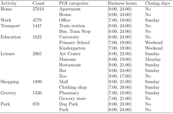
by systematically comparing three types of micro-mobility services.

92

The remainder of this paper is organized as follows. Section 2 reviews human mobility

93

in response to COVID-19, micro-mobility patterns, and trip purposes imputation. Section

94

3 describes the utilized data and short introduction to the data preprocessing. Section 4

95

introduces the methodology of this paper. Section 5 presents the results of micro-mobility

96

changes during Normal and Lockdown period. Finally, we highlight our conclusions and

97

summarize future work in Section 6.

98

2. Literature Review

99

2.1. Human mobility in response to COVID-19

100

Since the outbreak of COVID-19, several studies have been conducted to investigate

101

how human mobility reacts to the epidemic. For instance, Kraemer et al. (2020) examined

102

the effect of human mobility on the COVID-19 epidemic in China using the mobility

103

data from Wuhan and the detailed case data including travel history. The work by

104

Galeazzi et al. (2020) performed a massive data analysis to explore how COVID-19 affects

105

mobility patterns in France, Italy and UK using social media data. It is found that the

106

three countries displayed very different mobility patterns. Beria and Lunkar (2020) used

107

Facebook data to understand the mobility patterns in response to COVID-19 during the

108

lockdown period in Italy. They reported that the share of people movement and the

109

range of movement decreased dramatically. For the sake of estimating how individual

110

mobility is influenced by travel restrictions, Engle et al. (2020) implemented a study

111

by combining GPS location data with COVID-19 case data and population data at the

112

county level. The results indicate that population mobility declined by 7.87% due to

113

the government stay-at-home restriction. The study from Warren and Skillman (2020)

114

utilized the mobility data at the state and county levels in US to detect the mobility

115

changes in response to COVID-19. A large reduction in mobility is identified in the

116

US. Gao et al. (2020) developed an interactive web-based mapping platform to provide

117

information on how mobility pattern changes at the county level in the US in response

118

to COVID-19. Huang et al. (2020) conducted a data-driven analysis to understand the

119

impact of the COVID-19 pandemic on transportation-related behaviors using the massive

120

human mobility data from Baidu Maps. It is found that human mobility patterns changed

121

dramatically during the pandemic period. Molloy et al. (2020) examined the mobility

122

patterns before and after the start of the pandemic in Switzerland using the participants’

123

GPS trajectory data from the MOBIS-COVID-19 tracking study. The drastic reduction

124

in mobility after the implementation of lockdown measures was observed.

125

2.2. Understanding micro-mobility patterns

126

Many studies have explored and analyzed human micro-mobility patterns using GPS-

127

based micro-mobility trajectory data. Most of these studies are concentrated on un-

128

derstanding bike-sharing mobility patterns, which consist of docked and dockless bike-

129

sharing systems. For instance, Wergin and Buehler (2017) examined the travel behaviors

130

of two types of bike-sharing users (i.e., short- and long-term) by analyzing the trips of

131

bikes between docking stations. Xu et al. (2019) uncovered the temporal variations of

132

bicycle usages at various locations in Singapore using an eigendecomposition approach,

133

which indicated different space-time characteristics of cycling activities on weekdays and

134

weekends. Yang et al. (2019) investigated the changes of travel behaviors by analyzing

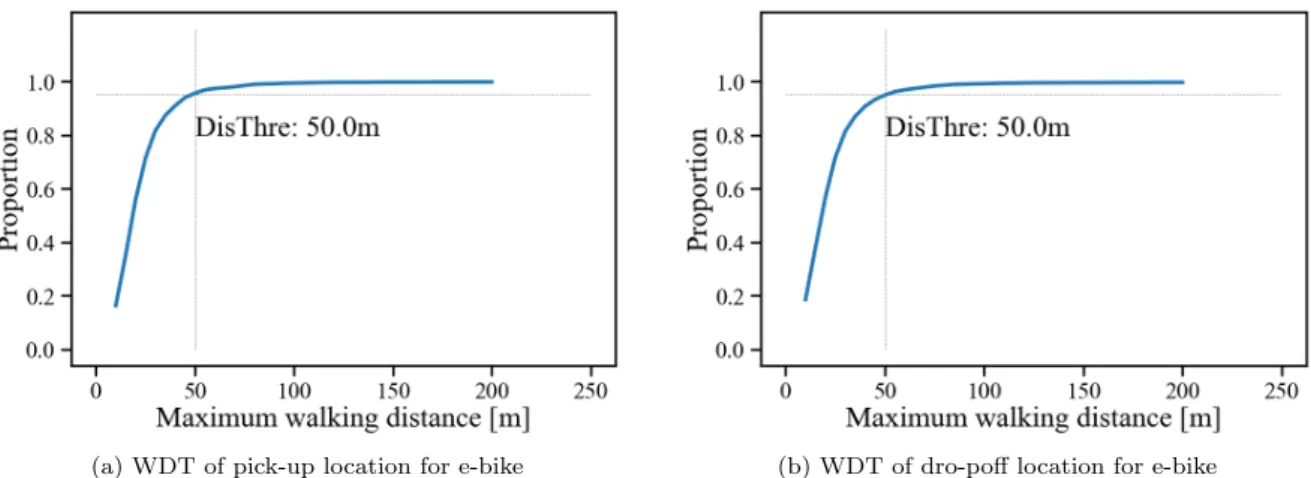
135

bike-sharing during a period when a new metro line came into operation in Nanchang,

136

China. The results showed how the spatiotemporal patterns of bike travel behavior

137

changed over the period. A comparative study was conducted to examine the difference

138

in travel characteristics between docked and dockless bike-sharing systems. It was found

139

that shorter average travel distance and travel time are achieved for dockless bike-sharing

140

systems, while higher use frequency and hourly usage volume are obtained in contrast

141

with docked bike-sharing systems (Ma et al., 2019). Li et al. (2020b) explored dockless

142

bike-sharing utilization pattern and its explanatory factors by implementing an empirical

143

study from the GPS bike origin-destination data in Shanghai.

144

2.3. Predicting trip purpose on micro-mobility

145

As one of the crucial characteristics of human mobility, trip purposes are significant

146

for understanding human travel behavior and estimating travel demands. A large num-

147

ber of studies have been conducted to predict trip purposes using various GPS-based

148

human mobility datasets. For instance, Deng and Ji (2010) presented a machine learning

149

approach to impute trip purposes from GPS track data by combining with other relevant

150

data sources like land use. Lee and Hickman (2014) developed an approach to derive

151

passengers’ trip purposes from the farecard transaction data, which can contribute to the

152

development of heuristic rules for trip purpose inference. The study from Alexander et al.

153

(2015) exploited mobile phone data to infer activity types based on observation frequency,

154

day of week, and time of day, etc. Li and Axhausen (2018) proposed a framework to infer

155

trip purposes from GPS-based taxi trajectory data by considering the location and time

156

of drop-off points as well as the trajectory form. The work by Zhao et al. (2020a) pro-

157

posed a method to identify cabdrivers’ dining activities from GPS taxi trajectory data

158

based on the support vector machine (SVM) algorithm. Overall, rule-based methods and

159

machine learning algorithms are still the mainstream of trip purpose inference.

160

With the booming of bike-sharing systems, several studies were implemented to pre-

161

dict trip purposes from bike-sharing movement data. For instance, Bao et al. (2017)

162

investigated bike-sharing travel patterns and trip purposes by conducting the Latent

163

Dirichlet Allocation (LDA) analysis from bike-sharing smart card data and online point

164

of interests (POIs) data. Li et al. (2020a) applied a Dirichlet multinomial regression

165

topic model (DMR model) to infer trip purposes from bike trajectories by considering

166

arrival time and drop-off location. Xing et al. (2020) investigated the trip purposes of

167

bike-sharing users using the bike-sharing data and online POIs. Specifically, the spatial

168

attractiveness of each POI category within the walkable distance around origin or desti-

169

nation is calculated. Kou et al. (2020) inferred trip purpose by comparing the trip speed

170

to the average speed of all trips in the city, thereby quantifying greenhouse gas emissions

171

reduction from bike share systems. Considering above, little attention has been paid to

172

explore and understand micro-mobility patterns from the perspective of trip purpose,

173

especially during the COVID-19 pandemic.

174

3. Data description and preprocessing

175

3.1. Micro-mobility transaction data

176

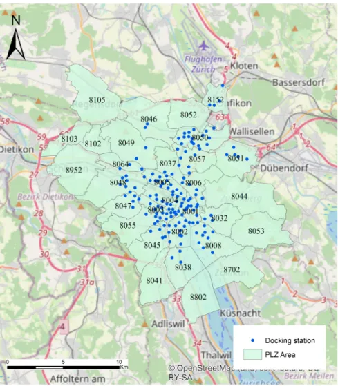
Figure 1 shows our study area, which is divided into 31 sub-regions according to postal

177

codes (PLZ) in Switzerland. The area contains Zurich city (24 PLZs) and surrounding

178

Postal codes zones (7 PLZs). Zurich is one of the big cities and economic centers in

179

Switzerland, with 434k inhabitants.

180

Several micro-mobility services are operating in this area. Here, we use three types

181

of micro-mobility services from two operators. Two of them are docked micro-mobility

182

from Publibike, namely docked bike and docked e-bike. Publibike

is the most established

183

sharing services in Switzerland. The study area contains 153 docking stations (shown in

184

Figure 1). A dockless e-bike service is provided by Bond (formerly Smide

). Compared

185

with publibike e-bikes, Bond e-bikes can travel at a higher speed (up to 45 km/h). This

186

paper aims to explore the change of micro-mobility use before and during the COVID-19

187

pandemic. Considering that most e-scooter services stopped their services after around

188

March 15, 2020 (the date of lockdown), we ignore e-scooter service.

189

Figure 1: Study area

1

https://www.publibike.ch/en/publibike/

2

https://bond.info/en/

The transaction data is collected from micro-mobility companies in Switzerland, which

190

include trips with origins and destinations. Each trip contains ID, start time, start loca-

191

tion, end time, end location, trip duration, and trip distance. Although these transaction

192

data belong to different types of micro-mobility service, the duration of the used trips

193

are between two minutes and one hour. A summary of the data description is listed in

194

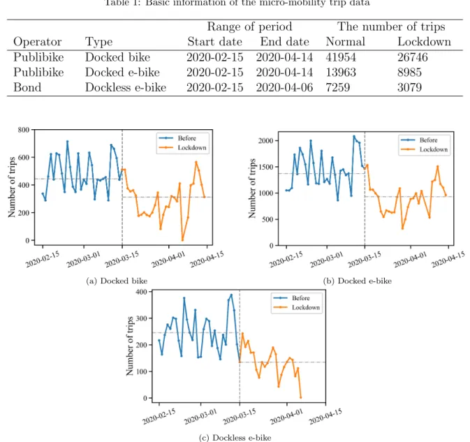
Table 1. The data span from February 15 to April 14, 2020, covering the normal period

195

(February 15 to March 14, 2020) and part of the lockdown period (March 15 to April

196

14, 2020). In this study, the whole period is divided into two parts, denoted as Normal

197

period (NP) and Lockdown period (LD), according to the lockdown date of Switzerland.

198

Figure 2 plots the number of trips for each type of service per day during the two periods.

199

The dashed lines represent the average number of trips during the two periods for each

200

type of micro-mobility service respectively. It can be observed that the average number

201

of trips decreased remarkably during the Lockdown period compared with that of the

202

Normal period, which coincides with the conclusions from previous studies (Molloy et al.,

203

2020).

204

Table 1: Basic information of the micro-mobility trip data

Range of period The number of trips

Operator Type Start date End date Normal Lockdown

Publibike Docked bike 2020-02-15 2020-04-14 41954 26746 Publibike Docked e-bike 2020-02-15 2020-04-14 13963 8985 Bond Dockless e-bike 2020-02-15 2020-04-06 7259 3079

(a) Docked bike (b) Docked e-bike

(c) Dockless e-bike

Figure 2: Number of trips per day for the three types of micro-mobility services during the two periods.

3.2. Point of interest

205

The Point of interest (POI) dataset was extracted from OpenStreetMap

, contain-

206

ing 41322 records. Each POI record has several attributes, including ID, name, type,

207

and location (longitude and latitude). Since business hours are not available in the POI

208

dataset, we assign business hours to each type of POI based on their typical business

209

hours in the study area. In this study, we further divide these POIs into eight com-

210

mon categories, including Home, Work (such as some companies and government offices),

211

Transport (such as tram, bus, and train stations), Education (such as kindergarten, pri-

212

mary school, or university), Leisure (mainly referring to the indoor activities), Shopping

213

(mainly big shops such as malls, clothing shops), Grocery (the shops related to daily life,

214

such as supermarket), Park (mainly refer to facilities providing outdoor activities). Table

215

2 displays the eight POI categories and their assumed business hours.

216

Table 2: POI categories and business hours

Activity Count POI categories Business hours Closing days

Home 27010 Apartment [0:00, 24:00) No

House [0:00, 24:00) No

Work 4779 Office [7:00, 19:00) Sunday

Transport 1447 Train station [0:00, 24:00) No

Bus, Tram Stop [0:00, 24:00) No

Education 1022 University [0:00, 24:00) No

Primary School [7:00, 19:00) Weekend Kindergarten [7:00, 19:00) Weekend

Leisure 2965 Art Center [8:00, 22:00) Sunday

Museum [8:00, 19:00) Monday

Restaurant [9:00, 21:00) Sunday

Bar [0:00, 24:00) Sunday

Zoo [9:00, 17:00) No

Shopping 1899 Mall [9:00, 21:00) Sunday

Clothing shop [7:00, 20:00) Sunday

Grocery 1330 Pharmacy [7:00, 18:00) Sunday

Grocery store [7:00, 21:00) No

Park 870 Dog Park [0:00, 24:00) No

Park [0:00, 24:00) No

3.3. GPS Survey data

217

GPS survey data were collected by the MOBIS study in Switzerland (Molloy et al.,

218

2020). This survey tracked 3700 participants and recorded their trajectories from Septem-

219

ber 2019 to February 2020. In the tracking process, participants were asked to validate

220

their activity information for their stay points. Here, we extract these stay points within

221

the study area, containing 92539 records. Each record has start time, finish time, activity

222

type, and location. These records consist of ten kinds of activities, which are listed in

223

Table 3.

224

3

https://download.geofabrik.de/

Table 3: The activity type in GPS tracking data

Name Count Share (%)

Home 28000 30.26

Work 24737 26.73

Leisure 14135 15.27

Wait 7240 7.82

Shopping 6575 7.11

Errand 5579 6.03

Assistance 3118 3.37

Study 2644 2.86

Home office 271 0.29

Co-working 240 0.26

4. Methodology

225

In this study, we conduct the analytics on how micro-mobility services change from

226

three aspects, including general spatial-temporal analysis, spatial network analysis, and

227

semantic analysis. The spatial and temporal analysis focus on the overall micro-mobility

228

pattern in time and space from a static perspective. The spatial network analysis aims

229

to explore how people move between spatial units from the perspective of interaction.

230

Semantic analysis uncovers micro-mobility patterns by predicting trip purposes and di-

231

viding the trips into different categories based on purpose. Spatial network analysis and

232

semantic analysis based on trip purposes are introduced in this section.

233

4.1. Spatial network analysis

234

With the boom of human mobility data and development of network science, spatial

235

network analysis has been commonly used to understand urban interactions by analyzing

236

human or vehicle movement within different urban areas (Zhong et al., 2014; Liu et al.,

237

2015; Zhao et al., 2020b). It provides insights into urban phenomena and regularities

238

generated by human mobility. In this study, each trip contains the origin and destination.

239

The interaction flows between geographic units can be represented as an origin-destination

240

matrix (OD matrix). Based on the OD matrix, a directed weighted graph G = (N, E, W )

241

can be constructed, where N , E, W represents the node, edge, and weight of edge. A

242

node N

denotes a sub-region, whose centroid coordinate (x

, y

) is regarded as the spatial

243

location of the node. If there is a micro-mobility trip between two nodes (N

, N

), an

244

edge E

can be generated. Furthermore, the weight W

of each edge E

is defined as

245

the number of trips departing from node N

and arriving at node N

.

246

Considering the two periods (i.e. the Normal period and the Lockdown period) and

247

three types of micro-mobility services, we construct six networks for the three types of

248

micro-mobility services during each period. After constructing these networks, the follow-

249

ing indicators are employed to examine the micro-mobility patterns from the perspective

250

of network and interaction.

251

• Degree of a node is defined as the number of edges connected to it. In this study, de-

252

gree is divided into out-degree and in-degree according to the trip direction between

253

each pair of nodes.

254

• Strength of a node refers to the sum of the weights of all edges connected to it,

255

which includes in-strength and out-strength likewise.

256

• Average degree is calculated as the average value of degree for all nodes in the graph,

257

reflecting the connectivity of the whole graph.

258

• Average strength is calculated as the average value of strength for all nodes in the

259

graph.

260

• Graph density measures the sparseness and denseness of edges in a graph.

261

These indicators are beneficial to exploring and understanding the characteristics of

262

the constructed networks. By comparing these properties, we can further detect how

263

the micro-mobility behavior change before and during COVID-19 pandemic from the

264

perspective of spatial interaction.

265

4.2. Semantic analysis based on trip purpose

266

Most existing studies on exploring micro-mobility patterns are mainly concentrated

267

on spatial and temporal dimensions, which pay little attention on underlying semantic

268

context. Actually, what people do at places, as the root of human mobility patterns,

269

should also deserve to be studied. Hence, semantic analysis based on trip purpose is

270

conducted to further understand how micro-mobility changes in response to COVID-19

271

pandemic. Micro-mobility transaction data are passively collected without information on

272

activity types at origin and destination. This information is essential to understand how

273

human travel activities by micro-mobility services change during the pandemic period.

274

The core of this section is to predict purposes for the trips of the three types of micro-

275

mobility services. In this study, we impute the purposes of both origin and destination

276

for each trip, namely Origin activity and Destination activity.

277

In this study, we utilize micro-mobility data from two types of sharing systems, i.e.,

278

dockless sharing system and docked sharing system. Compared with a docked sharing

279

system that passengers have to pick up and drop off bike or e-bike at specific stations,

280

passengers can pick up and drop off them almost anywhere for a dockless sharing system.

281

Thus, we need to infer their activities independently. A framework is developed to impute

282

the trip purposes for both docked and dockless bikes based on previous trip purpose

283

prediction methods (Gong et al., 2015; Zhao et al., 2017), as illustrated in Figure 3. The

284

framework comprises four steps, which are introduced in the subsections.

285

4.2.1. Identifying candidate POI

286

Two rules are applied to identify candidate POI for each origin or destination. First,

287

the candidate POI should be open at the departure or arrival time. The business hours

288

of POIs are defined based on prior knowledge, as displayed in Table 2. Second, candidate

289

POIs are within the influence area of pick-up or drop-off points. The influence area should

290

be defined for docked and dockless services due to their operation differences.

291

For dockless service, the candidate POI should be within the walking distance thresh-

292

old (δ) from the pick-up or drop-off points, which is defined based on previous studies

293

(Gong et al., 2015; Li et al., 2020a). Figure 4 shows the percentage of trips that con-

294

tain at least one candidate POI within a δ range from 10 m to 200m. The increase for

295

e-bike become smaller after around 50 m. It denotes that the ebike-sharing users could

296

undertake a longer walking distance than e-scooter users after leaving the micro-mobility

297

tools.

298

For a docked sharing system, the bike or e-bike can only be stopped at specific docking

299

stations. It means that the real origin or destination could be far away from docking

300

Data

Candidate POI selection

• Transaction data

• Business hour

• Voronoi diagram

• Minimum service area

• Maximum walking distance

• Business hour

Docked services Dockless services

Identifying candidate POI

• Origin activity probability

• Destination activity probability

• Distance decay

• POI attractiveness

Temporal attractiveness Spatial attractiveness

Calculating POI visit probability

• Bayes rules to calculate visit probability for each POI

Determining the activity type of origin and destination

• The activity of origin or destination is represented by the probability of each activity

0.35 1.4

0.2

0.01

Figure 3: Flowchart of trip purpose imputation

(a) WDT of pick-up location for e-bike (b) WDT of dro-poff location for e-bike

Figure 4: Percentage of trips with at least one candidate POI for micro-mobility in different walking distance threshold

stations. For docked sharing system, we identify candidate POI based on the voronoi

301

diagram, maximum walking distance (MWD), and minimum service area. By using

302

voronoi diagram, each POI is assigned to the nearest docking station. However, for a

303

suburb where the docking station is in a low density, a POI could be very far away from

304

the nearest docking station. Thus, we only consider the POI within a maximum walking

305

distance (MWD), which is set as 500 m in this study. In addition, for the urban center

306

where docking stations could be very close, a passenger could select a farther docking

307

station, especially when no bikes or e-bikes are available in the nearest docking station.

308

The POI within the minimum service area will be considered. A minimum service area

309

is defined as a circle centered at a docking station. The diameter is the average distance

310

of pairs of two nearest docking stations. 313 m is calculated from these docking stations.

311

4.2.2. Spatial and temporal attractiveness

312

Spatial attractiveness contains two factors, including the attractiveness of each can-

313

didate POI and the distance between a POI and given pick-up or drop-off points. The

314

attractiveness of each POI is measured by an enhanced two-step floating catchment area

315

(E2SFCA) method (Shi et al., 2012; Zhao et al., 2017). The second factor is measured

316

by considering the distance decay effect, which is expressed as

317

P r((x, y)|P

) ∝ A

d((x, y), P

)

(1) where A

is the attractiveness of POI P

, d((x, y), P

) is the distance between the given

318

location and P

, β is the distance decay coefficient. Here, we set β = 1.5 (Zhao et al.,

319

2017).

320

The temporal attractiveness of activities at both origin and destination of each trip

321

are represented by the visitation probability of activities, which are calculated based on

322

the MOBIS survey data. The end time of activities in the MOBIS data can be regarded

323

as the start time of micro-mobility trips, which are used to calculate origin activities’

324

temporal attractiveness. Similarly, the destination activities’ temporal attractiveness are

325

calculated by using the start time of these activities in the MOBIS data.

326

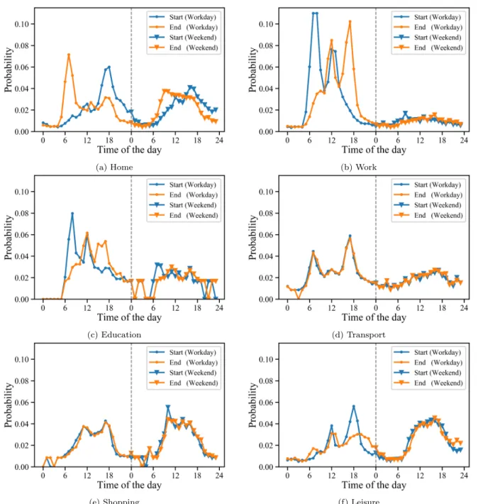
For each type of activity, the visitation probability is shown in Figure 5. The whole

327

week is divided into 48 slots. The first 24 slots are the probabilities of workdays, and

328

the last 24 slots are the visitation probabilities of weekends. All the MOBIS trips are

329

assigned to the 48 slots based on their start time and end time for all the activities.

330

The frequency of each slot is the average of the number of trips of one day. Due to

331

the mismatch between activities in the MOBIS data and POI data, we use the temporal

332

attractiveness of Shopping and Leisure in the MOBIS data as Grocery and Park in POI

333

data, respectively.

334

Based on Figure 5, we can see that the visiting probability of the start time and end

335

time varies significantly for most activities. For example, the end time of home activity

336

peaks at around 7:00 AM during the workday, while the start time of home activity peaks

337

at around 6:00 PM during the workday. Work activity displays a similar pattern during

338

workday. The peaks for the start time and end time differ remarkably during workdays.

339

These conclusions show that it is necessary to treat the origin activity and destination

340

activity differently when imputing trip purpose.

341

4.2.3. Calculating POI visit probability

342

Bayesian rule is adopted to measure the visiting probability for each candidate POI.

343

Specifically, given an origin or destination S = ((x, y ), t) and a list of candidate POIs,

344

the visit probability of candidate POI P

is defined as follows:

345

P r(P

|(x, y), t)) = P r((x, y)|P

, t)P r(P

|t)P r(t)

P r((x, y), t) (2)

Generally, the location and the time can be considered independently given P

, namely

346

P r((x, y)|P

, t) = P r((x, y)|P

), denoted as spatial attractiveness. P r(P

|t) represents an

347

activity time attractiveness. For origin, it is the probability that an activity finished at

348

the origin time. With regards to the destination, it is the probability an activity happens

349

at the end of the trip. Both P r(t) and P r((x, y), t) are constant values for a given point.

350

Thus, the visit probability can be reformulated as

351

P r(P

|(x, y), t) ∝ P r((x, y)|P

)P r(P

|t) (3)

(a) Home (b) Work

(c) Education (d) Transport

(e) Shopping (f) Leisure

Figure 5: Visitation probability for each type of activity during different hours.

4.2.4. Determining the activity type of origin and destination

352

For an origin or destination, the visit probability of all the candidate POIs can be

353

calculated following Section 4.2.3. The visit probability for each activity is denoted as

354

P r

= P

Pi∈Act

P r(P

|(x, y), t) P

Act

P

Pi∈Act

P r(P

|(x, y), t) (4) It should be noted that, instead of selecting a particular activity, the probabilities of all

355

activities are utilized to represent the activity type of the given origin or destination.

356

5. Results

357

5.1. Spatial and temporal analysis

358

5.1.1. Spatial changes on micro-mobility

359

In this section, we explore how micro-mobility patterns change over space for the three

360

types of services during the Normal and Lockdown period. The 31 postcode areas (PLZ)

361

in the study area are adopted as the primary spatial units, representing an administrative

362

division of the study area, and reflect the underlying contextual information of each sub-

363

region, such as population and land use type. Therefore, the spatial analysis focuses on

364

examining how the trip volume varies across the postcode areas during the two periods.

365

To cope with this problem, we assign the daily trip volume to the corresponding PLZ for

366

the three types of micro-mobility services respectively. Figure 6 shows the average daily

367

volume of trips by PLZ for the three types of services, which are aggregated according to

368

the drop-off points of trips. The blue and beryl green bars indicates the daily trip volume

369

in the Normal (N

) and Lockdown (N

) periods, respectively. The background color

370

represents the ratio of the daily trip volume in the Lockdown to the daily trip volume in

371

the Normal period for the three types of services (

N P

).

372

As shown in Figure 6, the three types of micro-mobility services present some simi-

373

lar patterns between Normal and Lockdown periods. First, compared with the Normal

374

period, the daily trip volume declines to varying degrees for most of the PLZs for the

375

three types of services during the Lockdown period. Especially, the significant decreases

376

are mainly concentrated in the central regions, such as PLZ 8001, 8002, 8003, and 8004,

377

and 8005, which has more Shopping, Leisure, Transport, and Work POIs compared with

378

other PLZs. In the Normal period, these POIs attract more passengers for various activi-

379

ties than other PLZs. However, during the Lockdown, most people started working from

380

home and reduced the travel to avoid coronavirus exposure. Thus, an obvious change of

381

the daily trip volume for the three types of services can be observed in central regions.

382

Second, the trip volume in some PLZs displays a slight decrease or even increase during

383

Lockdown period, such as PLZ 8046, 8051, and 8152. One possible explanation is that

384

most POIs in these PLZs are residence and the proportion of Home related activities

385

increased during the Lockdown period, as they are not influenced too much by the lock-

386

down. Third, no trips are detected within the several peripheral PLZs of the study area

387

for the three types of services, such as PLZ 8105, 8802, 8053. The main reason is that

388

there are no stations in those regions for docked bike and docked e-bike. For dockless

389

e-bike service, the reason can be the small number of e-bikes that may not be able to

390

satisfy travel demand very well over the whole study area.

391

It is worth noting that the three types of services also display dissimilarities. For

392

instance, the daily trip volume of dockless e-bike is less than those of docked e-bike

393

and docked bike. The potential explanation is that the operators provide more bicycles

394

(i.e., 797 and 859 for docked bike and docked e-bike) for the two docked services than

395

the dockless e-bike (i.e., 193) in the market. Note that even though docked bikes and

396

docked e-bikes display similar numbers of bicycles and the same docking stations, the

397

trip volume produced by docked e-bike service is remarkably higher than that of docked

398

bike by cross-referencing Figure 6a and 6b. It can be attributed to the hilly terrains in

399

Zurich. Some PLZs with a high average elevation can be 200 meters higher than the PLZ

400

with a low elevation. Thus, docked e-bikes are more attractive than docked bikes while

401

traveling. Additionally, several PLZs with low trip volume for docked bike service (e.g.,

402

PLZ 8006, 8057) have high trip volumes for docked and dockless e-bike, which further

403

demonstrate people’s preference for the e-bike, especially in those hilly regions. Moreover,

404

this preference has not been influenced by COVID-19 by comparing the trip volume in

405

those PLZs during the two periods.

406

(a) Docked bike (b) Docked e-bike

(c) Dockless e-bike

Figure 6: The spatial distribution on micro-mobility daily trip volume for different types of micro- mobility services. The blue bar and beryl green bar are the daily trip number in Normal period (N

) and Lockdown period (N

), respectively. The background color of each PLZ represents the ratio of the daily trip number in Lockdown and Normal period (

N P

) for the given PLZ.

5.1.2. Temporal changes on micro-mobility

407

The spatial analysis uncovers how micro-mobility patterns vary over space during

408

the Normal and Lockdown periods. It is necessary to evaluate the changes of micro-

409

mobility patterns in finer-grained time periods. In this section, the Normal and Lockdown

410

periods are further divided into four sub-periods: Normal workday, Normal weekend,

411

Lockdown workday, and Lockdown weekend. In each period, the micro-mobility patterns

412

are analyzed from three aspects for the three types of services, including the average

413

number of trips, trip duration, and trip distance.

414

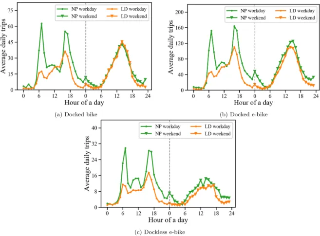
Figure 7 reveals how micro-mobility patterns change over time on an hourly basis in

415

terms of average number of trips. Some similarities and differences are observed for the

416

three types of micro-mobility services during the Normal and Lockdown period. During

417

the Normal period, it can be seen that: (1) there are two obvious peaks for the three

418

types of services, namely morning peak (6:00-8:00 AM) and evening peak (4:00-5:00 PM)

419

on workday, which match well with the commuting patterns. It denotes that the trips

420

for commuting could account for a high proportion of all the biking trips. (2) There is

421

only one peak (1:00 - 3:00 PM) for the three types of services on weekends, which is lower

422

than the two peaks during workdays. During the Lockdown period, it can be observed

423

that: (1) there are still one morning peak and evening peak on weekend, while the two

424

peaks are not so conspicuous as on Normal weekdays, especially the morning peak. It

425

suggests the decline of trip volume can be attributed to the lockdown regulation and

426

most people working from home. For those who need to go to workplaces, the time has

427

become flexible, they do not need to go working at a fixed time as before. (2) There is still

428

one weekend peak, which has no significant change. However, compared with remarkable

429

reduction of average trip volume between Normal and Lockdown workday, the average

430

trip volume on weekend has no obvious change. Especially the volume of docked bike,

431

the curve of NP workday almost coincide with the curve of LD workday. Overall, we

432

can conclude that the striking difference between the Normal and Lockdown period is

433

the travel declines in the peak hours of workdays for the three types of micro-mobility

434

services.

435

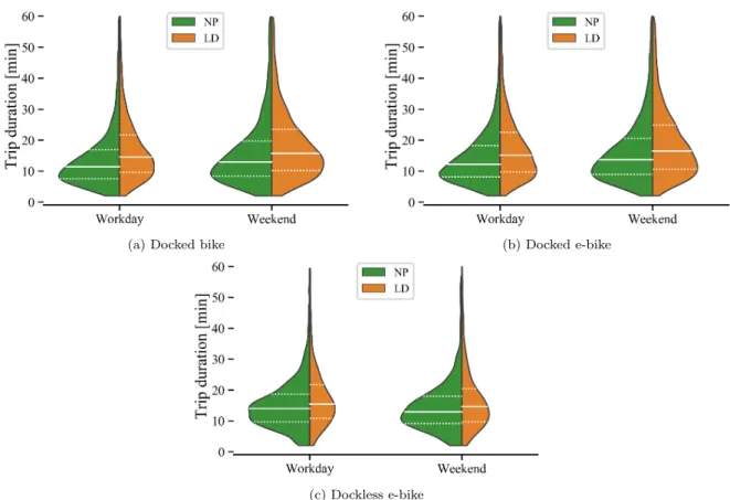
We also analyze the trip duration distribution during the four periods. For each

436

type of service, the transaction data are divided into four groups based on the sub-

437

periods. In each group, the distribution of trip duration is plotted by the violinplot

438

function of the seaborn library

, which is a combination of boxplot and kernel density

439

estimate. Furthermore, to assess the variation in the Normal period and Lockdown period

440

statistically, we employ the t-test to examine the difference between periods for each type

441

of service, as displayed in Table 4.

442

As illustrated in Figure 8, the solid white lines represent the median and the dashed

443

white lines are the quartiles. First, it can be observed that the statistics of trip duration

444

distributions on Normal workday are lower than those on Lockdown workday correspond-

445

ingly for the three types of services. Likewise, the similar conclusion can be reached on

446

Normal weekend and Lockdown weekend for the three types of services. It is demon-

447

strated that the trip duration in Lockdown period is on average higher than Normal

448

period on both workday and weekend for the three bike (e-bike) services. In addition,

449

the kernel density curve on Normal workday or weekend is shown to be taller and thinner

450

than that on corresponding Lockdown workday and weekend for the three types of ser-

451

vices. It also indicates that the proportions of trips with long duration increased during

452

Lockdown period for the micro-mobility services. We can conclude that people tend to

453

ride bike (or e-bike) for long-duration travels during the Lockdown period. One possi-

454

ble explanation is that people may need to use micro-mobility services for longer trips

455

compared with the Normal period. Also, although the trip duration distributions for the

456

4

https://seaborn.pydata.org/index.html

(a) Docked bike (b) Docked e-bike

(c) Dockless e-bike

Figure 7: Average number of trips during Normal and Lockdown periods.

micro-mobility services have changed from the Normal to the Lockdown period, these

457

changes are mainly for the trips over 20 minutes. We further apply the t-test to examine

458

whether the difference between the mean of trip duration on Normal workday (or week-

459

end) and Lockdown workday (weekend) for each type of service. As displayed in Table

460

4, all the changes in Figure 8 are significant at the 0.01 significance level.

461

Table 4: Pairwise t-test for the trip duration distribution during different periods

Period 1 Period 2 Docked bike Docked e-bike Dockless e-bike

NP LD <0.01*** <0.01*** <0.01***

NP workday LD workday <0.01*** <0.01*** <0.01***

NP weekend LD weekend <0.01*** <0.01*** <0.01***

***, **, * represents the significance at the 0.01, 0.05, 0.1 level, respectively

We further explore the trip distance distribution during the four specific periods, which

462

reflects how far users travel using micro-mobility services. In a similar manner, Figure

463

9 displays the trip distance distribution during the four sub-periods for the three types

464

of micro-mobility services. First, it is reported that the docked bikes mainly serve the

465

trips less than 2 km compared with docked and deckless e-bikes. People can ride docked

466

and dockless e-bikes for longer trips due to electric power. Second, as can be seen from

467

Figure 9, the moments of trip distance distribution on Normal workday (or weekend) are

468

also lower than those on Lockdown workday for each type of service. The trip distance in

469

Lockdown period is on average longer than Normal period on both workday and weekend

470

for the three types of services, which is in accordance with the conclusion drawn from

471

(a) Docked bike (b) Docked e-bike

(c) Dockless e-bike

Figure 8: The distribution of trip duration in each period. The curve of each patch represents kernel density estimation of trip duration. The solid white lines are median of the trip duration. The dashed white lines from bottom to top are the first and third quartile of the trip duration.

Figure 8. Third, the kernel density estimation results also illustrate that the proportions

472

of the trips more than 2 km increased during Lockdown periods. We can speculate that

473

people may choose the micro-mobility services for some of the medium- or long-distance

474

trips by replacing public transport modes (i.e., train, bus, and tram) during Lockdown.

475

Furthermore, we also examine the significance of the trip distance changes during the

476

two periods using t-tests, as shown in Table 5. The table shows that the mean of trip

477

distance has changed significantly between the Normal and Lockdown period for all the

478

three micro-mobility services.

479

Table 5: Pairwise t-test for trip distance distribution during different periods

Period 1 Period 2 Docked bike Docked e-bike Dockless e-bike

NP LD <0.01*** <0.01*** <0.01***

NP workday LD workday <0.01*** <0.01*** <0.01***

NP weekend LD weekend <0.01*** <0.01*** 0.05*

***, **, * represents the significance at the 0.01, 0.05, 0.1 level, respectively

5.2. Network construction and spatial network characteristics

480

As described in subsection 4.1 on spatially embedded network construction and spa-

481

tial network analysis, spatial interaction network can be constructed based on origin-

482

destination movement flow matrix calculated from the micro-mobility data.

483

Figure 10 displays the spatial interaction networks before and during the Lockdown

484

period for the three types of micro-mobility services. The size of red point represents the

485

(a) Docked bike (b) Docked e-bike

(c) Dockless e-bike

Figure 9: The distribution of trip length in each period. The curve of each patch represents kernel density estimates of the trip length. The solid white lines are median of the trip duration. The dashed white lines from bottom to top are the first and third quartile of the trip duration.

strength of each node, and the width of green line denotes the number of trips occurring

486

between the two corresponding nodes. For each type of micro-mobility service, the node

487

and link share the same legend scale in the two periods. First, it can be observed that

488

most links of the network become thinner during the Lockdown period for the identical

489

type of micro-mobility service. It could be attributed to the reduction of non-essential

490

travels due to the implementation of the lockdown policy in Switzerland. Second, it is

491

also found that several nodes become smaller during the Lockdown period for each type

492

of service, which implies that the numbers of connections between those PLZs and other

493

PLZs decreased compared with the Normal period. These nodes are mainly distributed

494

in the city center, such as PLZ 8001, 8002, 8003, 8004, and 8005, which contain a large

495

amount of shopping and entertainment facilities and the Zurich Main Station. Influenced

496

by the pandemic, the number of trips to city center decreased significantly due to the

497

reduction of unnecessary activities (e.g., entertainment and leisure). It should be noted

498

that although the nodes with higher degrees and the links with higher weights of the three

499

networks during the Normal period become smaller and thinner in the corresponding

500

networks during the Lockdown period, the number of nodes and links do not change

501

between the two periods. We can speculate that the micro-mobility services still play a

502

significant role in human travel during the Lockdown period even if the number of trips

503

decreased compared with the Normal period.

504

Moreover, we quantify the changes in micro-mobility patterns by calculating the net-

505

work properties, as shown in Table 6. From the table, some changes between the Normal

506

and Lockdown period can be recognized: (1) the number of nodes that represents the

507

number of PLZs served by bikes and e-bikes are identical during the periods for each type

508

(a) Docked bike (Normal) (b) Docked bike (Lockdown)

(c) Docked e-bike (Normal) (d) Docked e-bike (Lockdown)

(e) Dockless e-bike (Normal) (f) Dockless e-bike (Lockdown)

Figure 10: Network construction for the three types of micro-mobility services during the two periods.

The size of red dot represents the degree of the node. The width of green line represents the weight of

the link.

of micro-mobility service, which implies that the service areas of micro-mobility modes

509

have not been influenced by the pandemic. (2) the numbers of edges increased for the

510

docked bike and e-bike services, while decreasing for the dockless e-bike service. The

511

PLZs within the study area became more connected through intra-urban micro-mobility

512

during the Lockdown period. The causes of the increases for docked bike and e-bike

513

services are probably that some people selected the two types of micro-mobility services

514

for their travels as the substitute for public transportation. Compared with the fixed

515

stations of docked bike and e-bike within central areas, dockless e-bikes can be parked

516

almost anywhere. Considering the reduction of human travel during the Lockdown pe-

517

riod and the small number of deckless e-bikes within the study area, we speculate that

518

the decrease for dockless e-bike service could be interpreted as its low circulation during

519

the Lockdown period. For example, the e-bikes that were parked at the less populated

520

areas may be lost to the users for a long period. (3) Similarly, the increased average

521

degrees of the docked bike and e-bike networks during the Lockdown period also show

522

the higher connectivity. For example, Figure 10a, 10b and Figure 10c, 10d show that the

523

number of links to PLZ 8052 increases from the Normal period to the Lockdown period.

524

(4) The decreased average strength for the three networks during the Lockdown period

525

further quantitatively depicts the reduction of human travels by micro-mobility services.

526

(5) Given that the number of nodes is unchanged for each type of micro-service network,

527

the change of graph density is consistent with that of node edges.

528

Overall, these results suggest that the docked bike and e-bike mobility networks be-

529

came denser during the Lockdown period, while the dockless e-bike mobility network

530

became slightly sparser even if the numbers of trips decreased significantly for the three

531

types of micro-mobility services.

532

Table 6: Statistical indicators of network analysis with data in Normal and Lockdown period.

Period Number

of nodes

Number of edges

Average degree

Average strength

Graph density

Docked bike Normal 22 292 26.545 1248.45 0.63

Lockdown 22 331 30.091 794.82 0.71

Docked e-bike Normal 22 428 38.91 3702.09 0.93

Lockdown 22 437 39.73 2324.91 0.95

Dockless e-bike Normal 26 433 33.41 551.26 0.67

Lockdown 26 406 31.33 235.22 0.63

5.3. Semantic analysis for different types of trips

533

In this section, we further explore the micro-mobility changes from the perspective

534

of semantics by analyzing trip purpose (or activity type). After recognizing the activity

535

types of origin and destination for each trip, we calculate the shares of human activities

536

in each period for the three types of micro-mobility services, as displayed in Table 7.

537

Specifically, both the Origin and Destination activities are investigated respectively for

538

all the trips. In each block, the NP and LD columns represent the share of an activity

539

in Normal and Lockdown periods for the origin or destination, denoted as S

and S

,

540

respectively. The Ratio columns further quantify how the share of each activity changes

541

between the Normal and Lockdown periods, which can be calculated by (S

−S

)/S

.

542

Note that the table is ranked by the share of activities for docked bike service in the

543

Normal period.

544