High-precision atomic force microscopy withatomically-characterized tips

(1)

PAPER • OPEN ACCESS

High-precision atomic force microscopy with atomically-characterized tips

To cite this article: A Liebig et al 2020 New J. Phys. 22 063040

View the article online for updates and enhancements.

Recent citations

Quantifying the evolution of atomic interaction of a complex surface with a functionalized atomic force microscopy tip Alexander Liebig et al

-

This content was downloaded from IP address 132.199.243.31 on 30/10/2020 at 16:06

(2)

New J. Phys.22(2020) 063040 https://doi.org/10.1088/1367-2630/ab8efd

O P E N AC C E S S

R E C E I V E D

17 March 2020

R E V I S E D

27 April 2020

AC C E P T E D F O R P U B L I C AT I O N

30 April 2020

P U B L I S H E D

22 June 2020

Original content from this work may be used under the terms of the Creative Commons Attribution 4.0 licence.

Any further distribution of this work must maintain attribution to the author(s) and the title of the work, journal citation and DOI.

PAPER

High-precision atomic force microscopy with atomically-characterized tips

A Liebig , A Peronio , D Meuer, A J Weymouth and F J Giessibl

Institute of Experimental and Applied Physics, University of Regensburg, D-93040 Regensburg, Germany E-mail:alexander.liebig@ur.deandfranz.giessibl@ur.de

Keywords:atomic force microscopy, bulk insulators, electrostatic interaction, atomically-characterized tips Supplementary material for this article is availableonline

Abstract

Traditionally, atomic force microscopy (AFM) experiments are conducted at tip–sample distances where the tip strongly interacts with the surface. This increases the signal-to-noise ratio, but poses the problem of relaxations in both tip and sample that hamper the theoretical description of experimental data. Here, we employ AFM at relatively large tip–sample distances where forces are only on the piconewton and subpiconewton scale to prevent tip and sample distortions. Acquiring data relatively far from the surface requires low noise measurements. We probed the CaF

2

(111) surface with an atomically-characterized metal tip and show that the experimental data can be reproduced with an electrostatic model. By experimentally characterizing the second layer of tip atoms, we were able to reproduce the data with 99.5% accuracy. Our work links the capabilities of non-invasive imaging at large tip–sample distances and controlling the tip apex at the atomic scale.

1. Introduction

When frequency-modulation atomic force microscopy (FM-AFM) ﬁrst achieved atomic resolution, the attractive forces were on the order of 1 nN [1]. Atomic bonds in solids have typical spring constants on the order of 100 N m

⁻¹

, therefore, forces of a nanonewton stretch the bonds of surface atoms by distances on the order of 10 pm. In traditional FM-AFM, measurements are usually conducted at close tip–sample distances where the tip strongly interacts with the surface to maximize the signal-to-noise ratio. These strong tip–sample interactions can lead to lateral and vertical relaxations of the tip apex [2–7] and induce relaxations in the sample [8, 9], as had been previously investigated regarding STM experiments [10]. In particular, tip relaxation and sample perturbation have been major problems in FM-AFM studies of bulk ionic crystals, where sample relaxations greater than 100 pm were observed [11, 12]. In general, the idea of greater tip–sample distances to simplify observations and avoid perturbing the sample has far-ranging applications, from a magnetic tip changing the local spin state [13, 14] to measuring a sensitive electronic ground state [15]. These greater distances pose the challenge of acquiring data with piconewton and sub-piconewton force contrast.

Above ionic surfaces, when the tip is close to the sample, short-range chemical and van der Waals

interactions can play a dominant role in AFM images [16, 17]. At larger tip–sample separations,

electrostatic interactions have been shown to dominate the AFM contrast [16, 18] down to piconewtons

[17]. AFM experiments on bulk ionic crystals generally involve poking the tip into the sample to generate a

sharp apex, covering the AFM tip apex with a cluster of sample atoms, and therefore leaving the tip

termination and polarity unknown. Even with the assumption that the tip ends in one of the ionic species

of the surface, atomic identiﬁcation requires indirect theoretical characterization [19, 20] or adsorbed

marker molecules [21, 22]. The CaF

2

(111) surface (ﬁgures 1(A) and (B)) is an ionic surface that lacks

charge inversion symmetry and has been used for this reason to identify the charge at the tip apex [11, 12,

23– 25]. The surface layer of CaF

2

(111) consists solely of negatively charged F

⁻

ions (as otherwise, the

surface would possess an inﬁnitely high surface energy [26]).

(3)

New J. Phys.22(2020) 063040 A Liebiget al

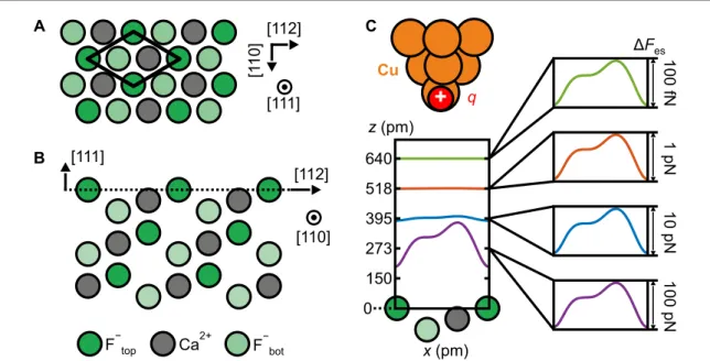
Figure 1. Schematic of the CaF2(111) surface and decay of the short-range electrostatic tip–sample interaction with distance.

(A) Top view of the CaF₂(111) surface. The surface unit cell presents three inequivalent sites, corresponding to the different ions of the topmost triple layer [26]. (B) Side view of the CaF2(111) surface. The surface layer is marked by the dashed line. (C) A single-atom metal tip has been modeled with a positive point chargeq. Graph: illustration of the exponential decay of the short-range electrostatic force contrastΔFeswith tip–sample distancezfor the single-atom metal tip above the CaF2(111) surface.

Due to the Smoluchowski effect [27], single-atom metal tips expose a dipole with its positive pole pointing toward the surface [16, 17, 28, 29], and are therefore suitable to probe ionic crystals. The apex of a metal tip can be characterized at the atomic scale by imaging a known feature to determine the chemical and structural composition of the tip apex. We use a single CO molecule on a Cu(111) surface, a technique known as the CO front atom identiﬁcation method (COFI) [30–32]. In this way, a suitable metal tip ending in a single front atom can be prepared by a sequence of poking and COFI analysis until a single atom tip is obtained. Poking and COFI requires a metal surface (typically Cu(111)) covered with a few percent of CO.

In this work we report on AFM experiments on the CaF

₂

(111) surface with a single atom metal tip which is thoroughly characterized by COFI to assess any inﬂuence of tip atoms in the second atomic layer behind the front atom. The preparation and COFI analysis of a single-atom metal tip was conducted on a Cu(111) sample, before the Cu(111) sample was replaced by the CaF

₂

(111) sample. Afterwards the tip’s state was again checked with COFI on Cu(111) (see supplementary ﬁgure S6)

(https://stacks.iop.org/NJP/22/063040/mmedia). We probed the CaF

2

(111) surface over a tip–sample distance range of 300 pm, starting with force contrasts of only 40 pN at closest approach down to femto-newtons. In this regime, the atomic AFM contrast is primarily formed due to short-range electrostatic tip–sample interactions [16]. An electrostatic calculation, where the sample atoms are represented by static point charges and the tip is modeled by a single positive point charge (ﬁgure 1(C)), reproduces the measured AFM contrast for all tip–sample distances. Figure 1(C) illustrates the electrostatic force contrast as a function of tip–sample distance: probing the surface at tip–sample distances where we measure force contrasts of only a few tens of pico-newtons down to the femto-newton regime allows us to neglect tip-induced relaxations of sample atoms in our calculation, that were previously reported for force contrasts on the order of nano-newtons [11, 12]. Based on the experimental characterization of the second layer of tip atoms, we improved the accuracy of the calculation and reproduced the small but measurable asymmetry in the images of CaF

₂

(111).

2. Experimental methods

The experiment was performed with a commercial low-temperature combined scanning tunneling/atomic force microscope at a temperature of 4.4 K (LT STM/AFM, Scienta Omicron GmbH, Taunusstein), equipped with a qPlus sensor [33]. We used a sensor with an Ir tip, sharpened with a focused-ion-beam (FIB), showing a resonance frequency of

f0=

55 051Hz, a stiffness of

k=

1800 Nm

⁻¹

, and a quality factor of

Q=

811 485, that was operated at a constant amplitude of

A=

50 pm in the frequency modulation mode (FM-AFM) [34], with a phase-locked-loop bandwidth set to

B=

50 Hz. In FM-AFM, the frequency shift

Δf

of the sensor from its unperturbed resonance frequency

f₀

is related to the gradient of the vertical

2

(4)

force between tip and sample

k_ts

as

Δf=f₀/(2k)k_ts

, where the brackets indicate a weighted average over the oscillation amplitude of the tip [35]. To increase the sensitivity to short-range tip–sample interactions, the oscillation amplitude should be set to a similar magnitude as the decay length of the tip–sample interaction [33]. As derived later in the text, the short-range electrostatic interaction on CaF

2

(111) decays exponentially with a decay length of

λtheo=

53.2 pm. Hence, we chose an amplitude of

A=

50 pm.

Processing of experimental data has been performed using the Gwyddion software [36] and is explicitly stated when applied.

A Cu(111) sample for tip preparation and characterization was prepared using standard sputter-anneal cycles and then CO was leaked into the chamber to cover the sample with 0.01 ML CO. The CaF

₂

(111) sample was cleaved in ambient conditions. It was then transferred to ultra-high vacuum and annealed several hours at about 550

^◦

C in order to remove contaminants and in contrast to previous ﬁndings [37] we did not observe atomic defects. Tips were kept cold while the samples were being exchanged to prevent thermally induced tip changes.

Single-atom metal tips were characterized and prepared on the Cu(111) sample. The tips were prepared by light pokes between 300 pm and 1 nm into a Cu(111) surface. After poking, the tip was characterized with the COFI method [30–32] and sequences of poking and COFI analysis were repeated until the tip showed a satisfactory COFI portrait. In COFI, the tip is scanned in constant height above a CO molecule adsorbed to a Cu(111) surface. The CO acts as a probe and the resulting

Δf

images show the atomic conﬁguration of the tip apex. Changes in the atomic structure of the tip apex during the measurement were excluded by investigating the tips again on Cu(111) after data was acquired of the CaF

₂

(111) surface similar to [31] (see supplementary ﬁgure S6). For direct comparison, we recorded the two corresponding COFI images at the same tip–sample distance, i.e. at the same relative distance to a given STM setpoint above the bare Cu surface. In this way we veriﬁed that the tip had not changed during the measurement on

CaF

₂

(111). We note that this procedure is experimentally challenging: ﬁrst, a Cu(111) sample is inserted into the microscope, covered by CO molecules and then used to poke and characterize the tip. Second, the Cu sample is replaced by the CaF

2

(111) sample and the measurements are conducted. As a last step, the samples are again exchanged and the tip apex is characterized by COFI on the Cu(111) sample again. If the tip suffered changes during the data acquisition, the data had to be discarded.

The sample bias

Vb

was set to minimize the long-range electrostatic contribution to the total AFM contrast. We therefore measured a Kelvin parabola and used the apex voltage as the imaging voltage

Vb

. However, the position of the apex depends on the tip–sample electrostatics, so it is slightly different for measurements performed on the three high-symmetry sites. We obtained the actual imaging voltage

V_b

by averaging the apex positions measured on the three prominent sites of the topmost CaF

₂

(111) triple layer.

For the single-atom metal tip we obtained

Vb= +5.8 V (see supplementary ﬁgure S7). The measured value

of

V_CPD

is comparable to previously reported values on CaF

₂

(111) in [23].

3. Results

Figure 2(A) shows an experimental constant-height frequency shift

Δf

image of the CaF

2

(111) surface recorded with a single-atom metal tip. The image presents three prominent sites: a local minimum (dark), a local maximum (bright) and a saddle point (intermediate). Figure 2(B) shows experimental frequency shift versus distance

Δf(z) spectra recorded on the three sites with the same tip. AsΔf

is entirely negative, the spectra show that the tip–sample interaction is attractive over the accessible

z

range. At closer distances, reversible tip relaxations occurred, indicated by an increased AFM dissipation signal. The constant-height image is recorded at the height

z_img

.

To address the contrast mechanism in ﬁgure 2(A), we compare our data to simulated data including only electrostatic interactions. We model the atoms of the sample as point charges with

q_Ca= +1.730e

and

q_F =−

0.865

e

(with

e

the elementary charge) as calculated with density functional theory [38]. Note that changing the magnitude of the ionic charges (at ﬁxed ratio 2:1 to keep charge neutrality) does not affect the interpretation of the experimental data. It can be shown that the

z-component of the electric ﬁeld decays

exponentially outside an ionic crystal with a decay length

λtheo=

1/a

^∗

, where

a^∗

is the length of the surface reciprocal primitive vector [39]. The potential

V(r) at positionr

above a crystal surface has the periodicity of the surface itself in the

x

and

y

directions. When divided in components, it can be expanded in a Fourier series as [40, 41]

V(r)=

K=0

V_K

(z) e

^iK·r=

K=0

V_K

(z) e

^iK^x^x

e

^iK^y^y

, (1)

where

K=m1a^∗₁+m2a^∗₂

is a reciprocal surface lattice vector,

m1

and

m2

are integers, and

a^∗₁

and

a^∗₂

are the

surface reciprocal primitive vectors. Outside the crystal (where no charges are present) the potential must

(5)

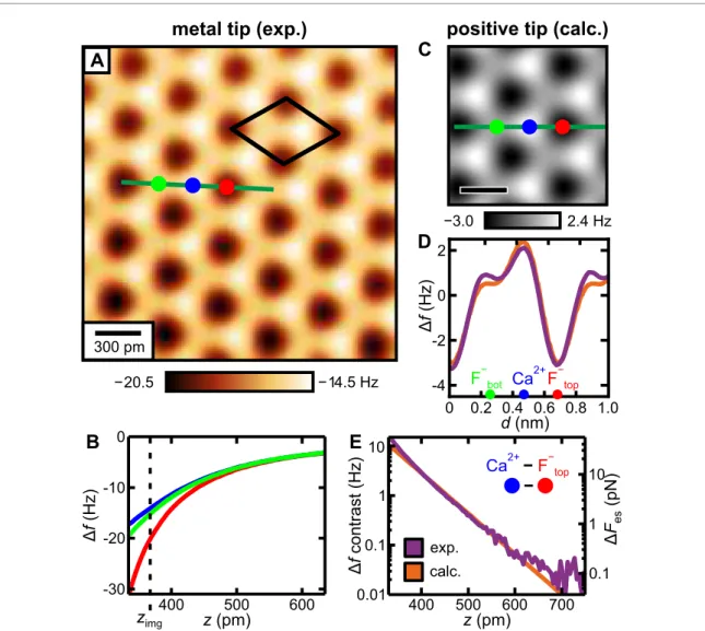
Figure 2. Experimental and calculated AFM data of CaF₂(111). (A) Experimental constant-heightΔfimage of the CaF₂(111) surface recorded with the single-atom metal tip. The unit cell deﬁned in ﬁgure1(A) is drawn black in the image. (B) ExperimentalΔf(z) curves measured with the single-atom metal tip above the three high-symmetry sites, positions marked in (A). The constant-height image in (A) has been recorded atzimg. (C) Calculated constant-heightΔfimage for a

positively-terminated tip. (D) Comparison of experimental (purple, average subtracted) and calculated (orange) line proﬁles following the respective traces in (A) and (C). (E) Comparison of experimental and calculatedΔf(z) contrasts for the metal and the positively-terminated tips, together with the electrostatic force contrastΔF_es, that was obtained from the electrostatic calculation. All scale bars are 300 pm. (A) has been processed with a 47 pm×47 pm Gaussian low-pass ﬁlter [36], to remove measurement noise before comparison between experiment and theory.

fulﬁll the Laplace equation

∇²V(r)=

0 [40]. For each

K=

0 this leads to

V_K

(z)(

−K_x²

)

+V_K

(z)(

−K_y²

)

+∂_z²V_K

(z)

=

0. (2) This differential equation can be solved by

V_K

(z)

=V_K,0

e

^−Kz=V_K,0

e

^−z/λ

, (3) where

K=

K_x²+K_y²

, and

λ=

1/K

=

1/a

^∗

. For CaF

₂

(111),

a^∗=

(4π)/(

√

3

d), whered=

386 pm is the length of the surface primitive vector, and thus

λtheo=

53.2 pm. The exponential dependence of the

z-component of the electric ﬁeld is also reﬂected in the tip–sample force and the frequency shift as the latter

two quantities are linear dependent on the effective charge at the tip apex

q

and the electric ﬁeld (see supplementary materials)

Δf

(z)

∝q

e

^−z/λ.

(4) Hence, multiplying the ionic charges with the same factor

c

would just change the measured contrast by this factor

c. This is equivalent to a change in tip–sample distance and will not alter the relative atomic contrast.

We ﬁrst calculated the electric ﬁeld above the surface, then the interaction force with a point charge

q

modeling the tip apex, and ﬁnally the frequency shift signal (described in more detail in the supplementary material). We assumed that

q= +0.13e

for a single-atom metal tip as reported in [28].

4

(6)

Figure 2(C) shows a calculated constant-height

Δf

image for the positively-terminated metal tip.

Analogous to the experimental image in ﬁgure 2(A), the calculated image shows three prominent sites that correspond to the atoms in the top triple layer of CaF

2

(111), which allows us to assign atomic species to the experimental data. The atoms of the surface F

⁻

layer are imaged dark with the metal tip and the Ca

²⁺

atoms are imaged bright in the constant-height image. The sites of intermediate contrast correspond to the atoms of the lower F

⁻

layer. Figure 2(D) shows experimental and calculated line profiles extracted along the green lines in figures 2(A) and (C), respectively. To quantify the agreement between experiment and calculation, we calculated the relative quadratic deviation (RQD) over one surface period between the measured and calculated line profiles, and define the accuracy of our calculation as 1

−

RQD (see supplementary material). In order to compare the atomic contrast and not the long-range background forces, the average

Δf

over one period is subtracted from both the experimental and calculated line proﬁles.

For the image in ﬁgure 1(A), we obtain an accuracy of 98.1% between experiment and theory, which shows that our calculation captures almost all the contrast measured in the electrostatic regime. The accuracy is increased to 99.5 % by taking the second tip layer into account (see section 3.2).

The experimental

Δf(z) curves in ﬁgure

2(B) reﬂect the total tip–sample interaction, whereas in the calculation only short-range electrostatics are taken into account. To eliminate the long-range contribution in the data we consider the difference of

Δf(z) spectra above two atomic sites, analogously to [42].

Calculated and experimental

Δf(z) contrasts are shown on a logarithmic plot in ﬁgure

2(E). For

z

values between 350 pm and 700 pm, the measured

Δf

spectra show an exponential decay with a decay constant of

λexp=

(53

±

3) pm, in agreement to the predicted electrostatic decay constant

λtheo =

53.2 pm. The

Δf(z)

contrasts shown in ﬁgure 2(E) demonstrate that the electrostatic model is sufﬁcient to explain the contrast measured with the metal tip for all accessible tip–sample distances, i.e. the short-range electrostatic

interaction dominates the AFM contrast for all accessible tip–sample distances for the single-atom metal tip [16].

We used this relationship to determine the tip height

z

in the experimental data by ﬁtting the

experimental to the calculated

Δf(z) contrast, using the tip–sample distance as a ﬁt parameter. We deﬁnez

as the vertical distance between the point charge modeling our tip and the F

⁻_top

nucleus. In this estimate, a factor of 2 uncertainty in the charge at the tip apex,

q, translates in an uncertainty inz

of only

±

37 pm (see supplementary materials). Analogous, if we change the ionic charges of the sample atoms from

qCa= +1.730e

and

qF =−0.865e

to

qCa= +2e

and

qF=−1e, this is equivalent to a change in tip–sample

distance of only 8 pm, and will therefore not affect our interpretation.

3.1. Detecting femtonewton forces

For tip–sample distances larger than 500 pm we measure

Δf

contrasts down to the mHz range, which corresponds to femtonewton electrostatic force contrasts (figure 2(E)). As illustrated in figure 3, constant-height images recorded at these distances are primarily governed by measurement noise that exceeds the expected atomic corrugation: figure 3(A) shows an unprocessed constant-height image recorded at

z=

380 pm, clearly resolving the three atomic sites of the CaF

2

(111) surface triple layer. The inset shows a part of the image, processed with a 47 pm

×

47 pm Gaussian ﬁlter, revealing the expected atomic

Δf

contrast of 4.2 Hz. The fast Fourier transformed (FFT) image (ﬁgure 3(B)) created from ﬁgure 3(A) shows six peaks that correspond to the surface reciprocal primitive vectors.

Figure 3(C) shows an unprocessed constant-height image recorded of the same spot on the surface as ﬁgure 3(A), but at a tip–sample distance of

z=

570 pm. As in this image the tip was 190 pm further away from the surface than in ﬁgure 3(A), the atomic contrast should be only 2.8% of the initial value. This corresponds to a

Δf

contrast of 118 mHz (corresponding to an electrostatic force contrast of 350 fN, as illustrated in figure 2(E)), which is masked by the measurement noise. The corresponding FFT image (figure 3(D)) still shows the six peaks that correspond to the surface reciprocal primitive vectors in the center, but with much lower intensity than figure 3(B). A detailed description of the noise sources in AFM experiments with qPlus sensors is given in [33], showing that the linear dependence of the noise on frequency (as it is the case for the FFT image in figure 3(D)) is due to detector noise. Note that the linear increase of noise with spatial frequency is only seen in the

x-direction, which is the fast scan direction, since

in the

x-direction the number of pixels scanned per second (spatial frequency) is much higher than in the y-direction. The experimental noise in AFM experiments is complex (see [33]), it has components that are

inverse with the spatial frequency (frequency drift noise), constant (‘white noise’: thermal and oscillator noise) and linear with the spatial frequency (detector noise). In our experiment, detector noise is dominant, and as a consequence, it shows up mainly in the fast scan direction (x) where it dominates the FFT image.

The inﬂuence of the detector noise contribution can be diminished by reducing the bandwidth during

measurement. After data acquisition, low-pass ﬁltering in the time domain (i.e. bandwidth reduction) can

be performed by ﬁltering the data with a Gaussian low-pass ﬁlter. Indeed, processing the constant-height

(7)

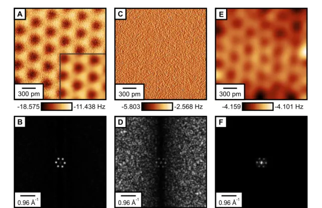
Figure 3. Experimental images with mHz contrast. (A) Experimental constant-heightΔfimage recorded at a tip–sample distance ofz=380 pm. Inset: part of the image, processed with a 47 pm×47 pm Gaussian low pass filter [36], showing aΔf contrast of 4.2 Hz. (B) Fast Fourier transformed (FFT) image created from (A) resolving six peaks that correspond to the surface reciprocal primitive vectors. (C) Experimental constant-heightΔfimage recorded at a tip–sample distance ofz=570 pm. The expected atomic contrast of only 118 mHz is masked by measurement noise. (D) Corresponding FFT image created from (C), still showing the six peaks corresponding to the reciprocal lattice, but masked by measurement noise. (E) Same image as in (C), processed with a 234 pm×234 pm Gaussian low-pass filter [36], again resolving the atomic lattice of CaF2(111). The strong features at the corners are an effect of the low-pass filtering. (F) FFT image created from (E), showing the increased signal-to-noise ratio after image processing.

image in ﬁgure 3(C) with a 234 pm

×

234 pm Gaussian ﬁlter reveals the atomically resolved CaF

₂

(111) lattice (figure 3(E)). The corresponding FFT image (figure 3(F)) shows the increased signal-to-noise ratio in the processed image with a strongly decreased contribution of detector noise and unchanged intensity of the six data peaks that correspond to the surface reciprocal primitive vectors. Note that the atomic contrast in the filtered image of 58 mHz is lower than the theoretically expected contrast of 118 mHz, which can be attributed to the strong Gaussian low-pass filtering that leads to an averaging effect, but is needed to resolve the atomic contrast in the constant-height image [33].

3.2. Improving the tip model from a single point charge to a model that takes the second tip layer into account by utilizing the COFI data

The CaF

2

(111) surface has a three-fold rotational symmetry with respect to an axis perpendicular to the surface. Experimental constant-height line proﬁles extracted along the three high-symmetry directions of the surface are shown as dotted lines (green, red and blue) in ﬁgure 4(C). The slight difference between them (e.g. the green line decreases between

d=

0.2 and 0.3 nm, whereas the blue line remains constant in this range) is a result of the fact that the actual metal tip does not perfectly share this threefold symmetry, unlike a tip comprised by a single point charge in our model.The COFI image of this tip (ﬁgure 4(A)) shows signatures of atoms in the second tip layer, as indicated by the crosses. We expanded the electrostatic model to also consider contributions from the relevant second tip layer atoms. The lateral positions (Δx

_i

,

Δy_i

) and magnitudes of the additional force contributions of the second layer tip atoms were directly obtained from the COFI portrait of the tip: from the image we obtained the lateral shift (Δx

i

,

Δyi

) of the 3 second layer atoms (black crosses in ﬁgure 4(A)) with respect to the front atom marked by the white cross.

Note that the COFI image is a mirror inverted image of the atomic structure of the tip [43]. As an example, if a feature is 200 pm left of the front atom in the COFI image, i.e. in negative

x

direction, it is 200 pm right of the front atom in real space. To calculate the magnitude of the additional contributions to the

Δf

contrast, we analyzed the signal strength in the COFI image of each second layer atom with respect to the front atom (see supplementary material for details). In this way, the COFI portrait ﬁxes all relevant tip parameters.

6

(8)

Figure 4. Refined tip apex description based on the COFI characterization. (A) COFI image of the single-atom metal tip. The white cross indicates the front atom at coordinates (0, 0). Black crosses indicate second layer atoms (shifted with respect to the front atom by (Δx_i,Δy_i)) used to refine the electrostatic calculation. Note: yellow color indicates a local minimum. (B) CalculatedΔf image of CaF2(111) for the multi-atom tip model. (C) Line profiles along the three high-symmetry directions marked in (B). The calculation including four point charges (solid) matches the asymmetry of the experiments (dots) and gives a better agreement than the single point charge model (dashed).

With the second layer atoms, we calculated again constant-height images of the CaF

₂

(111) surface (figure 4(B)). Figure 4(C) shows a comparison between experimental data (dotted), the single point charge model (black, dashed) and the calculation with second tip layer (solid). While the single point charge model cannot reproduce the asymmetry in the line profiles, taking into account the second tip layer drastically increases the agreement. The more refined model reproduces the experimental image at closest approach with an accuracy of 99.8%. Over a distance range of 100 pm, the average accuracy is 99.5% (see

supplementary material).

4. Discussion

The agreement of the simulation to the experimental data shows that static electrostatics are the dominant physics between the surface and the tip. Polarization of the tip in the electric ﬁeld of the sample would lead to a deviation in the shape of the exponential decay of (4) [18]. We calculated the additional force on the metal tip due to a polarized tip apex, but compared to the electrostatic force we found this effect to be negligible (see supplementary material). Similarly, strong tip–sample interactions could induce relaxation of either the surface or the tip, which would result in a deviation from the model. We calculated the relaxation of the surface F

⁻

ions in the electric ﬁeld of our charged tip apex, and found a relaxation of only

Δz=

1.8 pm at the closest tip–sample approach of

z=

335 pm (see supplementary material). Hence, we can neglect any tip-induced sample relaxation in our data.

In conclusion, we have shown how the interpretation of experimental AFM data beneﬁts from the

precise control of the tip apex at the atomic level on the example of the well-studied CaF

₂

(111) surface. We

probed the surface with an atomically-characterized metal tip at tip–sample distances, where the tip

interacts only weakly with the sample, and atomically resolved the surface with force contrasts in the

femtonewton-regime. Due to the non-invasive imaging of the surface at these tip–sample distances, an

(9)

electrostatic calculation completely describes the AFM contrast with the metal tip. Characterizing the tip with the COFI method before and after the measurement on CaF

₂

(111) conﬁrmed the stability of the tip apex during the whole experiment, and allowed us to experimentally access the structural and chemical composition of the AFM tip apex. With this information, we could reﬁne the theoretical description of our tip, increase the accuracy of the electrostatic calculation and reproduce experimentally observed

asymmetries in the AFM images.

The approach to describe the tip apex based on experimental characterization with COFI could be in principle transferred to more complex sample systems, where more advanced theoretical modeling is required, and furthermore is not limited to the description of metal tip apices [2, 44]. By precisely

controlling the AFM tip apex in the experiment, the theoretical description of the system can be conﬁned to only one tip model and thus, calculations can be performed much more effectively.

Acknowledgments

We thank T Preis for sharpening the Ir tip with a focused-ion-beam, A Merkel for the design of the sample holder, and F Evers, J Repp, L Patera, F Huber, J Berwanger and S Matencio for fruitful discussions. We thank J Berwanger and D Kirpal for proof-reading the manuscript. Potential conﬂict of interests: FJG holds patents for the qPlus sensor. Financial support from the Deutsche Forschungsgemeinschaft (Projects No.

CRC 1277, project A02 and GRK 1570) is gratefully acknowledged.

ORCID iDs

A Liebig

https://orcid.org/0000-0002-3208-9391

A Peronio

https://orcid.org/0000-0001-9756-5670

A J Weymouth

https://orcid.org/0000-0001-8793-9368

F J Giessibl

https://orcid.org/0000-0002-5585-1326

References

[1] Giessibl F J, Hembacher S, Bielefeldt H and Mannhart J 2000Science289422–5

[2] Sun Z, Boneschanscher M P, Swart I, Vanmaekelbergh D and Liljeroth P 2011Phys. Rev. Lett.106046104 [3] Ternes M, González C, Lutz C P, Hapala P, Giessibl F J, Jelínek P and Heinrich A J 2011Phys. Rev. Lett.106016802 [4] Gross L, Mohn F, Moll N, Schuler B, Criado A, Guitián E, Peña D, Gourdon A and Meyer G 2012Science3371326–9 [5] Weymouth A J, Hofmann T and Giessibl F J 2014Science3431120–2

[6] Hapala P, Kichin G, Wagner C, Tautz F S, Temirov R and Jelínek P 2014Phys. Rev.B90085421 [7] Moll Net al2014Nano Lett.146127–31

[8] Such B, Glatzel T, Kawai S, Meyer E, Turanský R, Brndiar J and Štich I 2012Nanotechnology23045705 [9] Ondrácek M, González C and Jelínek P 2012J. Phys.: Condens. Matter.24084003

[10] Hofer W A, Fisher A J, Wolkow R A and Grütter P 2001Phys. Rev. Lett.87236104

[11] Foster A S, Barth C, Shluger A L, Nieminen R M and Reichling M 2002Phys. Rev.B66235417

[12] Hoffmann R, Barth C, Foster A S, Shluger A L, Hug H J, Güntherodt H J, Nieminen R M and Reichling M 2005J. Am. Chem. Soc.

12717863–6

[13] Schmidt R, Schwarz A and Wiesendanger R 2012Phys. Rev.B86174402 [14] Pielmeier F and Giessibl F J 2013Phys. Rev. Lett.110266101

[15] Shapir I, Hamo A, Pecker S, Moca C P, Legeza Ö, Zarand G and Ilani S 2019Science364870–5

[16] Gross L, Schuler B, Mohn F, Moll N, Pavliˇcek N, Steurer W, Scivetti I, Kotsis K, Persson M and Meyer G 2014Phys. Rev.B90 155455

[17] Ellner M, Pavliˇcek N, Pou P, Schuler B, Moll N, Meyer G, Gross L and Peréz R 2016Nano Lett.161974–80 [18] Giessibl F J 1992Phys. Rev.B4513815–8

[19] Ruschmeier K, Schirmeisen A and Hoffmann R 2008Phys. Rev. Lett.101156102 [20] Hoffmann R, Weiner D, Schirmeisen A and Foster A S 2009Phys. Rev.B80115426

[21] Lämmle K, Trevethan T, Schwarz A, Watkins M, Shluger A and Wiesendanger R 2010Nano Lett.102965–71

[22] Teobaldi G, Lämmle K, Trevethan T, Watkins M, Schwarz A, Wiesendanger R and Shluger A L 2011Phys. Rev. Lett.106216102 [23] Barth C, Foster A S, Reichling M and Shluger A L 2001J. Phys.: Condens. Matter.132061–79

[24] Foster A S, Barth C, Shluger A L and Reichling M 2001Phys. Rev. Lett.862373–6 [25] Arai T, Gritschneder S, Tröger L and Reichling M 2010J. Vac. Sci. Technol.B281279–83 [26] Tasker P W 1979J. Phys. C: Solid State Phys.124977–84

[27] Smoluchowski R 1941Phys. Rev.60661–74

[28] Schneiderbauer M, Emmrich M, Weymouth A J and Giessibl F J 2014Phys. Rev. Lett.112166102 [29] Schulz F, Ritala J, Krejˇcí O, Seitsonen A P, Foster A S and Liljeroth P 2018ACS Nano125274–83 [30] Welker J and Giessibl F J 2012Science336444–9

[31] Welker J, Weymouth A J and Giessibl F J 2013ACS Nano77377–82 [32] Emmrich Met al2015Science348308–11

[33] Giessibl F J 2019Rev. Sci. Instrum.90011101

[34] Albrecht T R, Grütter P, Horne D and Rugar D 1991J. Appl. Phys.69668–73 [35] Giessibl F J 1997Phys. Rev.B5616010–5

8

(10)

[36] Neˇcas D and Klapetek P 2012Cent. Eur. J. Phys.10181–8

[37] Bammerlin M, Lüthi R, Meyer E, Baratoff A, Lü J, Guggisberg M, Loppacher C, Gerber C and Güntherodt H J 1998Appl. Phys.A 66S293–4

[38] Shi H, Eglitis R I and Borstel G 2005Phys. Rev.B72045109 [39] Lennard-Jones J E and Dent B M 1928Trans. Faraday Soc.2492–108

[40] Feynman R P, Leighton R B and Sands M 2010The Feynman Lectures on Physics, Volume II—Mainly Electromagnetism and Matter (New York: Basic Books)

[41] Parry D E 1975Surf. Sci.49433–40

[42] Hoffmann R, Kantorovich L N, Baratoff A, Hug H J and Güntherodt H J 2004Phys. Rev. Lett.92146103

[43] Emmrich M, Schneiderbauer M, Huber F, Weymouth A J, Okabayashi N and Giessibl F J 2015Phys. Rev. Lett.114146101 [44] Liebig A and Giessibl F J 2019Appl. Phys. Lett.114143103