Assessment of upper tropospheric and stratospheric water vapor and ozone in reanalyses as part of S-RIP

(1)

https://doi.org/10.5194/acp-17-12743-2017

Assessment of upper tropospheric and stratospheric water vapor and ozone in reanalyses as part of S-RIP

Sean M. Davis^1,2, Michaela I. Hegglin³, Masatomo Fujiwara⁴, Rossana Dragani⁵, Yayoi Harada⁶,

Chiaki Kobayashi^6,7, Craig Long⁸, Gloria L. Manney^9,10, Eric R. Nash¹¹, Gerald L. Potter¹², Susann Tegtmeier¹³, Tao Wang¹⁴, Krzysztof Wargan^11,15, and Jonathon S. Wright¹⁶

1Earth System Research Laboratory, National Oceanic and Atmospheric Administration, Boulder, CO 80305, USA

2Cooperative Institute for Research in Environmental Sciences (CIRES), University of Colorado at Boulder, Boulder, CO 80309, USA

3Department of Meteorology, University of Reading, Reading, RG6 6BX, UK

4Faculty of Environmental Earth Science, Hokkaido University, Sapporo 060-0810, Japan

5European Centre for Medium-Range Weather Forecasts, Reading, RG2 9AX, UK

6Japan Meteorological Agency, Tokyo, 100-8122, Japan

7Climate Research Department, Meteorological Research Institute, JMA, Tsukuba, 305-0052, Japan

8Climate Prediction Center, National Centers for Environmental Prediction, National Oceanic and Atmospheric Administration, College Park, MD 20740, USA

9NorthWest Research Associates, Socorro, NM 87801, USA

10Department of Physics, New Mexico Institute of Mining and Technology, Socorro, NM 87801, USA

11Science Systems and Applications, Inc., Lanham, MD 20706, USA

12NASA Center for Climate Simulation, Code 606.2, NASA Goddard Space Flight Center, Greenbelt, MD 20771, USA

13GEOMAR Helmholtz Centre for Ocean Research Kiel, Kiel, 24105, Germany

14NASA Jet Propulsion Laboratory/California Institute of Technology, Pasadena, CA 91109, USA

15Global Modeling and Assimilation Office, Code 610.1, NASA Goddard Space Flight Center, Greenbelt, MD 20771, USA

16Department of Earth System Science, Tsinghua University, Beijing, 100084, China Correspondence to:Sean M. Davis (sean.m.davis@noaa.gov)

Received: 26 April 2017 – Discussion started: 23 May 2017

Revised: 23 August 2017 – Accepted: 11 September 2017 – Published: 26 October 2017

Abstract. Reanalysis data sets are widely used to understand atmospheric processes and past variability, and are of- ten used to stand in as “observations” for comparisons with climate model output. Because of the central role of water vapor (WV) and ozone (O₃) in climate change, it is important to understand how accurately and consistently these species are represented in existing global reanalyses. In this paper, we present the results of WV and O3intercomparisons that have been performed as part of the SPARC (Stratosphere–

troposphere Processes and their Role in Climate) Reanalysis Intercomparison Project (S-RIP). The comparisons cover a range of timescales and evaluate both inter-reanalysis and observation-reanalysis differences. We also provide a sys- tematic documentation of the treatment of WV and O₃ in

current reanalyses to aid future research and guide the interpretation of differences amongst reanalysis fields.

The assimilation of total column ozone (TCO) observations in newer reanalyses results in realistic representations of TCO in reanalyses except when data coverage is lacking, such as during polar night. The vertical distribution of ozone is also relatively well represented in the stratosphere in reanalyses, particularly given the relatively weak constraints on ozone vertical structure provided by most assimilated observations and the simplistic representations of ozone photochemical processes in most of the reanalysis forecast mod- els. However, significant biases in the vertical distribution of ozone are found in the upper troposphere and lower stratosphere in all reanalyses.

(2)

In contrast to O3, reanalysis estimates of stratospheric WV are not directly constrained by assimilated data. Observa- tions of atmospheric humidity are typically used only in the troposphere, below a specified vertical level at or near the tropopause. The fidelity of reanalysis stratospheric WV products is therefore mainly dependent on the reanalyses’ representation of the physical drivers that influence stratospheric WV, such as temperatures in the tropical tropopause layer, methane oxidation, and the stratospheric overturning circulation. The lack of assimilated observations and known defi- ciencies in the representation of stratospheric transport in reanalyses result in much poorer agreement amongst observational and reanalysis estimates of stratospheric WV. Hence, stratospheric WV products from the current generation of reanalyses should generally not be used in scientific studies.

1 Introduction

Ozone and water vapor are trace gases of fundamental im- portance to the radiative budget of the stratosphere. Because of their impact on stratospheric temperatures, winds, and the circulation (e.g., Dee et al., 2011), ozone and water vapor are represented as prognostic variables in almost all current reanalysis systems. However, the degree of sophistica- tion to which ozone and water vapor fields and their variability are represented depends on the reanalysis system, which observations it assimilates, which microphysical and chemical parameterizations it includes, and how those parameterizations affect the trace gas distributions. The accuracy and consistency of analysis and reanalysis ozone and water vapor fields in the upper troposphere and stratosphere has only been addressed for a limited subset of diagnostics and analysis/reanalysis systems by a few studies (e.g., Dessler and Davis, 2010; Jiang et al., 2015; Geer et al., 2006; Thornton et al., 2009).

As part of the SPARC (Stratosphere–troposphere Pro- cesses and their Role in Climate) Reanalysis Intercompari- son Project (S-RIP), we conducted the first comprehensive assessment of how realistically and consistently reanalyses represent water vapor and ozone in the upper troposphere and stratosphere. In particular, the goals of this paper are to (1) provide a comprehensive overview of how ozone and water vapor are treated in reanalyses, (2) evaluate the accuracy of ozone and water vapor in reanalyses against both assimilated and independent (non-assimilated) observations, and (3) provide guidance to the community regarding the proper usage and limitations of reanalysis ozone and water vapor fields in the upper troposphere and stratosphere.

Towards this end, in the next section, we provide a description of how ozone and water vapor are treated by the various reanalyses to provide context for the comparisons presented in the rest of the paper. We then provide an overview of the observational data sets used for comparison to reanalyses in

Sect. 3. Sections 4 and 5 contain the evaluations of reanalysis ozone and water vapor, respectively. In the final section, we conclude with a summary of the salient findings and guidance regarding the overall utility and limitations of reanalysis ozone and water vapor.

2 Description of ozone and water vapor in reanalyses In this section, we provide information on how ozone and water vapor are represented in reanalyses. The information compiled here expands on that provided by Fujiwara et al. (2017), who presented a comprehensive overview of the reanalysis systems and their assimilated observations, including a basic discussion of the treatment of ozone and water vapor.

In most reanalyses, ozone and water vapor are prognostic variables that are affected by the assimilated observations (see Tables 1 and 2 for an overview of key aspects of these fields). The assimilated observations affecting the water vapor fields in reanalyses include some combination of radiosonde humidity profiles, GNSS-RO bending angles, and either radiances or retrievals from satellite microwave and infrared sounders such as TOVS, ATOVS, and SSM/I (see Ap- pendix A for a list of all abbreviations). These observational data affect the reanalysis water vapor fields in the lower atmosphere, but radiosonde humidity data are not assimilated above a specified level in the upper troposphere (typically between 300 and 100 hPa; see Table 2). Even though radiosonde humidity data may not be assimilated above a certain level, analysis increments are possible at higher levels unless the vertical correlations of the background errors are set to zero. Where relevant, this cutoff level above which analysis increments are disallowed has been noted in Table 2.

Because stratospheric water vapor data are not directly assimilated, the treatment of water vapor in the stratosphere is highly variable amongst the reanalyses. For the modern reanalyses, the concentration of water vapor entering the stratosphere is typically controlled by transport and dehydration processes occurring in the forecast model, primarily in the tropical tropopause layer (TTL). Higher in the stratosphere, chemical production of water vapor through methane oxidation is parameterized in some reanalyses, while others use a simple relaxation of the simulated water vapor field to an observed climatology.

As with water vapor, the treatment of ozone is quite different from reanalysis to reanalysis. The ozone treatment in reanalyses (see Table 1) ranges from using prescribed ozone and a climatology in the radiation calculations (NCEP R1/R2), to using a fully prognostic field with parameterized photochemistry that interacts with the radiation calculation (CFSR, ERA-40, ERA-I, MERRA, MERRA-2), to assimilating ozone with an offline chemical transport model for use in the forecast model radiation calculation (JRA-25, JRA-55).

(3)

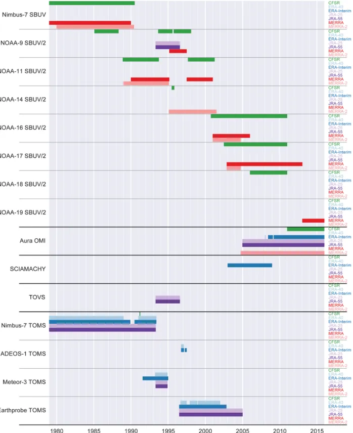
Figure 1.Total column ozone data by instrument as assimilated by the different reanalyses.

(4)

Table 1.Key characteristics of ozone treatment in reanalyses.

Reanalysis Primary TCO Vertical profile Stratospheric O₃ Stratospheric Photochemical data sources data sources used in radiative O₃treatment parameterization

transfer

NCEP R1 None None Climatology None None

NCEP R2 None None Climatology None None

CFSR SBUV SBUV Analyzed Prognostic CHEM2D-OPP

ERA-40 TOMS SBUV Climatology Prognostic CD86

ERA-I Same as ERA-40 SBUV, GOME, Same as ERA-40 Same as ERA-40 Same as ERA-40 MLS, MIPAS

JRA-25 TOMS (1979–2004)^∗ Nudging to Daily values Daily values Shibata et al. (2005) OMI (2004–) climatological from offline from offline

profile CTM CTM

JRA-55 Same as JRA-25 None Daily values Daily values Shibata et al. (2005) from updated from updated

offline CTM offline CTM

MERRA SBUV SBUV Analyzed Prognostic Stajner et al. (2008)

MERRA-2 SBUV (1980–9/2004) SBUV, MLS Same as MERRA Same as MERRA Same as MERRA OMI (9/2004–)

∗Offline CCM nudged to TOMS/OMI data.

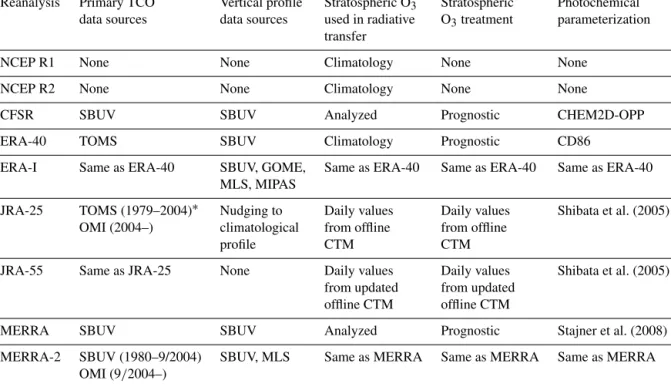
The primary ozone observations assimilated by reanalyses are satellite nadir UV backscatter-based retrievals of vertically integrated total column ozone (TCO) or broad vertically weighted averages (e.g., SBUV data). These data come from a variety of satellites that have flown since the late 1970s, and reanalyses vary widely in what subset of the available data they assimilate (Figs. 1 and 2). Some further differences exist amongst the reanalyses in their usage of different data versions from the same satellite instrument, and from different applications of data quality control and filtering. These differences in usage of input data may affect the reanalysis ozone fields.

Additional observation types using spectral ranges out- side of the UV (namely microwave and IR) and exploiting different viewing geometries (such as limb-sounding) have been used, particularly by the newest reanalyses (ERA-I, MERRA-2). The assimilation of additional data, particularly vertically resolved data, should improve the quality of the ozone in reanalyses. However, the assimilation of new data sets could introduce sudden changes in the reanalysis ozone fields, and these transition times should be considered care- fully when deriving or analyzing long-term trends.

2.1 NCEP-NCAR (R1) and NCEP-DOE (R2)

Neither NCEP-NCAR (R1) nor NCEP-DOE (R2) assimilates ozone data (Kalnay et al., 1996; Kanamitsu et al., 2002;

Kistler et al., 2001). A climatology of ozone was used for radiation calculations.

Humidity information from satellites is not assimilated in R1 and R2 (Ebisuzaki and Zhang, 2011). In general, the treatment of water vapor is similar in R1 and R2, with only a few differences. One major difference is that humidity is not output above 300 hPa in R1, whereas it is output up to 10 hPa in R2. Another difference is that only relative humidity is output in R2, whereas in R1 both specific humidity and relative humidity are output. It is worth noting that in R1, specific humidity is a diagnostics variable, computed from relative humidity and temperature. Several fixes and changes were made in the treatment of clouds in R2, and these result in R2 being∼20 % drier than R1 in the tropics at 300 hPa (Kana- mitsu et al., 2002). As the focus here is on upper levels, we do not assess humidity fields from R1 or R2. It is worth noting that R1 shows negative long-term humidity trends between 500 and 300 hPa (Paltridge et al., 2009); however, these negative trends appear to reflect suspect radiosonde measurements at these levels and are not found in other reanalyses or satellite data (Dessler and Davis, 2010).

2.2 CFSR

The Climate Forecast System Reanalysis (CFSR) is a newer NCEP product following the NCEP R1 and R2 reanalyses but with numerous improvements (see Saha et al., 2010, for details), including an updated forecast model and data as-

(5)

Table 2.Key characteristics of water vapor treatment in reanalyses.

Reanalysis Assimilation Highest level Highest level Stratospheric Stratospheric Stratospheric of satellite of assimilated of analyzed WV used in WV treatment methane

humidity WV observations WV¹ radiative oxidation

radiances? transfer parameterization?

NCEP R1 No 300 hPa 300 hPa Climatology None No

NCEP R2 No 300 hPa 10 hPa Climatology None No

(RH only)

CFSR Yes 250 hPa None Analyzed; negative Prognostic No

values set to 0.1 ppmv

ERA-40 Yes Diagnosed tropopause. Diagnosed Analyzed Prognostic Yes. Relaxation

Radiosonde humidity tropopause to 6 ppmv WV

generally used to 300 hPa at stratopause

ERA-I Yes Same as ERA-40 Diagnosed Analyzed Prognostic Yes. Relaxation

tropopause to 6.8 ppmv WV

at stratopause

JRA-25 Yes 100 hPa 50 hPa Constant 2.5 ppmv Prognostic² No

JRA-55 Yes 100 hPa 5 hPa Climatological Prognostic² No

annual mean from HALOE and UARS MLS during 1991–1997

MERRA Yes 300 hPa None Analyzed 3-day relaxation No

to zonal mean monthly mean satellite-based climatology

MERRA-2 Yes 300 hPa None Same as MERRA Same as MERRA No

1Level above which assimilation-related increments are not allowed.

2Water vapor not provided above 100 hPa in pressure level analysis products.

similation system. CFSR was originally provided through the end of 2009, but output from the same analysis system was extended through the end of 2010 before transitioning to the CFSv2 analysis system starting in January 2011 (Saha et al., 2014). Because CFSv2 was intended as a continuation of CFSR, in this paper we refer to both CFSR (i.e., CFSRv1) and CFSv2 as CFSR. However, the system changeover did result in a discontinuity in the water vapor fields that is addressed later in this paper.

CFSR treats ozone as a prognostic variable that is analyzed and transported by the forecast model. The CFSR forecast model uses analyzed ozone data for radiation calculations. In the forecast model, ozone chemistry is parameterized using production and loss terms generated by the NRL CHEM2D-OPP (McCormack et al., 2006). These production and loss rates are provided as monthly mean zonal means, and are a function of local ozone concentration. The rates do not include the coefficients for temperature and overhead ozone column provided by McCormack et al. (2006), nor heterogeneous chemistry, although late 20th century levels of CFCs are used indirectly because CHEM2D-OPP is based on the CHEM2D middle atmospheric photochemical trans-

port model, which includes ODS levels representative of the late 20th century.

CFSR assimilates version-8 SBUV profiles and TCO retrievals (Flynn et al., 2009) fromNimbus-7and SBUV/2 profiles and TCO retrievals from NOAA-9,-11, -14, -16,-17, -18, and eventually NOAA-19 (Figs. 1 and 2). The ozone layer and TCO values assimilated by CFSR have not been adjusted to account for biases from one satellite to the next, although the use of SBUV version 8 is expected to minimize satellite-to-satellite differences. Despite the fact that CFSR assimilates TCO retrievals and SBUV ozone profiles, differences have been found between CFSR and SBUV(/2) ozone profile data (Saha et al., 2010). Most of these differences are located above 10 hPa, and appear to result from observational background errors that were set too high in the CFSR upper stratosphere by between a factor of 2 (at 10 hPa) and a factor of 60 (at 0.2 hPa). Because of this, assimilated SBUV(/2) ozone layer observations do not alter the CFSR first guess for pressures less than 10 hPa, and the model first guess is used instead. The observational background errors were fixed for CFSv2, starting in 2011.

(6)

Figure 2.Ozone vertical profile observations by instrument as assimilated by the different reanalyses.

Water vapor is treated prognostically in CFSR. There are several assimilated observation types that influence the analysis humidity fields in the troposphere, including GNSS-RO bending angles, radiosondes, and satellite radiances. How- ever, as radiosonde humidity data are only assimilated at 250 hPa and greater pressures, there are no specific observations that constrain humidity in the stratosphere. Strato- spheric humidity in CFSR is hence primarily governed by physical processes and parameterizations in the model, including dehydration within the TTL. The treatment of water vapor in the model can lead to negative water vapor values around and above the tropopause. These negative values are replaced by small positive values of 0.1 parts per million by volume (ppmv) for the radiation calculations, but are retained in the analysis products. CFSR does not include a parameterization of methane oxidation.

2.3 ERA-40

The ERA-40 forecast model included prognostic ozone and a parameterization of photochemical sources and sinks of ozone, as described by Dethof and Hólm (2004). This parameterization of ozone production/loss rates is an updated version of the one proposed by Cariolle and Deque (1986, hereinafter CD86). In CD86, the net ozone production rate is parameterized as a function of the perturbation (relative to climatology) of the local ozone concentration, the local temperature, and the column ozone overhead. Compared to the CD86 formulation, the ozone parameterization in ERA- 40 includes an additional term representing heterogeneous chemistry. This loss term scales with the product of the local ozone concentration and the square of the equivalent chlo- rine concentration, and is only turned on at temperatures below 195 K. The climatologies and coefficients used in the parameterization are derived from a photochemical model and vary by latitude, pressure, and month. The prescribed chlo-

(7)

rine loading varies from year to year, from ∼700 parts per trillion (ppt) in 1950 to∼3400 ppt in the 1990s. Instead of the CD86 ozone photochemical equilibrium values, ERA-40 made use of the Fortuin and Langematz (1995) ozone climatology.

The prognostic ozone was not used in the radiation calculations, which instead assumed the climatological ozone distribution reported by Fortuin and Langematz (1995). This choice was motivated by concerns that ozone–temperature feedbacks would degrade the temperature analysis if the assimilated ozone observations were of poorer quality than the temperature observations (Dethof and Hólm, 2004).

ERA-40 assimilated TOMS TCO and SBUV layer ozone retrievals from the end of 1978 onward (Figs. 1 and 2;

see also Table 1, Dethof and Hólm, 2004; Poli, 2010). No ozonesonde measurements were assimilated, and no ozone data at all were assimilated before 1978. Ozone data prior to 1978 are thus primarily products of the photochemical parameterization. In addition, no ozone data were assimilated during 1989 and 1990 because the execution of the first ERA- 40 stream (1989–2002) was started before the ozone assimilation scheme was implemented. Ozone background errors were also changed, such that the period from January 1991 to October 1996 used different background errors than the rest of ERA-40 (Dethof and Hólm, 2004).

ERA-40 water vapor products below the diagnosed tropopause are substantially affected by assimilated observations. Three main periods can be identified (Uppala et al., 2005): until 1973, ERA-40 used only conventional in situ surface and radiosonde measurements; from 1973, satellite radiances from VTPR (1973–1978) and the TOVS instruments MSU, SSU, and HIRS (1978–onwards) were used in addition to these conventional data sources; and from 1987, 1D-Var retrievals of TCWV from SSM/I radiances were added to the assimilation. Radiosonde humidity measurements were generally used at pressures greater than 300 hPa. No adjustments to the humidity field due to data assimilation were made in ERA-40 above the diagnosed tropopause. Thus, stratospheric water vapor in ERA-40 re- flects TTL dehydration, transport, and methane oxidation.

The latter was included via a simple stratospheric parameterization, in which WV was gradually relaxed to 6 ppmv at the stratopause (Untch et al., 1998). This relaxation was later found to produce too low WV concentrations at the stratopause as it was based on earlier studies when atmospheric methane levels were lower (Uppala et al., 2005).

ERA-40 stratospheric humidity has also been shown to be too low overall, due primarily to a cold bias in TTL temperatures caused by an excessively strong Brewer–Dobson circulation (Oikonomou and O’Neill, 2006).

2.4 ERA-Interim

The treatment of ozone and water vapor in ERA-Interim is very similar to that in ERA-40. Notable differences include

additional assimilated data sets and an improved treatment of water vapor in the upper troposphere and lower stratosphere (UTLS). Descriptions of the ozone system and assessments of its quality have been provided by Dee et al. (2011) and Dragani (2011).

As with ERA-40, total ozone from TOMS (Jan- uary 1979–November 1989; June 1990–December 1994;

June 1996–December 2001) and ozone layer averages from SBUV (1979–present) are assimilated (Figs. 1 and 2). ERA-Interim also assimilates TCO from OMI (June 2008–January 2009, March 2009–present) and SCIA- MACHY (January 2003–December 2008), and ozone profiles from GOME (January 1996–December 2002), MI- PAS (January 2003–March 2004), and MLS (January–

November 2008, June 2009–present). A change in the assimilation of SBUV ozone profiles was implemented in Jan- uary 2008. Before January 2008, assimilated SBUV profiles were low vertical resolution products derived over six vertical layers (0.1–1 hPa, 1–2 hPa, 2–4 hPa, 4–8 hPa, 8–16 hPa, and 16 hPa–surface) from NOAA version 6 (v6) retrievals.

These data were replaced by native 21-vertical-level SBUV profiles from v8 retrievals. The assimilation of ozone profile retrievals from Aura MLS started in 2008 (Fig. 2) using the reprocessed v2.2 MLS retrievals and carried on with the near-real-time v3 product from June 2009 onwards.

The ozone forecast model used in ERA-Interim has the same basic formulation as that used in ERA-40, but some aspects of the parameterization have been upgraded substantially, especially the regression coefficients. An account of the changes is provided by Cariolle and Teyssédre (2007).

As in ERA-40, the radiation scheme in ERA-Interim does not use the prognostic ozone field.

A preliminary assessment of the temperature and wind fields revealed unrealistic temperature and horizontal wind increments generated near the stratopause by the 4D-Var assimilation scheme in an attempt to accommodate large local adjustments in ozone concentrations (Dee, 2008; Dra- gani, 2011). As an ozone bias correction was not available in ERA-Interim to limit the detrimental effect of ozone assimilation on temperature and wind fields, the sensitivity of the latter to ozone changes was switched off in ERA-Interim.

This change affected the period from 1 February 1996 onwards and the 10 years from 1979 through 1988 that were run at a later stage.

Through December 1995, ERA-Interim ozone analyses perform better than their ERA-40 counterparts with respect to independent ozone observations in the upper troposphere and lower stratosphere, but perform slightly worse on average in the middle stratosphere (Dee et al., 2011).

The assimilation of GOME ozone profiles (January 1996–

December 2002) improves the agreement between ERA- Interim analyses and independent data, such that ERA- Interim outperforms ERA-40 throughout the atmosphere (including the middle stratosphere) from January 1996 through the end of ERA-40 in September 2002 (Dragani, 2011).

(8)

The ERA-Interim humidity analysis is substantially mod- ified from that in ERA-40 due to changes in both model physics and assimilated observations. A non-linear transfor- mation of the humidity control variable was introduced to make humidity background errors more Gaussian (Uppala et al., 2005; Hólm, 2003; Hólm et al., 2002). This transforma- tion normalizes relative humidity increments by a factor that depends on background estimates of relative humidity and vertical level. A 1D-Var assimilation of rain-affected radiances over oceans was also added as part of the 4D-Var outer loop (Dee et al., 2011), which helps to constrain the spatial distribution of total column water vapor (TCWV). The ERA- Interim humidity analysis also benefits from several changes in the model physics, including changes in the convection scheme that lead to increased convective precipitation (particularly at night), reduced tropical wind errors, and a better representation of the diurnal phasing of precipitation events (Bechtold et al., 2004). The non-convective cloud scheme has also been updated.

Perhaps of most relevance for humidity in the UTLS, the revised cloud scheme contains a new parameterization that allows supersaturation with respect to ice in the cloud- free portions of grid cells with temperatures less than 250 K (Tompkins et al., 2007). The inclusion of this parameterization results in substantial increases in relative humidity in the upper troposphere and in the stratospheric polar cap relative to ERA-40 (Dee et al., 2011). Methane oxidation in the stratosphere is included via a parameterization like the one used in ERA-40 but with relaxation to 6.8 ppmv at the stratopause (rather than 6 ppmv as in ERA-40), based on an analysis of UARS data by Randel et al. (1998).

As with ERA-40, no adjustments due to data assimilation are applied in the stratosphere (above the diagnosed tropopause). ERA-Interim tropospheric humidity is affected by the assimilation of radiosonde humidity measurements, radiances from the TOVS (through 5 September 2006) and ATOVS (from August 1998) instrument suites, and TCWV retrievals based on rain-affected radiances from SSM/I (from August 1987). Recent ERA-Interim humidity analyses may also be affected by the assimilation of GNSS-RO bending angles (from May 2001) and/or AIRS all-sky radiances (from April 2004).

2.5 JRA-25 and JRA-55

Ozone observations were not assimilated directly in the JRA- 25 and JRA-55 systems (Kobayashi et al., 2015; Onogi et al., 2007). Instead, daily three-dimensional ozone fields were produced separately and provided to the JRA forecast model (i.e., to the radiation scheme). Daily ozone fields in JRA-55 for 1978 and earlier are interpolated in time from a monthly mean climatology for 1980–1984. Daily ozone fields in both systems for 1979 and later are produced using an offline chemistry climate model (MRI-CCM1, Shibata et al., 2005) that assimilated satellite observations of TCO us-

ing a nudging scheme. Assimilated TCO retrievals are taken from TOMS on Nimbus-7 and other satellites for the period 1979–2004 and from Aura OMI after the beginning of 2005.

Different versions of MRI-CCM1 and different preparations of the ozone fields have been used for JRA-25 and JRA- 55. For JRA-25, MRI-CCM1 output was also nudged to climatological ozone vertical profiles to account for a known bias in tropospheric ozone that produces a bias in stratospheric ozone after nudging to observations of total ozone.

This procedure produced reasonable peak ozone-layer values in the final ozone product. This vertical-profile nudging was not necessary for JRA-55, which used an updated version of MRI-CCM1. JRA-55 produces improved peak values in vertical ozone profiles relative to JRA-25, as well as a clear ozone quasi-biennial oscillation (QBO) signature.

As with other modern reanalyses, JRA-25 and JRA-55 humidity fields are affected by the assimilation of radiosonde humidity measurements and satellite radiances. The JRA- 25 assimilation analyzed the logarithm of specific humidity (Onogi et al., 2007). Stratospheric humidity was dry-biased and generally decreased with time in JRA-25, in part due to the lack of parameterized methane oxidation. The JRA- 25 forecast model radiation calculations assumed a constant value of 2.5 ppmv in the stratosphere. Water vapor in the UTLS shows evidence of discontinuities at the start of 1991, which corresponds to the transition between the two major processing streams of JRA-25. Onogi et al. (2007) reported sudden jumps of+0.7 ppmv at 150 hPa and +0.9 ppmv at 100 hPa associated with this transition.

The treatment of water vapor in JRA-55 is similar in most respects to that in JRA-25. JRA-55 does not contain a parameterization of methane oxidation. Differences include a change in the upper boundary above which the vertical correlations of humidity background errors are set to zero, pre- venting spurious analysis increments at higher levels. This boundary is set at 5 hPa in JRA-55, relative to 50 hPa in JRA- 25. Forecast model radiation calculations in JRA-55 use an annual mean climatology of stratospheric water vapor derived from UARS HALOE and UARS MLS measurements made during 1991–1997 in the stratosphere, rather than the constant 2.5 ppmv used in JRA-25. The introduction of an improved radiation scheme in JRA-55 greatly reduced lower stratospheric negative temperature biases that were present in JRA-25 during the TOVS period before 1998 (Kobayashi et al., 2015; Fujiwara et al., 2017), which may have beneficial impacts on JRA-55 stratospheric humidity products by impacting dehydration in the TTL. However, water vapor concentrations at pressures less than 100 hPa are not provided in the standard pressure-level products of these two reanalyses (although these concentrations are provided in model-level products), and are therefore not evaluated in this paper.

(9)

2.6 MERRA

Ozone is a prognostic variable in MERRA, and is subjected to assimilation, transport by assimilated winds (more pre- cisely, the odd-oxygen family is the transported species), and parameterized chemistry. The MERRA general circulation model (GCM) uses a simple chemistry scheme that ap- plies monthly zonal mean ozone production and loss rates derived from a two-dimensional chemistry model (Stajner et al., 2008). Ozone data assimilated in the reanalysis include partial columns and total ozone (defined as the sum of layer values in a profile) from a series of SBUV instruments (Flynn et al., 2009) on various NOAA platforms (Figs. 1 and 2). Version 8 of the SBUV retrievals (Flynn, 2007) is used but the native 21 vertical layers are combined into 12 layers (each 5 km deep) prior to assimilation. All other assimilated data, including radiance observations, are explicitly prevented from impacting the ozone analysis directly.

Since SBUV sensors measure backscatter solar ultraviolet radiation, only daytime observations are available; wintertime ozone in polar regions is thus poorly constrained by observations. Early NOAA satellites experienced orbital drifts that resulted in reduced daylight coverage over time. For example, the equatorial crossing time for NOAA-11 drifted from

∼2 pm in 1989 to ∼5 pm 5 years later, leading to limited SBUV coverage in 1994 (ozone observations were entirely unavailable south of 30^◦S during that austral winter). A similar orbital drift in the NOAA-17 satellite impacted the quality of the MERRA ozone products in 2012 before the introduction of observations from NOAA-19 SBUV in 2013. Out- side of the exceptions described above and occasional short temporal gaps, SBUV provides good coverage of the sunlit atmosphere.

Background error SDs for ozone are specified as∼4 % of the global mean ozone on a given model level. Horizontal background error correlation lengths vary from∼400 km in the troposphere to∼800 km at the model top. Assimilated ozone fields are fed into the forecast model radiation scheme and are used in the radiative transfer model for radiance assimilation.

Water vapor is also a prognostic assimilated variable in MERRA; however, unlike ozone, moisture fields in the stratosphere are relaxed to a 2-D monthly climatology with a relaxation time of 3 days. This climatology is derived from water vapor observations made by the UARS HALOE and Aura MLS instruments (e.g., Rienecker et al., 2011, and references therein). This climatological constraint is introduced gradually over the layer between the model tropopause and 50 hPa, where pressure-dependent blending between the climatology and the GCM water vapor is applied. Water vapor above the tropopause does not undergo physically meaning- ful variations on timescales longer than the 3-day relaxation timescale except in the lowermost stratosphere where the climatology is given a smaller weight. No attempt was made

to account for methane oxidation or trends in stratospheric methane concentrations.

MERRA assimilates specific humidity measurements from radiosondes at pressures above 300 hPa and marine surface observations. Moisture fields are affected by microwave radiance data from SSM/I and AMSU-B/MHS, infrared radiances from HIRS, the GOES Sounder, and AIRS, and rain rates derived from TMI and SSM/I. Background error statis- tics for water vapor were derived using the National Meteo- rological Center method and applied using a recursive filters methodology (Wu et al., 2002). The moisture control variable is pseudo-relative humidity (Dee and Da Silva, 2003).

2.7 MERRA-2

The key differences between the treatment of ozone in MERRA-2 (Gelaro et al., 2017) and that in MERRA are in the observing system and background error covariances.

From January 1980 to September 2004, MERRA-2 assimilates v8.6 SBUV retrievals of partial columns on a 21-layer vertical grid (Bhartia et al., 2013) and total ozone computed as the sum of individual layer values. Compared to the v8 retrievals used in MERRA, the v8.6 algorithm uses upgraded ozone cross sections and an improved cloud height climatology. These updates result in better agreement with independent ozone data and make SBUV more suitable for long-term climatologies (Frith et al., 2014; McPeters et al., 2013). Start- ing in October 2004, SBUV data were replaced by a combination of TCO from Aura OMI (Levelt et al., 2006) and stratospheric profiles from Aura MLS (Waters et al., 2006).

The OMI data consist of TCO retrievals from collection 3 and are based on the v8.5 retrieval algorithm, which is an improvement of the v8.0 algorithm extensively evaluated by McPeters et al. (2008). The assimilation algorithm makes use of the OMI averaging kernels to account for the sensitivity of these measurements to clouds in the lower troposphere (Wargan et al., 2015). MLS data are from v2.2 between Oc- tober 2004 and May 2015 and v4.2 (Livesey et al., 2017) afterwards. Users of the MERRA-2 ozone product should therefore be aware that the reanalysis record may show a discontinuity in 2004 with two distinct periods as follows: the SBUV period (1980–September 2004) and the EOS Aura period (from October 2004 onward). The analysis is expected to be of higher quality during the latter period due to the higher vertical resolution of Aura MLS profiles relative to SBUV profiles and the availability of MLS observations during night.

Ozone background error variance in the MERRA-2 model follows Wargan et al. (2015). The background error SD at each grid point is proportional to the background ozone at that point and time. This approach introduces a flow depen- dence into the assumed background errors and allows a more accurate representation of shallow structures in the ozone fields, especially in the UTLS. As in MERRA, the ozone analyses are radiatively active tracers in both the forecast

(10)

model and the radiative transfer model used for assimilation of satellite radiances. Bosilovich et al. (2015) provided a preliminary evaluation of the MERRA-2 ozone product. A more comprehensive description and validation, including comparisons with MERRA, is given in Wargan et al. (2017).

The treatment of stratospheric water vapor in MERRA- 2 is similar to that in MERRA, with a 3-day relaxation to the same climatological annual cycle. The main innovation in MERRA-2 that could impact water vapor is the introduction of additional global constraints that ensure continuity of water mass in the atmosphere (Takacs et al., 2016).

In addition to the moisture data assimilated in MERRA, MERRA-2 assimilates GNSS-RO data and radiances from the recently introduced infrared sensors IASI, CrIS, and SEVIRI. Radiances from these recent IR instruments are not highly sensitive to stratospheric water vapor. Strato- spheric water vapor is therefore not intentionally adjusted by the assimilation of these observations, but may be affected in small ways. Changes in the MERRA-2 observing system relative to MERRA are described in more detail by Bosilovich et al. (2015) and McCarty et al. (2016). The moisture control variable in the MERRA-2 assimilation scheme is pseudo-relative humidity normalized by the background error SD. Background error covariances used in MERRA- 2 have been significantly retuned relative to those used in MERRA (Bosilovich et al., 2015).

3 Data

In this section, we describe the approach we use to process the reanalysis ozone and water vapor fields, and the observations used to evaluate them. We note that some of these observational data are assimilated by the reanalyses. While comparisons between reanalyses and observations would ideally be based on independent observations, this is not al- ways possible given the paucity of water vapor and ozone data in parts of the atmosphere. However, comparison to assimilated observations can serve a useful purpose by provid- ing an internal consistency check on the ability of reanalysis data assimilation systems to exploit the data they assimilate.

3.1 Reanalysis data processing

Most of the comparisons presented in this paper are based on monthly mean reanalysis fields calculated from the “pressure level” data sets provided by each reanalysis center, and processed into a standardized format as part of the CRE- ATE project (https://esgf.nccs.nasa.gov/projects/create-ip/).

The one exception to this is JRA-25 ozone data, which we have processed ourselves. This was done because the pressure level data product provided by JMA (“fcst_phy3m25”) used incorrect hybrid model level coefficients when convert- ing from model levels to pressure levels. The JRA-25 ozone data used here were computed directly from the 6-hourly

model level data product (“fcst_phy3m”). To facilitate intercomparison amongst reanalyses, the pressure level-based data sets have been re-gridded to a common horizontal grid (2.5^◦ lon×2.5^◦lat) and a common set of 26 pressure levels (1000, 925, 850, 700, 600, 500, 400, 300, 250, 200, 150, 100, 70, 50, 30, 20, 10, 7, 5, 3, 2, 1, 0.7, 0.5, 0.3, 0.1 hPa).

Unless otherwise noted, climatological comparisons follow the WMO convention in using the 30-year 1981–2010 climatological norm (Arguez and Vose, 2011).

Reanalysis TCO data are monthly means computed from the 6-hourly TCO fields. All of the reanalyses provided 6- hourly TCO, except for JRA-25. For JRA-25, 6-hourly ozone mass mixing ratios were provided on model levels. The mixing ratios were integrated for each horizontal grid point to get TCO, and then monthly means were computed. For each reanalysis, the climatologies and departures from climatology were calculated and are presented on each data set’s native horizontal grid. For comparisons to the SBUV and TOMS/OMI data, each reanalysis was interpolated to the native horizontal grid of each of the observational data sets.

Reanalysis data were excluded for days containing no observational data, in order to make the most valid comparison with the data sets.

3.2 SBUV and TOMS/OMI total column ozone

Two data sets are used to evaluate the total column ozone in the reanalyses. The first is the SBUV Merged Ozone Data Set (Frith et al., 2014). The second is a combination of TOMS and Aura OMI OMTO3d total ozone observations (Bhar- tia and Wellemeyer, 2002). These two data sets provide a long, coherent span of observations for evaluation. TOMS data were processed using the TOMS V8 algorithm, while the OMI and SBUV data were processed using the TOMS V8.6 algorithm. Because data from SBUV and TOMS (and in many cases OMI) are assimilated by most of the reanalyses, these comparisons are not independent.

3.3 SPARC Data Initiative limb satellite observations The SPARC Data Initiative (Fueglistaler et al., 2009; Get- telman et al., 2011) offers monthly mean zonal mean climatologies of ozone (Neu et al., 2014; Tegtmeier et al., 2013) and water vapor (Hegglin et al., 2013) from an inter- national suite of satellite limb sounders. The zonal monthly mean climatologies have undergone a comprehensive quality assessment and are suitable for climatological comparisons of the vertical distribution and interannual variability of these constituents in reanalyses on monthly to multi-annual timescales. We use a subset of the instrumental records available, as specified below.

The observational multi-instrument mean (MIM) for ozone averaged over 2005–2010 is derived using the SPARC Data Initiative (in the following abbreviated as SDI) zonal monthly mean climatologies from ACE-FTS, Aura MLS,

(11)

MIPAS, and OSIRIS. These instruments provide data for the full 6 years considered and show inter-instrument differences with respect to the MIM that are generally smaller than±5 % throughout most of the stratosphere. Hence, temporal inho- mogeneities that could affect the MIM are avoided and the SD in the MIM is relatively small. Differences from the MIM in the lower mesosphere and tropical lower stratosphere are somewhat higher (±10 %) (Tegtmeier et al., 2013). The evaluation of the ozone QBO signal for 2005–2010 is based on the instruments OSIRIS, GOMOS, and Aura MLS, which produce the most consistent QBO signals (Tegtmeier et al., 2013).

The observational MIM for water vapor averaged over 2005–2010 is derived using the SDI zonal monthly mean climatologies from Aura MLS, MIPAS, ACE-FTS, and SCIA- MACHY. These instruments show inter-instrument differences that are generally within±5 % of the MIM throughout most of the stratosphere (Hegglin et al., 2013). Differences from the MIM in the tropical upper troposphere increase to

±20 %.

3.4 Aura MLS satellite data

The evolution of ozone in the reanalyses is compared with that observed by Aura MLS. This instrument measures millimeter- and submillimeter-wavelength thermal emission from Earth’s atmosphere using a limb viewing geometry. Wa- ters et al. (2006) provide detailed information on the measurement technique and the Aura MLS instrument. Vertical profiles are measured every 165 km along the suborbital track with an along-track horizontal resolution of 200∼500 km and a cross-track footprint of 3∼9 km. Here we use version 4.2 (hereafter v4) MLS ozone measurements from Septem- ber 2004 through December 2013. The quality of the MLS v4 data has been described by Livesey et al. (2017). The vertical resolution of MLS ozone is about 3 km and the single-profile precision varies with height from approximately 0.03 ppmv at 100 hPa to 0.2 ppmv at 1 hPa. The v4 MLS data are quality-screened as recommended by Livesey et al. (2017).

V4 stratospheric (pressures less than 100 hPa) ozone values are within∼2 % of those in version 2.2 (v2), which is the version assimilated in MERRA-2 (until 31 May 2015, after which v4 data are used) and ERA-Interim. At pressures greater than 100 hPa, v4 MLS ozone shows high and low biases with respect to v2 at alternating levels, indicating improvement of vertical oscillations seen in v2 (Livesey et al., 2017) and v3 (Yan et al., 2016).

3.5 SWOOSH merged limb satellite data record The Stratospheric Water and Ozone Satellite Homogenized (SWOOSH) database is a monthly mean record of vertically resolved ozone and water vapor data from a subset of limb profiling satellite instruments operating since the 1980s (Davis et al., 2016). SWOOSH includes individual satellite

source data from SAGE-II (v7), SAGE-III (v4), UARS MLS (v5/6), UARS HALOE (v19), and Aura MLS (v4.2), as well as a merged data product. A key aspect of the merged product is that the source records are homogenized to account for inter-satellite biases and to minimize artificial jumps in the record. The homogenization process involves adjusting the satellite data records to a “reference” satellite using coinci- dent observations during time periods of instrument overlap.

SWOOSH uses SAGE-II as the reference for ozone and Aura MLS as the reference for water vapor. SWOOSH merged product data are used for time-series evaluations that start before 2004, prior to the availability of Aura MLS. After Au- gust 2004, the SWOOSH merged product is essentially the same as the v4.2 Aura MLS data.

4 Evaluation of reanalysis ozone products 4.1 Total column ozone seasonal cycle

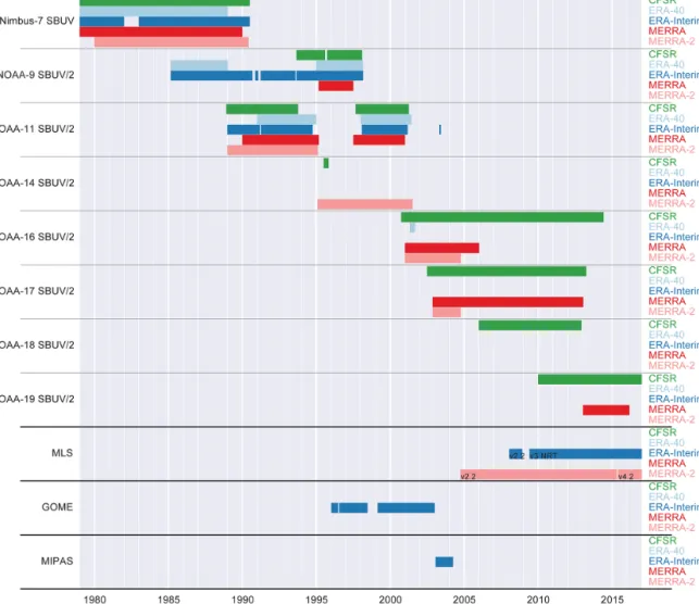
In this section, we compare SBUV TCO data to reanalysis products over the 1981–2010 climatology period. Figure 3 shows the seasonal cycle in total column ozone from SBUV as a function of latitude and month. Also shown are the differences between TOMS/OMI and SBUV, and between the different reanalyses and SBUV. The climatological TCO fields of the TOMS/OMI and the reanalyses are given as line contours in the difference plots. Figure S1 in the Supple- ment shows the equivalent comparison for TOMS/OMI data.

The reanalyses all reproduce the major features of the seasonal cycle and latitudinal distribution of TCO. This agreement is not surprising given that all of the reanalyses shown in Fig. 3 assimilate TCO data from one of the two satellites (Fig. 1). As such, the comparisons here do not represent independent validation of ozone in reanalyses, but rather represent a test of the internal consistency of the ozone data assimilation system. Hence it is not surprising that MERRA and MERRA-2 generally perform better against SBUV than against TOMS/OMI while ERA-Interim and JRA-55 generally perform better against TOMS/OMI than against SBUV, since MERRA and MERRA-2 assimilate SBUV (but not TOMS/OMI), while ERA-Interim and JRA-55 primarily assimilate TOMS/OMI (but not SBUV).

Although the reanalysis TCO fields look quite similar, a handful of widespread biases are revealed by considering the differences between reanalyses and observations. The agreement between the two observational TCO data sets is within approximately±6 DU (2∼3 %), with SBUV generally hav- ing smaller values in the tropics and larger values at high latitudes relative to TOMS/OMI. Differences between the reanalyses and the TCO observations are generally slightly larger than the difference between the two observational data sets. ERA-40 produces substantially larger TCO values than observed, particularly at higher latitudes. JRA-25 contains

(12)

Figure 3.Zonal and monthly mean total column ozone climatology over 1981–2010 from SBUV observations(a), along with the absolute differences between each reanalysis and SBUV. The difference between TOMS/OMI and SBUV is also shown(b).(c–i)Line contours show each reanalysis’ respective climatology, and the shading shows differences from SBUV, with cool (blue) colors representing negative values and warm (red) colors representing positive values. Both climatology and observational references to calculate differences for ERA-40 are for the time period January 1981–August 2002 in order to avoid sampling issues.

significantly smaller TCO values than observed (∼10 DU less), except during the springtime at high southern latitudes.

For reanalyses that only (or mainly) assimilate UV- based retrievals, the winter hemisphere high latitudes remain largely unconstrained by data assimilation. The impact of the TCO observations may also be limited by filtering choices.

For example, assimilated observations are filtered to exclude low solar elevation angles (less than 10^◦for TOMS and less than 6^◦for SBUV) in both ERA-40 and ERA-Interim. This filtering further limits observational impacts on the ozone analyses at higher latitudes. Hence, for ERA-Interim, before the start of the Aura MLS assimilation in 2008, high-latitude ozone fields essentially reflect the effects of transport and the ozone parameterization used. For ERA-40, Dethof and Hólm (2004) showed that the ozone model produces high biases in ozone concentrations at high latitudes ranging from

∼20 DU in the summer hemisphere to∼50 DU in the winter hemisphere, which is broadly consistent with the comparison shown in Fig. 3.

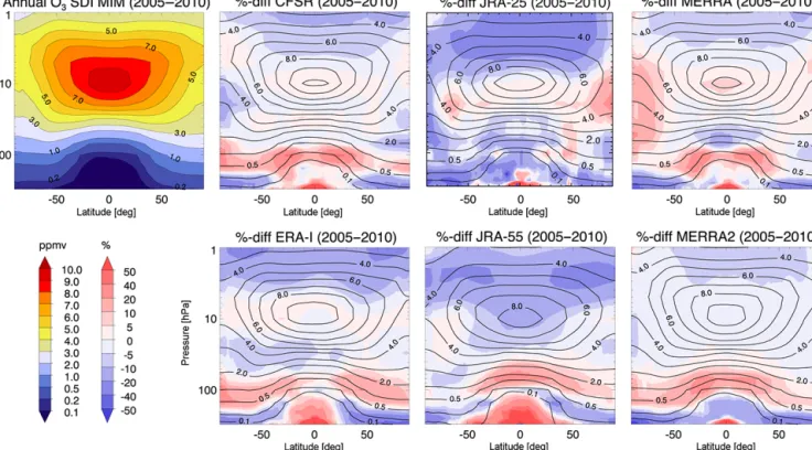
4.2 Zonal mean ozone cross sections

In this section, we compare zonal mean multi-annual mean cross sections of ozone between the different reanalyses and the SDI MIM. We perform the comparison for 2005–2010

using the subset of instruments described in Sect. 3.3. This shorter period has been chosen to avoid sampling issues that could be introduced by changes in instrument availability, which could alter sampling patterns, or trends in the constituents, such as the increase in ozone depletion from the 1970s to the mid-1990s. ERA-40 is excluded from this and all other comparisons with the SDI MIM because it ended in 2002.

Figure 4 shows multi-annual zonal mean ozone from the SDI MIM and the relative differences between each reanalysis and the SDI MIM (calculated as 100·(R_i−MIM)/MIM, whereR_i is the reanalysis field). Also indicated using contours are the climatological ozone distributions of the reanalyses. The reanalyses all capture the general zonal mean distribution of ozone, including the global maximum in the ozone volume mixing ratio in the tropical middle stratosphere and the tropopause-following isopleths immediately above the tropopause. Among the reanalyses, MERRA-2 best reproduces this overall structure, with relative differences within±5 % throughout the middle and upper stratosphere.

MERRA, CFSR, and ERA-Interim also perform generally well, but with MERRA overestimating concentrations in the ozone maximum (∼10 hPa) relative to the SDI MIM. ERA- Interim shows relatively good agreement in the middle stratosphere, with biases smaller than±5 %, but includes a low

(13)

Figure 4.Multi-annual zonal mean ozone cross sections averaged over 2005–2010 for the SPARC Data Initiative multi-instrument mean (SDI MIM) (upper left), along with the relative differences between reanalyses and observations as(R_i−MIM)/MIM·100, whereR_iis a reanalysis field (shading, other panels). Also shown in line contours are the respective zonal mean climatologies for the different reanalyses.

bias with magnitudes greater than 10 % in the upper stratosphere. All reanalyses show biases exceeding±10 % in the lowermost stratosphere, at pressures greater than 100 hPa.

JRA-55 is an improvement relative to JRA-25, particularly in the polar regions. Negative biases in JRA-55 have approximately halved in the middle and upper stratosphere compared to JRA-25. However, JRA-55 also shows somewhat higher positive biases around the tropical upper troposphere and lower stratosphere than JRA-25. It is worth noting that the diurnal cycle in ozone has not been explicitly accounted for in the observational MIM. Neglecting the diurnal cycle potentially contributes to differences between the reanalyses and observations in the upper stratosphere and lower mesosphere.

All reanalyses except the JRA products produce a positive bias in ozone in the Southern Hemisphere (SH) lower stratosphere. This indicates an inability to simulate Antarc- tic ozone depletion accurately due to a combined effect of limited data coverage, data filtering, and limitations of the reanalyses’ chemistry schemes at high latitudes (Sect. 4.1).

A dipole is apparent in the CSFR and ERA-Interim biases, with a high bias near ∼100 hPa located below a low bias near∼10 hPa. This dipole may reflect a lack of information about the vertical location of the ozone hole in the TCO and SBUV observations assimilated by these systems. In contrast, MERRA includes a significant high bias (>10 %) at

southern high latitudes that extends throughout the stratosphere.

4.3 Ozone monthly mean vertical profiles and seasonal cycles

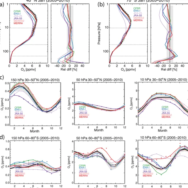
Figure 5a and b show vertical profiles of ozone for January (2005–2010 average) for the reanalyses and the SDI MIM at two different latitudes, 40^◦N and 70^◦S, respectively, along with the relative differences for each reanalysis with respect to the MIM. In addition, Fig. 5c and d show the seasonal cycles of ozone for three different pressure levels at 40^◦N and 70^◦S, respectively. The vertical profiles and the seasonal cycles reveal seasonal information on reanalyses–observation differences that expands upon the annual zonal mean evaluation presented in Sect. 4.2. In general, the results shown reinforce the conclusions of the previous section.

Most reanalyses resolve the vertical distribution in January reasonably well at both latitudes, in particular in the middle stratosphere between around 50 and 5 hPa. MERRA-2, MERRA, and CFSR perform particularly well. JRA-25, on the other hand, is a clear outlier that produces too little ozone in the vicinity of the maximum. JRA-55 and ERA-Interim also underestimate ozone concentrations in the upper stratosphere by between 10 and 20 %, but are not as strongly biased as JRA-25 (which produces differences of more than 30 %).

All reanalyses show larger percentage differences from the

(14)

Figure 5.Multi-annual mean vertical ozone profiles over 2005–2010 for January at(a)40^◦N and(b)70^◦S from the SPARC Data Initiative multi-instrument mean (SDI MIM) (black) and the six reanalyses (colored). Absolute values are shown in the left panels and relative differences in the right panels for each comparison. Relative differences are calculated as(R_i−MIM)/MIM·100, whereR_iis a reanalysis profile.

Black dashed lines provide the±1σuncertainty (as calculated by the SD over all instruments and years available) in the observational mean.

Horizontal dashed lines in grey indicate the pressure levels (150, 50, and 10 hPa) for which seasonal cycles are shown in panels(c, d)for the two latitude ranges 30–50^◦N and 60–80^◦S, respectively. In the lower panels, the SDI MIM uncertainty is shown using grey shading.

MIM in the lower part of the profile at pressures greater than 100 hPa. The reanalyses seem to overestimate ozone at around 150 hPa by 20 % in the southern high latitudes, pos- sibly related to not capturing accurately enough the extent of ozone depletion during spring. Below 200 hPa at both latitudes, all reanalyses underestimate observed ozone values.

The agreement between the reanalyses and observations varies by month, as can be seen in Fig. 5c and d, which show the annual cycle for selected pressure levels (150, 50, and 10 hPa) and somewhat extended latitude bands of 30–50^◦N and 60–80^◦S, respectively. The agreement in the ozone sea-

sonal cycle between the SDI observations and the reanalyses is better at the Northern Hemisphere (NH) mid-latitudes (where the seasonal cycles have a simple sinusoidal structure) than at the SH high latitudes. In the NH at 50 and 150 hPa, ozone reaches its annual maximum during boreal spring and its annual minimum during autumn, attributable to the strong seasonality in the Brewer–Dobson circulation.

The seasonal cycle is shifted at 10 hPa, with a maximum in summer and a minimum in winter, attributable mostly to ozone photochemistry. Most of the reanalyses produce a fairly accurate ozone evolution at these levels, with ex-

(15)

ceptions as follows: at 150 hPa, JRA-55 shows a strong low bias when compared to both observations and the other reanalyses during the NH winter/spring months. All the other reanalyses tend to overestimate the absolute ozone values, but agree rather well with the seasonal cycle in the observations in terms of amplitude and phase. At 50 hPa, the seasonal cycle produced by JRA-55 shows a more gradual de- cline in ozone concentrations into autumn relative to both observations and other reanalyses. ERA-Interim, MERRA, and CFSR at 10 hPa tend to overestimate ozone during spring and early summer, while JRA-55 (JRA-25) tends to underestimate (overestimate) ozone during fall and winter.

Seasonal cycles at SH high latitudes have a more complex structure than those at the NH mid-latitudes due to generally weaker downwelling in the Brewer–Dobson circulation and the influence of Antarctic ozone depletion. As a conse- quence, the reanalyses have more difficulty in capturing the seasonal cycle. At 10 hPa, MERRA-2 shows the best agreement with the observations. CFSR also follows the observations relatively well but overestimates the amplitude of the seasonal cycle, primarily because of values that are too low during May through July. MERRA and JRA-25 are outliers in that they do not contain the strong annual minimum observed during late austral autumn and early winter. At 50 hPa, MERRA and JRA-25 agree better with observations than at 10 hPa, but still underestimate austral springtime ozone depletion. Finally, at 150 hPa, the seasonality in the reanalyses varies widely and is inconsistent with that in the observations, with the exception of MERRA, which produces the most realistic seasonal cycle amplitude. MERRA-2 shows the closest agreement with observations at all levels except for 150 hPa, which is the next to lowest valid level of the MLS v2.2 ozone retrievals that it assimilates.

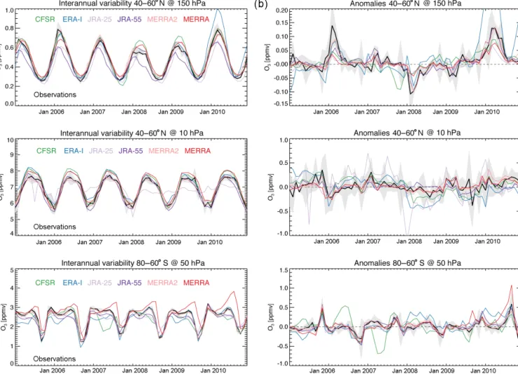
4.4 Ozone interannual variability

Figure 6 shows time series of interannual variability of ozone and its anomalies in the SDI MIM and reanalyses during 2005–2010. The anomalies, which are calculated for each reanalysis by subtracting multi-year monthly means averaged over 2005–2010 from the monthly mean time series, are a good indicator of how well physical processes (such as transport) are represented in reanalyses. Time series are shown for the SH high latitudes (averaged over 60–80^◦S) at 50 hPa, and for the NH mid-latitudes (40–60^◦N) at 150 and 10 hPa.

In all cases, MERRA-2 produces the closest match with the SDI MIM in terms of both the absolute values and the structure of its interannual variability. This agreement highlights the benefit of assimilating vertical profile observations from a limb-viewing satellite instrument, although it has to be noted that the comparison is not done against truly independent observations in this case, since Aura MLS is included in the SDI MIM. MERRA-2 is an evident improvement over MERRA, which tends to disagree with the absolute ozone values of the observations at 150 hPa and to overestimate them at 10 hPa,

and to underestimate interannual variability at both levels at the NH mid-latitudes. JRA-55 also shows clear improvement relative to JRA-25 with respect to the amplitude and structure of interannual variability, at least at 10 hPa at the NH mid- latitudes. Large excursions seen in JRA-25, such as the sudden drop in ozone at the beginning of 2008, are not present in JRA-55 or in the observations.

Although ERA-Interim ozone mean values mostly agree well with observations, the amplitude of its interannual variability is larger than observed. In particular, ERA-Interim overestimates the negative anomaly at NH mid-latitudes at 10 hPa and the positive anomaly at SH high latitudes at 50 hPa during 2008. The largest differences appear to affect ERA-Interim from mid-2009 when the assimilation of Aura MLS data restarted with the (v3) NRT product after months of data unavailability. CSFR also produces large interannual excursions during certain years (e.g., during spring 2006 and 2007 at 50 hPa in SH high latitudes). This issue may be related to SBUV only offering measurements between Septem- ber to March, so that the assimilation system is not well constrained during the remainder of the year.

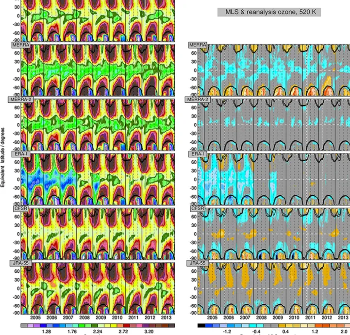
4.5 Ozone time series in equivalent latitude coordinates Equivalent latitude (EqL) is a common vortex-centered coordinate used in studies of the stratosphere (e.g., Butchart and Remsberg, 1986; Manney et al., 1999, and references therein). This coordinate is also useful as a geophysically based coordinate in the UTLS (e.g., Santee et al., 2011), although interpretation becomes more complicated in this context (e.g., Manney et al., 2011; Pan et al., 2012). The equivalent latitude of a potential vorticity (PV) contour is defined as the latitude of a circle centered about the pole enclos- ing the same area as the PV contour (see Hegglin et al., 2006, for a visual illustration). Figure 7 shows the time series of v4 MLS ozone (Sect. 3.4) for late 2004 through 2013 in the lower stratosphere (520 K), along with differences between MERRA, MERRA-2, ERA-Interim, CFSR, and JRA-55 and MLS ozone at the same level. MLS ozone is interpolated to isentropic surfaces using temperatures from MERRA. The EqL ozone time series are then produced using a weighted average of MLS data in EqL and time, with data also weighted by measurement precision (e.g., Manney et al., 2007, 1999). Figures S2 and S3 show the equivalent evaluation for the 350 and 850 K potential temperature levels.

Figure 7 reveals that MERRA-2 matches MLS more closely over the full period than do the other reanalyses.

This is expected because the stratospheric ozone reanalyses in MERRA-2 are largely constrained by the MLS stratospheric ozone profiles (v2 for the period shown here). This agreement is especially apparent during Antarctic winter and spring, when other assimilated ozone products (e.g., SBUV/2 and TOMS) cannot provide measurements due to darkness and simplified chemical parameterizations cannot adequately

(16)

Figure 6.Interannual variability(a)and deseasonalized anomalies(b)for ozone during 2005–2010 for the SPARC Data Initiative multi- instrument mean (SDI MIM, black) and the six reanalyses (colored). Results are shown for three different pressure levels and latitude ranges (top to bottom: 50 hPa at 60–80^◦S, 10 hPa at 20^◦S–20^◦N, and 100 hPa at 40–60^◦N). Grey shading indicates observational uncertainty (±1σ) calculated as the SD over all instruments and years available.

represent heterogeneous loss processes. The improved vertical resolution of MLS relative to SBUV/2 also better con- strains the structure of the ozone hole, which is vertically limited. ERA-Interim also shows close agreement with MLS during the periods when it assimilates MLS ozone products (2008 and mid-2009 through present). The change in behav- ior in ERA-Interim between these time periods and the general similarity of PV contours among the different reanalyses suggest that the poor representation of ozone in these regions is due more to the lack of assimilated ozone data than to the representation of polar dynamical processes in reanalyses.

Biases in the reanalyses that do not assimilate MLS and OMI ozone vary in magnitude and sign, not only among the reanalyses, but also with altitude and latitude (see also Figs. S2–S3). High biases in MERRA and CFSR ozone during Arctic winter may be partially related to inadequate representations of ozone chemistry and an overall lack of measurements. We speculate that the latter is dominant due to the appearance of these biases even during years with min-

imal observed chemical ozone loss. JRA-55 biases increase strongly with altitude (cf. Figs. S2 and S3), becoming even larger in the upper stratosphere. These large biases suggest that column ozone alone is insufficient to properly constrain the vertical distribution of the ozone analyses, but that assimilation of vertically resolved observations during polar night can provide a much better constraint on ozone in these regions.

4.6 Ozone quasi-biennial oscillation signals

Variations in transport and chemistry associated with the quasi-biennial oscillation (QBO) in tropical zonal wind are among the largest influences on interannual variability in equatorial ozone. The QBO signal in tropical ozone has a double-peaked structure with maxima in the lower (50–20 hPa) and middle-to-upper (10–2 hPa) stratosphere (Hasebe, 1994; Zawodny and Mccormick, 1991). Ozone is mainly under dynamical control below 15 hPa, where the

(17)

Figure 7.Comparison of the equivalent latitude–time evolution of each reanalysis ozone field and MLS on the 520 K isentropic surface (∼50 hPa;∼20 km altitude) during Aura mission September 2004–December 2013.(a)Mixing ratios (ppmv) for MLS and the reanalyses MERRA, MERRA-2, ERA-Interim, CFSR, and JRA-55 (top to bottom).(b)Differences (ppmv) between each reanalysis and MLS (R_i− MLS). Overlays are scaled potential vorticity (Manney et al., 1994) contours of 1.4 and 1.6×10⁻⁴s⁻¹from the corresponding reanalysis, which are intended to represent the wintertime polar vortex edge. Dynamical fields for the MLS panel are from MERRA.

QBO signal results primarily from changes in ozone transport due to the QBO-induced residual circulation. In contrast, ozone is under photochemical control above 15 hPa.

The QBO signal in these upper levels is understood to arise from a combination of QBO-induced temperature variations (Ling and London, 1986; Zawodny and Mccormick, 1991) and QBO-induced variability in the transport of NO_y(Chip- perfield et al., 1994). A realistic characterization of the time–

altitude QBO structure is an important aspect of physical consistency in ozone data sets.

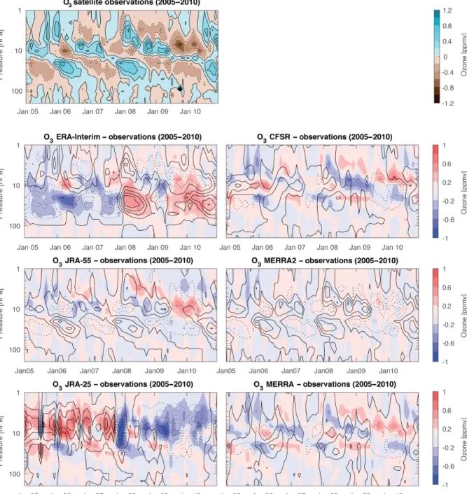
Figure 8 shows time–altitude cross sections of deseasonalized ozone anomalies from 2005 to 2010 from the SDI MIM, along with the differences between the ozone anomaly fields from the reanalyses and the SDI MIM. The climatological QBO anomaly fields of the reanalyses are given as contours in the difference plots. Combined ozone mea-

(18)

Figure 8.QBO ozone signal from the SPARC Data Initiative observations (upper left) during 2005–2010, defined as altitude–time cross sections of deseasonalized ozone anomalies averaged over the 10^◦S–10^◦N tropical band. Observations are based on three satellite data sets.

The other panels show the differences in QBO ozone signals between each reanalysis and the observations (R_i−MIM, shaded contours), with the black line contours showing the QBO ozone signal generated by each corresponding reanalysis.

surements from the limb-viewing satellite instruments show a downward propagating QBO ozone signal with a shift in the phase around 15 hPa. All reanalyses exhibit some degree of quasi-biennial variability; however, differences are evident in the phase, amplitude, vertical extent, and downward propagation of these signals. The largest deviations from observations are in JRA-25, which displays positive anomalies from 2005 to mid-2007 followed by negative anomalies from mid-2007 through 2010 in place of the QBO sig-

nal above 15 hPa. In contrast, ERA-Interim shows predomi- nantly negative anomalies in the 100–10 hPa pressure range before 2008 and positive anomalies afterwards. The changes in ERA-Interim coincide with the beginning of the assimilation of Aura MLS profiles beginning in 2008, which caused a shift to positive anomalies. Negative anomalies are present during the first half of 2009, when no MLS data were assimilated, followed by positive anomalies after the reintroduction of MLS data in June 2009 (Sect. 2.5).