Water Vapor Calibration: Using a Raman Lidar and Radiosoundings to Obtain Highly Resolved Water Vapor Profiles

Article

Water Vapor Calibration: Using a Raman Lidar and Radiosoundings to Obtain Highly Resolved Water Vapor Profiles

Birte Solveig Kulla ^1,2, * and Christoph Ritter ^1, *

1

Alfred-Wegener-Institut, Telegrafenberg A45, 14473 Potsdam, Germany

2

Institut für Geophysik und Meteorologie, Universität zu Köln, Pohligstr. 3, 50969 Cologne, Germany

* Correspondence: birte.kulla@awi.de (B.S.K.); christoph.ritter@awi.de (C.R.)

Received: 28 January 2019; Accepted: 5 March 2019; Published: 13 March 2019

Abstract: We revised the calibration of a water vapor Raman lidar by co-located radiosoundings for a site in the high European Arctic. For this purpose, we defined robust criteria for a valid calibration. One of these criteria is the logarithm of the water vapor mixing ratio between the sonde and the lidar. With an error analysis, we showed that for our site correlations smaller than 0.95 could be explained neither by noise in the lidar nor by wrong assumptions concerning the aerosol or Rayleigh extinction. However, highly variable correlation coefficients between sonde and consecutive lidar profiles were found, suggesting that small scale variability of the humidity was our largest source of error. Therefore, not all co-located radiosoundings are useful for lidar calibration. As we assumed these changes to be non-systematic, averaging over several independent measurements increased the calibration’s quality. The calibration of the water vapor measurements from the lidar for individual profiles varied by less than ± 5%. The seasonal median, used for calibration in this study, was stable and reliable (confidence ± 1% for the season with most calibration profiles). Thus, the water vapor mixing ratio profiles from the Koldewey Aerosol Raman Lidar (KARL) are very accurate. They show high temporal variability up to 4 km altitude and, therefore, provide additional, independent information to the radiosonde.

Keywords: lidar; Raman shift; AWIPEV; Svalbard; water vapor; water vapor calibration; radiosonde;

GRUAN; Vaisala; atmosphere

1. Introduction

In the Arctic, average temperatures rise twice as fast as on global average; the so-called “Arctic Amplification” of global warming. This regional pattern of global warming with its pronounced warming north of the Arctic Circle is associated with various feedbacks and still subject of ongoing research [1]. One of the hot spots of warming is the eastern European Arctic between Spitsbergen and the Kara Sea. In Ny-Ålesund at the west coast of Spitsbergen (79.9 ^◦ N and 11.9 ^◦ E), where the measurements for this study took place, a warming of 3 K per decade in winter (DJF) was observed over the past 26 years [2]. Roughly a quarter of this warming can be attributed to an increased advection of warm and moist air from the North Atlantic into the European Arctic [3].

Water vapor is the strongest and most variable greenhouse gas [4] and its vertical distribution determines its radiative impact [5]. A clear impact (at least of stratospheric) water vapor on the climate of the last decades has been proven [6]. Assessing the role of tropospheric water vapor, however, is very challenging as feedbacks with clouds and aerosol must be considered and are not fully understood yet. A systematic deviation between aerosol extinction from remote sensing and in-situ measurements in the Arctic boundary layer [7] indicates that hygroscopic growth of aerosol needs to be investigated

Remote Sens. 2019, 11, 616; doi:10.3390/rs11060616 www.mdpi.com/journal/remotesensing

over the full atmospheric column. Hence, monitoring water vapor, especially in the Arctic atmosphere, is an important task. Addressing the integrated water vapor under the usually very dry conditions of the Arctic atmosphere in winter is not easy and subject of ongoing research [8].

There are two major approaches to measure water vapor with lidar systems: either using the differential absorption technique (e.g., [9]) or, as was done in this study, using the Raman scattering effect (e.g., [10–12]). Calculating the ratio between the inelastically scattered lidar profile of water vapor and nitrogen, with a minor correction for wavelength-dependent extinction, gives a signal proportional to the water vapor mixing ratio (e.g., [13]). To derive the humidity from the lidar signal, a calibration is necessary to link the ratio of the lidar profiles to the actual water vapor mixing ratio.

This calibration can be done by either measuring the transmission of the different detection branches of the lidar or comparison of the lidar product with external instruments. For the first method, determination of the transmission of both branches (nitrogen and water vapor) of the lidar system [14] has been proposed. For this transmission measurement, skylight or a precise lamp [15]

may be used. While this method is completely independent of other instruments, it introduces more components to the lidar and more effort during data acquisition. The second method uses humidity profiles from external instrumentation such as radiosondes (e.g., [16,17]), microwave (e.g., [18,19] or photometer data (e.g., [20] for calibration. In addition, a hybrid technique, employing both a tungsten lamp and radiosonde, has also been introduced [21].

While principally a suite of many different instruments measure the water vapor at the supersite of Ny-Ålesund [22], not all of them are appropriate for lidar calibration. GPS measurements are handicapped by the large footprint of satellites in comparison to KARL at our coastal site with challenging orography posing problems [23].

A HATPRO microwave radiometer only covered a short period of parallel measurements to the lidar. In addition, radiometer humidity profiles have high uncertainties [24] and the integrated water vapor, which is considered to be more reliable, cannot be used for calibration because KARL lacks exact measurement in the lowermost 350 m. Thus, with the incomplete overlap of the telescope, a reliable integrated signal cannot be derived.

In addition, (star-)photometer measurements of water vapor in the polar night have not been analyzed in detail yet and can therefore not be used for lidar calibration. Thus, we chose radiosounding measurements for lidar calibration in this work as they provide continuous height-resolved data at high accuracy. Its in-situ measurements have the huge advantage of high vertical resolution, which can then be resampled to the chosen resolution of our lidar. Disadvantages and uncertainties of radiosoundings are essentially eliminated by carefully choosing calibration constraints, which are explained in this work. For Ny-Ålesund, a calibration technique has been established with data from the dark seasons 2015/2016 and 2016/2017. Only few and short measurements with simultaneous radiosounding measurements were available then. However, in 2018, parallel to the Year Of Polar Prediction (YOPP) campaign with a higher frequency of radiosoundings, longer lidar measurements were carried out.

Thus, in winter 2018, 451 hours of lidar measurement were acquired with 21 simultaneous profiles of radiosoundings, which were according to our specifications suited for lidar calibration.

Hence, the aim of this work was to revise the water vapor calibration of a lidar by radiosondes for the Arctic site of Ny-Ålesund. The precision with which a lidar calibration can be performed was determined for our system. After a quick overview of the already established theory, we explain our calibration constraints, compare the GRUAN to the Vaisala humidity and present an error analysis for the mixing ratio profile in the lidar. By using a correlation coefficient between the mixing ratio profiles of radiosonde and lidar, it is shown that correlations below 0.95 could not be explained by noise in the data but indicate different meteorological conditions even for contemporaneous profiles.

2. Theory and Background

The Koldewey Aerosol Raman lidar (KARL) is a multi-wavelength Raman lidar for tropospheric

and stratospheric research. Among others, the system is part of the Network for the Detection of

Atmospheric Composition Change (NDACC, see: http://www.ndsc.ncep.noaa.gov/), to which it contributes with aerosol properties. The laser emits laser pulses at 1064 nm (IR), 532 nm (VIS) and 355 nm (UV) at 50 Hz with approximately 10 W per wavelength. Raman shifted lines are detected at 407 nm and 660 nm as well as at 387 nm and 607 nm, for the Stokes lines from H 2 O and N 2 molecules, respectively. The field-of-view of the 70 cm collecting telescope is about 1 mrad (for more details to the setup, see [25]). With the dry atmospheric conditions during polar night, only the counting signal is used and channel combination problems, as discussed in [26], do not have to be taken into account. As the UV signal is less noise-prone, the focus of this work lies on the signal from the 407 nm and 387 nm channels. The transmission-corrected signals from those two channels are proportional to the water vapor and nitrogen density (ρH ₂ O and ρN ₂ ) in the respective height bin. As nitrogen is homogeneously distributed in the atmosphere, it is also proportional to the density of dry air. Therefore, the ratio between the two densities is proportional to the volume mixing ratio of water vapor (VMR) [27], which is then also proportional to the mass mixing ratio (MMR).

V MR = ^{ρ H}

^O

ρ _air = ^{ρ H}

^O

K _N

→air ρ _N

= C T ₄₀₇ ^Ray · T ₄₀₇ ^aer · P 407

T ₃₈₇ ^Ray · T ₃₈₇ ^aer · P 387

≡ C · S _lidar (1)

Here, C is the lidar calibration constant that needs to be fixed by comparison with additional measurements and S _lidar is the uncalibrated water vapor signal from the lidar. The expressions T ₃₈₇ ^xx and T ₄₀₇ ^xx denote the transmission of the backscattered light through the atmosphere due to Rayleigh and aerosol extinction at the two wavelengths (λ). The aerosol transmission depends on the volumetric aerosol extinction coefficient α ^aer _λ by:

T _λ = exp − Z _z

z

α ^aer _λ d ˆ z

> exp (− AOD _λ ) (2)

As lidar systems usually do not sound the entire atmosphere but only a limited vertical range, from z ₀ to z in Equation (2), the integral of the aerosol extinction is always smaller than the aerosol optical depth (AOD) measured by photometers.

Frequently, the aerosol extinction follows a power-law of wavelength with the so-called Ångström exponent A with A < 0. Hence, the ratio of the aerosol transmission terms at the two wavelengths can be expressed by:

T ₄₀₇ ^aer ( z )

T ₃₈₇ ^aer ( z ) = exp ^Z z

z

α ^aer ₃₈₇ · 1 − ( ⁴⁰⁷

387 ) ^A d ˆ z

(3) Thus, the error in the water vapor retrieval due to aerosol rises with the aerosol load (α ^aer ₃₈₇ ) and its spectral slope (A). A large extinction caused by small particles has the higher impact, whereas sub-visible clouds (small extinction, A ≈ 0) are not critical. In our work, we set A = − 1.2, which is close to the long-term average for Ny-Ålesund in March [28].

Given the low water vapor content in the atmosphere above Ny-Ålesund, the signal is very weak and measurements are limited to the dark period. For this study, we found measurements with a sun elevation below − 10 ^◦ suitable. To assess data quality, the signal-to-noise ratio (SNR) was calculated. Therefore, we expressed the lidar signal P in the units of photons, which are clearly identified as individual “steps” in the counting signal. Let the constant c be the conversion between one photon and the measured lidar signal P in arbitrary units. Then, c · P is the lidar signal in the unit photons. (For Licel transient recorders, c might be the inverse of laser shots written in one data file.) In these units, the error of the lidar signal due to photon noise can be expressed by the standard deviation, which is the square root of the signal c · P. Moreover, we considered an electronic, or photon-independent error source, which here is called E [29]. Apart from all photon-independent noise sources, E considers effects of a wrong background subtraction as well. The SNR then is defined as

SNR = √ ^cP

cP + cE (4)

Data for this work were processed with 60 m / 10 min resolution without any further filtering during the evaluation.

3. Calibration

As the water vapor signal (P407) is weaker than the nitrogen signal (P987) by much more than one order of magnitude, only the quality of the water vapor signal (P407) was assessed for further analysis.

The main source of noise is sunlight. Here, for the resolution of 60 m and 10 min, we mostly found data with sun altitudes below − 10 ^◦ suitable. Depending on the signal strength, the signal-to-noise ratio SNR typically dropped below 10 at an altitude between 3000 and 4000 m. At the expense of resolution, higher altitudes can be reached and profiles during twilight might fulfill the criteria for calibration. However, due to the observed high variability of the humidity, this is only recommendable to some extent.

In addition to this noise in the lidar signal, possible error sources for the calibration are: incorrect measurements by the radiosonde, inaccuracies when converting relative humidity (rh) to the water vapor mixing ratio, and differences in probed air masses, either due to the drift of the radiosonde or due to temporal differences. To minimize the effects these errors might have on the calibration, five criteria were established. Table 1 gives an overview on the requirements made to the data for them to be considered suitable for calibration.

Table 1. Requirements for data to be elected for calibration.

Requirement Restriction

no/little noise SNR of P407 > 10

not within the incomplete lidar overlap altitude >400 m

not within a range of known radiosounding bias not within a cloud (rh < 0.9) and no dry bias (T > − 40

C) not too much time difference using the measurement closest to radiosounding start time,

max. 1 h time difference

both measurements have probed similar air masses Pearson Correlation Coefficient of log > 0.95 (min. 20 pairs per profile have to fulfill the criteria)

Known biases in radio sounding measurements [30] were excluded by using measurements with temperatures above − 40 ^◦ C and relative humidity below dew point. Moreover, only very reliable lidar measurements at heights with a complete overlap and SNR above 10 are taken into account. We show in Section 6 that this condition guarantees for our data that the remaining noise in the lidar signal does not degrade the retrieval of the calibration constant further.

Furthermore, a Pearson correlation between the logarithm of the two mixing ratio profiles (radio sounding and lidar) was calculated to assure that the same or at least very similar air masses were probed. This is relevant to correct for the sonde’s drift and possible small-scale fluctuations of the humidity. The correlation between the signal ratio (S _lidar ) and the water vapor mixing ratio from the radiosonde (w) is known to be linear [31], thus the correlation between S _lidar and w should be unity if noise is not an issue and both measurements have indeed probed the same air masses. As very low values have an equally high impact on the calibration as high values, logarithmic profiles are compared. If the correlation was higher than 0.95, the profiles were considered to match and the air masses had hardly changed between the two measurements. The limit of r > 0.95 is justified in Section 6 by an error estimation.

A example of a consistent mixing ratio profile between lidar and radiosonde is depicted in Figure 1.

The heights in which the different rules would be applied are indicated. A valid determination of the

mixing ratio is possible for SNR lower than 10. The above-mentioned criteria to exclude data points

for calibration are meant to be strict. Only if all of them were given, the corresponding data point was

used to determine the lidar calibration constant.

T<-40°C

SNR < 10

rh > 0.9 altitude < 400, incompl. overlap

Figure 1. Exemplary lidar profile used for calibration (20 February 2018). Bins used for calibration (z

) are highlighted with green points. Conditions under which heights are excluded from calibration as in Table 1 due to deficiencies in lidar (green) or radiosonde data (blue) are marked.

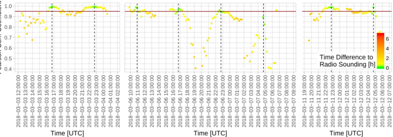
Figure 2 shows this Pearson correlation coefficient between the logarithms of w RS and S lidar . During a period of consistently clear sky in March 2018, lidar observations were compared to the radiosonde closest in time. Correlations very close to unity occurred when measurements were very close in time and air masses were relatively constant (see Figure 7 for comparison). With increasing temporal difference between the measurements, the correlation decreased, sometimes very rapidly.

The profiles closest to the start time of the radiosonde were considered to be the best fit. There were also occasions where co-located lidar and radiosonde measurements did not show a good agreement in the mixing ratio profile. In this case, profiles were excluded from the calibration. We come back to this fact in Section 6 and show that small scale fluctuations of the humidity profile are the most probable reason for this, as neither noise in the lidar nor the treatment of aerosol or the Rayleigh atmosphere could explain this variance.

It can be also seen in Figure 2 that sometimes the correlation oscillated around 0.95 for our data.

For this reason, we included the additional criterion of a maximum time difference of one hour between lidar and sonde for calibration to guarantee that the same air masses were probed.

●

●

●

●

●

●

●

●

●

●

●

●

●

●●

●

●

●

●

●●

●

●●●●●●

●●

●●●

●

●●

●

●

●

●●●●●●●●

●●●●●●●●●●●●●●●●

●

●

0.4 0.5 0.6 0.7 0.8 0.9 1.0

2018−03−03 12:00:00 2018−03−03 13:00:00 2018−03−03 14:00:00 2018−03−03 15:00:00 2018−03−03 16:00:00 2018−03−03 17:00:00 2018−03−03 18:00:00 2018−03−03 19:00:00 2018−03−03 20:00:00 2018−03−03 21:00:00 2018−03−03 22:00:00 2018−03−03 23:00:00 2018−03−04 00:00:00 2018−03−04 01:00:00 2018−03−04 02:00:00 Time [UTC]

Pearson Corr. Coefficient

●

●

●●●

●●

●●

●

●●

●●●●

●

●

●●

●●●●

●●

●●●●

●

●

●●●

●

●●

●

●

●

●

●

●

●●

●

●

●●●

●

●●●●●●●●●

●●●●●●●

●●●

●

●

●

●

●●

●●

●

●

●

●

●

●●●

●●

●

0.4 0.5 0.6 0.7 0.8 0.9 1.0

2018−03−06 10:00:00 2018−03−06 11:00:00 2018−03−06 12:00:00 2018−03−06 13:00:00 2018−03−06 14:00:00 2018−03−06 15:00:00 2018−03−06 16:00:00 2018−03−06 17:00:00 2018−03−06 18:00:00 2018−03−06 19:00:00 2018−03−06 20:00:00 2018−03−06 21:00:00 2018−03−06 22:00:00 2018−03−06 23:00:00 2018−03−07 00:00:00 2018−03−07 01:00:00 2018−03−07 02:00:00 2018−03−07 03:00:00 2018−03−07 04:00:00 2018−03−07 05:00:00 2018−03−07 06:00:00 2018−03−07 07:00:00 2018−03−07 08:00:00 2018−03−07 09:00:00 Time [UTC]

Pearson Corr. Coefficient

●

●●

●●●

●

●

●

●

●●●●●●●●●●●●

●

●●●●

●●●●●●●●●●●●●●●

●

●

●

●

●

●●

●

●

0.4 0.5 0.6 0.7 0.8 0.9 1.0

2018−03−11 19:00:00 2018−03−11 20:00:00 2018−03−11 21:00:00 2018−03−11 22:00:00 2018−03−11 23:00:00 2018−03−12 00:00:00 2018−03−12 01:00:00 2018−03−12 02:00:00 2018−03−12 03:00:00 2018−03−12 04:00:00 2018−03−12 05:00:00 2018−03−12 06:00:00 2018−03−12 07:00:00 Time [UTC]

Pearson Corr. Coefficient

0 2 4 6

Time Difference to Radio Sounding [h]

Figure 2. Pearson correlation coefficient between log ( w

) and log ( S

) at heights where data

would fulfill all other criteria to be selected for calibration (z

) during the nights from 3 March 2018 to

4 March 2018, 6 March 2018 to 7 March 2018 and 11 March 2018 to 12 March 2018. Colors indicate the

temporal difference between the start of the radiosonde and the lidar measurement. Red line shows

the threshold for minimal correlation applied here. Start of radiosounding measurement indicated by

black, dashed line.

For all remaining data-pairs ( w RS ( t _i , z _i ) , S _lidar ( t _i , z _i )) , a possible correction factor C _i was calculated.

w _RS ( t _i , z _i ) = S _lidar ( t _i , z _i ) C _i C i = ^{w RS}

S _lidar (5)

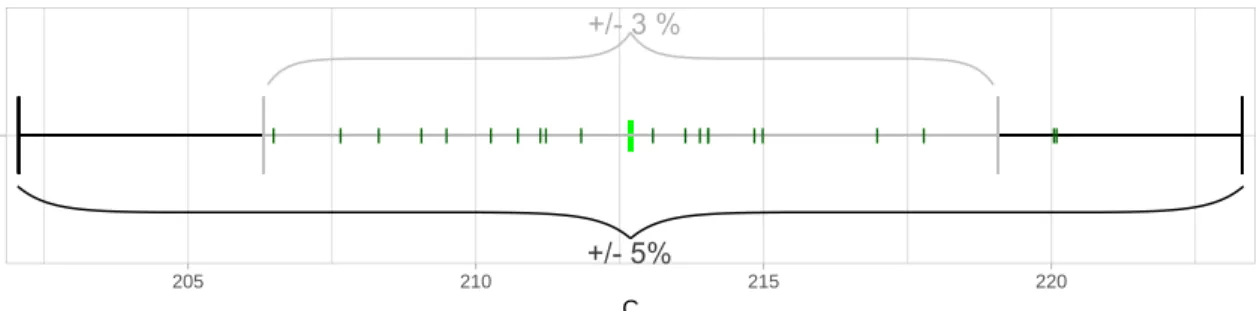
C i varies according to the deviations discussed above (see also Figure 4), and the median is relatively stable. Using the median of all those correction factors (C i ) that were needed at the particular heights z _i and fulfill the criteria specified in Table 1 can give one correction factor per profile t _i (dark green I in Figure 3).

IIIIIIIIIIIIIIIIIIIIIIIIIIIIIIIIIIIIIIIIIIIIIIIIIIIIIIIIIIIIIIIIIIIIIIIIIIIIIIIIIIIIIIIIIIIIIIIIIIIIIIIIIIIIIIIIIIIIIIIIIIIIIIIIIIIIIIIIIIIIIIIIIIIIIIIIIIIIIIIIIIIIIIIIIIIIIIIIIIIIIIIIIIIIIIIIIIIIIIIIIIIIIIIIIIIIIIIIIIIIIIIIIIIIIIIIIIIIIIIIIIIIIIIIIIIIIIIIIIIIIIIIIIIIIIIIIIIIIIIIIIIIIIIIIIIIIIIIIIIIIIIIIIIIIIIIIIIIIIIIIIIIIIIIIIIIIIIIIIIIIIIIIIIIIIIIIIIIIIIIIIIIIIIIIIIIIIIIIIIIIIIIIIIIIIIIIIIIIIIIIIIIIIIIIIIIIIIIIIIIIIIIIIIIIIIIIIIIIIIIIIIIIIIIIIIIIIIIIIIIIIIIIIIIIIIIIIIIIIIIIIIIIIIIIIIIIIIIIIIIIIIIIIIIIIIIIIIIIIIIIIIIIIIIIIIIIIIIIIIIIIIIIIIIIIIIIIIIIIIIIIIIIIIIIIIIIIIIIIIIIIIIIIIIIIIIIIIIIIIIIIIIIIIIIIIIIIIIIIIIIIIIIIIIIIIIIIIIIIIIIIIIIIIIIIIIIIIIIIIIIIIIIIIIIIIIIIIIIIIIIIIIIIIIIIIIIIIIIIIIIIIIIIIIIIIIIIIIIIIIIIIIIIIIIIIIIIIIIIIIIIIIIIIIIIIIIIIIIIIIIIIIIIIIIIIIIIIIIIIIIIIIIIIIIIIIIIIIIIIIIIIIIIIIIIIIIIIIIIIIIIIIIIII

I I I

I I I I I II I I III I I I II

C

205 210 215 220

C

+/- 3 %

+/- 5%

Figure 3. Calibration factor for winter 2017/2018. Light green I: median of all C

; dark green I: median of C

, when using only one profile at a time; grey: seasonal median of C

± 3%; black: seasonal median of C

± 5%.

This daily C varied within an order of ± 3% and was always below ± 5%. As we assumed the sources of error to be non-systematic, we could increase the quality of the calibration by increasing the sample size. We found no seasonal drift in these profile specific calibration factors (dark green), and, thus, it was valid to calculate the median over all correction factors at the specified heights in all suitable profiles ( C e _i , light green I in Figure 3) to determine one calibration factor per season.

We assumed that, due to consistent calibration criteria, all daily calibration constants were equal and that all errors were non-systematic (such as noise in the lidar data and drift of the sonde, which over a season may with equal frequency lead to a dry or wet bias in the sonde). If the lidar was at constant settings over time, the error of a seasonal calibration would then decrease by the square root of the number of individual calibrations. Hence, in our case, about 25 calibration profiles of a radiosonde were needed to reduce the insecurity of this seasonal calibration value to ± 1%.

4. Comparison of GRUAN and Vaisala Product

The radiosonde dataset from global Climate Observing System (GCOS) Reference Upper-Air Network (GRUAN) is considered a high quality radiosonde product. GRUAN data have the advantage of given uncertainties, and humidity measurements are more precise with an additional ground check at 100% relative humidity [30]. However, most of the correction happens at higher altitudes and under conditions that were excluded from the calibration. Thus, a comparison with a calibration using radiosounding measurements as derived by the Vaisala algorithm of RS92 showed very little deviation.

In the dark season 2017/2018, the RS41 was used at Ny-Ålesund. The GRUAN product for this type of sonde is not available yet.

Calibrating KARL measurements of the winter season 2016/2017 with both GRUAN-corrected

and Vaisala measurements gave a C e _i of 216 g/kg and 214 g/kg in our units, respectively. Thus, the

humidity measurements with the uncorrected data showed a slight dry bias. However, even with

the biased calibration result, the humidity measurement only deviated by less than 1%. In the year

before, a calibration with the Vaisala product yielded a drier result. Differences resulted mainly from

the fact that not all profiles were available at GRUAN standard. As we expect the RS41, which was