RV MARIA S. MERIAN Fahrtbericht / Cruise Report MSM63

(1)

GEOMAR REPORT

PERMO

Southampton – Southampton (U.K.) 29.04.-25.05.2017

Berichte aus dem GEOMAR

Helmholtz-Zentrum für Ozeanforschung Kiel

Nr. 37 (N. Ser.)

August 2017

RV MARIA S. MERIAN Fahrtbericht /

Cruise Report MSM63

(2)

(3)

PERMO

Southampton – Southampton (U.K.) 29.04.-25.05.2017

Berichte aus dem GEOMAR

Helmholtz-Zentrum für Ozeanforschung Kiel

Nr. 37 (N. Ser.)

August 2017

RV MARIA S. MERIAN Fahrtbericht /

Cruise Report MSM63

(4)

Herausgeber / Editors:

Christian Berndt and Judith Elger with contributions from cruise participants C. Böttner, R.Gehrmann, J. Karstens, S. Muff, B. Pitcairn, B. Schramm, A. Lichtschlag, A.-M. Völsch

GEOMAR Report

ISSN Nr.. 2193-8113, DOI 10.3289/GEOMAR_REP_NS_37_2017

Helmholtz-Zentrum für Ozeanforschung Kiel / Helmholtz Centre for Ocean Research Kiel GEOMAR

Dienstgebäude Westufer / West Shore Building Düsternbrooker Weg 20

D-24105 Kiel Germany

Helmholtz-Zentrum für Ozeanforschung Kiel / Helmholtz Centre for Ocean Research Kiel GEOMAR

Dienstgebäude Ostufer / East Shore Building Wischhofstr. 1-3

D-24148 Kiel Germany

Tel.: +49 431 600-0 Fax: +49 431 600-2805 www.geomar.de

(5)

Prof. Dr. Christian Berndt

GEOMAR Helmholtz Centre for Ocean Research Kiel Wischhofstr. 1-3, 24148 Kiel

Germany

Ph.: +49 431 6002273 Fax: +49 431 6002922 cberndt@geomar.de

MSM63 PERMO Cruise Report

Southampton – Southampton 29 April 2017 – 25 May 2017

Chief Scientist Leg 1: Prof. Dr. Christian Berndt Chief Scientist Leg 2: Dr. Judith Elger

Master: Björn Maaß

With contributions by Christoph Böttner, Romina Gehrmann, Jens Karstens, Sina Muff, Ben Pitcairn, Bettina Schramm, Anna Lichtschlag, Ann-Marie Völsch

May 2017

(6)

1 Cruise Summary ... 1

1.1 German ... 1

1.2 English ... 2

2 Paticipants ... 3

2.1 Principal Investigators ... 3

2.2 Scientific Party ... 3

3.3 Affiliations ... 4

3.4 Crew ... 5

3 Research Programm ... 6

3.1 Motivation ... 6

3.2 Aims of the Cruise ... 10

4 Narrative of the Cruise ... 11

5 Preliminary Results ... 15

5.1 Seismic Data Acquisition and Processing ... 15

5.2 OBS Experiments ... 20

5.3 Controlled Source Electromagnetic Surveys ... 23

5.4 Multibeam ... 33

5.5 Parasound ... 43

5.6. Chemistry and Hydrography ... 46

6 Ship’s Meterological Station ... 51

7 Station List MSM63 ... 51

8 Data and Sample Storage and Availability ... 51

9 Acknowledgements ... 52

10 References ... 52

Appendices ... 57

Appendix A: Station Book ... 57

Appendix B: OBS stations ... 125

Appendix C: Air gun shooting for OBS ... 126

Appendix D: Seismic profiles ... 128

(7)

Cruise report MSM63 1

1 Cruise Summary (C. Berndt)

1.1 German

Die hydraulische Permeabilität von Sedimentbecken variiert über mehrere Größenordnungen und auf verschiedenen Skalen. Da sie schwer zu messen und daher weitgehend unbekannt ist, ergeben sich daraus ernsthafte Probleme bei der numerischen Modellierung von Fluidzirkulation in Sedimentbecken. Während des FP7-ECO2-Projektes konnten wir zeigen, dass fokussierte Fluidwege, sogenannte „Pipe“-Strukturen, erhebliche Auswirkungen auf die Fluidzirkulation haben können und dass es notwendig ist, die hydraulische Permeabilität und die zeitliche Veränderlichkeit dieser Strukturen zu bestimmen.

Innerhalb des Arbeitspakets 3 des Horizon 2020-Projektes STEMM-CCS versuchen wir nun, die Permeabilität von „Pipe“-Strukturen in einem komplexen Experiment zu bestimmen. Dieses beinhaltet Feldstudien an geologischen Aufschlüssen an Land, marine geophysikalische Datenerfassung und wissenschaftliche Bohrungen sowie neuartige numerische Modellierungsansätze. Die Expedition MSM 63 PERMO zielte darauf ab, die notwendigen geophysikalischen Daten sowie Sedimentkerne und Bohrlochdaten für die Modellierung bereitzustellen um folgende Hypothesen zu untersuchen: 1) Seismische „Pipe“-Strukturen haben eine deutlich höhere hydraulische Permeabilität gegenüber dem umgebenden Gestein, was zu einer Fokussierung der Fluidzirkulation führt. 2) Seismische „Pipe“-Strukturen bleiben für eine lange geologische Zeit nach ihrer Bildung offene Wegsamkeiten; Und 3) Seismische „Pipe“- Strukturen zeichnen sich durch kontinuierliche Fluidmigration aus.

Aufgrund der komplexen Logistik und des limitierten Stellplatzes an Deck, konnte das geophysikalische Equipment nicht zeitgleich mit dem Meeresbodenbohrgerät RockDrill2 an Bord der Maria S. Merian gebracht werden und die Expedition musste daher in zwei Fahrtabschnitte aufgeteilt werden. Der erste Fahrtabschnitt begann in Southampton am 29.04.2017 und endete in Aberdeen am 12.05.2017. Der zweite Fahrtabschnitt begann in Aberdeen am 18.05.2017 und endete in Southampton am 25.05.2017. Zu Beginn des ersten Abschnitts haben wir zwei potenzielle Ziele untersucht, um zu entscheiden, welches besser als Arbeitsgebiet geeignet sein würde. Nachdem wir uns gegen das Gebiet im norwegischen Sektor der Nordsee in der Nähe des Sleipner-Öl- und Gasfeldes entschieden hatten, konzentrierten wir uns auf die Scanner-Pockmark im U.K.-Sektor weiter westlich. Dort sammelten wir einen umfassenden geophysikalischen Datensatz bestehend aus Multibeam-, Parasound-, 2D-Seismik-, OBS- (Ozeanbodenseismometer) und Elektromagnetik-Daten (engl. Controlled Source Electromagnetic - CSEM). Leider konnten die geplanten hochauflösenden 3D-Seismikdaten nach ein paar Tagen schlechten Wetters wegen Zeitmangel nicht aufgenommen werden.

Der zweite Fahrtabschnitt widmete sich der Vermessung des zweiten Arbeitsgebiets des

STMM-CSS-Projekts bei dem Goldeneye Feld. In Vorbereitung auf eine im Oktober

stattfindende FS Alkor-Ausfahrt führten wir einen hochaufgelösten bathymetrischen Survey in

Form eines engmaschigen Gitters durch und zeichneten zusätzlich eine hohe Zahl an Parasound-

(8)

Profilen auf, um ein geeignetes Ziel für das geplante CO

2

-Austritt-Experiment zu bestimmen.

Darüber hinaus wurden zahlreiche Wasserproben während der CTD Einsätze gesammelt, um den Ursprung des aus dem Meeresboden sickernden Gases zu bestimmen. Die geplanten Bohrungen mussten wegen schiffsseitiger Probleme verschoben werden. Wir beabsichtigen, die Bohrungen im Herbst 2018 nachzuholen.

Vorläufige Ergebnisse zeigen einen tief sitzenden Fluid-Migrationsweg unterhalb des Scanner-Pockmarks, der seinen Ursprung mindestens 300 m unter dem Meeresboden hat.

Während der Expedition beobachteten wir einen kontinuierlichen Blasenstrom („flare“) in der Wassersäule, was darauf hindeutet, dass die Wegsamkeit zumindest auf dieser Zeitskala dauerhaft geöffnet ist. Die bathymetrischen und Parasound-Daten zeigen, dass es mindestens fünf Phasen der Pockmark Bildung gibt. Vier davon sind mit der glaziomarinen / glaziolakustrinen Witchground Formation verbunden, während nur die größten Pockmarks wie der Scanner Pockmark mit dem tiefen Untergrund verbunden sind. Die Auswertung der Ozeanbodenseismometer- und der elektromagnetischen Daten sind noch nicht abgeschlossen.

1.2 English

Hydraulic permeability in sedimentary basins varies by several orders of magnitude. As it is difficult to determine and therefore largely unknown this poses serious problems for the simulation of fluid migration in sedimentary basins. During the FP7 ECO2 project we could show that a focused fluid pathways known as pipe structures can have significant impact on fluid migration and that it is necessary to constrain their hydraulic permeability and how it varies over time.

Within work package 3 of the Horizon 2020 project STEMM-CCS we are attempting to determine the permeability of pipe structures in a complex approach reaching from onshore field studies through marine geophysical data acquisition and scientific drilling to numerical modeling. The cruise MSM 63 PERMO was aimed at providing the necessary geophysical data as well as sediment cores and downhole logging data. The objective was to provide data that helps testing the following hypotheses: 1) Seismic pipe structures have significantly higher hydraulic permeability compared to the surrounding country rock leading to focused fluid migration; 2) Seismic pipe structures remain open pathways for a long geological time after their formation; and 3) Seismic pipe structures are characterized by continuous fluid migration.

Because of the complex logistical requirements, i.e. not all the geophysical and drilling equipment could fit on Maria S. Merian at the same time, the cruise was split into two legs. The first leg commenced in Southampton on 29.04.2017 and ended in Aberdeen on 13.05.2017. The second leg started delayed in Aberdeen on 18.05.2017 and ended in Southampton on 25.05.2017.

In the beginning of the first leg we investigated two potential targets to decide which one is most

suitable as a study area. After having discarded a site in the Norwegian sector of the North Sea

close to the Sleipner oil and gas field, we focused on the Scanner pockmark in the U.K. sector

further west. There we collected a comprehensive geophysical data set consisting of multi-beam

(9)

Cruise report MSM63 3

bathymetry data, Parasound sub-bottom profiler data, 2D seismic data, ocean bottom seismometer data, and controlled source electromagnetic (CSEM) data. Unfortunately, the planned high-resolution 3D seismic data could not be collected because of a lack of time after a couple of days were lost due to bad weather.

The second leg was dedicated to surveying the second study site of the STMM-CSS project at the Goldeneye License. In preparation for an Alkor cruise upcoming in October we collected a bathymetric grid and many Parasound sub-bottom profiler lines in order to determine a suitable target for the planned CO2 release experiment. We also collected numerous water samples during CTD casts to determine the origin of gas seeping from the sea floor. The planned drilling operation had to be canceled because of technical problems with the vessel. We intend to conduct them in fall 2018 instead.

Preliminary results show a deep seated fluid migration pathway below the Scanner pockmark that rises from at least 300 m below the sea floor. During the cruise we observed continuously a gas flare in the water column suggesting that the pathway is continuously open. The multibeam bathymetry and Parasound data show that there are at least five episodes of pockmark formation.

Four of these are associated with the glaciomarine or glaciolacustrine Witchground Formation whereas only the biggest pockmarks such as Scanner Pockmark can be linked to the deep subsurface. Evaluation of ocean bottom seismometer data and controlled source electromagnetic data is still ongoing.

2 Paticipants

(J. Karstens, A. Völsch)

2.1 Principal Investigators Prof. Dr. Christian Berndt, GEOMAR Dr. Judith Elger, GEOMAR

2.2 Scientific Party Leg 1

1. Prof. Dr. Christian Berndt Chief scientist GEOMAR

2. Dr. Jens Karstens Marine Geology GEOMAR

3. Dr. Benedict Reinardy Marine Geology U Stockholm

4. Sina Muff P-Cable GEOMAR

5. Bettina Schramm OBS GEOMAR

6. Christoph Böttner Hydroacoustics GEOMAR

7. Dr. Romina Gehrmann CSEM Soton

8. Dr. Gaye Bayrakci CSEM Soton

9. Gero Wetzel P-Cable engineer GEOMAR

10. Florian Beeck Airgun engineer GEOMAR

(10)

11. Ben Pitcairn OBEM engineer OBIC

12. Martin Weeks OBEM engineer OBIC

13. Dean Wilson OBEM engineer OBIC

14. Laurence North CSEM engineer Soton

15. Tan Yee Yuan CSEM engineer Soton

16. Nils-Peter Finger Watch keeper GEOMAR

17. Michel Kühn Watch keeper GEOMAR

18. Bhargav Boddupalli Watch keeper Soton 19. Vanessa Monteleone Watch keeper Soton

20. Gesa Franz Watch keeper GEOMAR

21. Naima Karolina Yilo Watch keeper Soton Leg 2

1. Dr. Judith Elger Chief scientist GEOMAR

2. Bettina Schramm Marine Geology GEOMAR

3. Christoph Böttner Hydroacoustics GEOMAR

4. Dr. Anna Lichtschlag Marine Geochemistry Soton

5. Kate Peel Marine Geochemistry Soton

6. Dr. Anita Flohr Marine Geochemistry Soton 7. Adeline Dutrieux Marine Geochemistry Soton 8. Ismael Falcon-Suarez Rock Physics Soton

9. Nils-Peter Finger Watch keeper GEOMAR

10. Gesa Franz Watch keeper GEOMAR

11. Ilena Flügge Watch keeper GEOMAR

12. Florian Gausepohl Watch keeper GEOMAR

13. Anne Völsch Administration GEOMAR

14. Apostolos Tsiligiannis RockDrill2 BGS

15. Garry George McGowan RockDrill2 BGS

16. Joseph Leo Hothersall RockDrill2 BGS

17. Connor Richardson RockDrill2 BGS

18. Rodrigue Akkari RockDrill2 BGS

19. Michael Wilson RockDrill2 BGS

20. David Baxter RockDrill2 BGS

21. Dr. Sally Morgan Logging U Leicester

3.3 Affiliations

GEOMAR GEOMAR Helmholtz Centre for Ocean Research Kiel

Marine Geodynamics, Wischhofstr. 1-3, 24148 Kiel, Germany

Soton University of Southampton, European Way, SO14 3ZH, Southampton, U.K.

BGS British Geological Survey, The Sir George Bruce Building,

(11)

Cruise report MSM63 5

Research Avenue South, Edinburgh, EH14 4AP, U.K.

OBIC Ocean-Bottom Instrumentation Consortium, Department of Earth Sciences, Durham University, Science Labs, Durham DH1 3LE, U.K.

U Stockholm Stockholms Universitet, Institutionen för Naturgeografi, Stockholm, Sweden

U Leicester University of Leicester, Department of Geology, University Road, Leicester, LE1 7RH, U.K.

3.4 Crew Leg 1

1. Björn Maaß Master

2. Eberhard Stegmaier Chief Officer 3. Ralf Peters 1

^st

Officer

4. Sören Janssen 2

^nd

Officer

5. Benjamin Rogers Chief

6. Manfred Boy 2

^nd

Engineer

7. Frank Baumann Electrician

8. Emmerich Reize System Operator

9. Jens Herrmann Electronics

10. Enno Vredenborg Bosun

11. Detlef Altmann Ships Mechanik 12. Holger Grunert Ships Mechanik 13. Andre Werner Ships Mechanik 14. Detlef Etzdorf Ships Mechanik 15. Peter Peschkes Ships Mechanik 16. Jens Peschel Ships Mechanik 17. Joerg Preuss 2

^nd

Cook

18. Martina Tober Stewardess

19. Johann Ennenger 1

^st

Cook 20. Philipp Schwieger 3

^rd

Engineer

21. Jürgen Sauer Motormann

22. Helmut Friesenborg Fitter

23. Karsten Peters Ship’s Mechanik Leg 2

24. Björn Maaß Master

25. Eberhard Stegmaier Chief Officer 26. Ralf Peters 1

^st

Officer

27. Sören Janssen 2

^nd

Officer

28. Benjamin Rogers Chief

(12)

29. Manfred Boy 2

^nd

Engineer

30. Frank Baumann Electrician

31. Emmerich Reize System Operator

32. Joerg Walter Electronics

33. Enno Vredenborg Bosun

34. Detlef Altmann Ships Mechanik 35. Holger Grunert Ships Mechanik 36. Andre Werner Ships Mechanik 37. Detlef Etzdorf Ships Mechanik 38. Peter Peschkes Ships Mechanik 39. Jens Peschel Ships Mechanik 40. Joerg Preuss 2

^nd

Cook

41. Martina Tober Stewardess

42. Sebastian Matter 1

^st

Cook 43. Philipp Schwieger 3

^rd

Engineer

44. Jürgen Sauer Motormann

45. Helmut Friesenborg Fitter

46. Karsten Peters Ship’s Mechanik

3 Research Programm (C. Berndt, J. Karstens) 3.1 Motivation

Young marine sediments may have porosities in excess of 90%. During burial sediments in marine sedimentary basins compact and porosity reduces to less than 10% in several kilometres depth releasing enormous amounts of pore fluid. The transport of fluids through marine sediments is primarily governed by pressure and permeability contrasts. The past three decades have completely overturned the way in which we think about this fluid migration. While in the past it was assumed that fluid migration is diffusive by migration through permeable beds, which can be described by Darcy’s law, three-dimensional (3D) seismic data have revealed an enormous range of anomalies that can be related to focused fluid migration. This focusing occurs whenever the escape of fluids from the sediments cannot keep up with the forces driving the fluids out of the sediments, e.g. rapid loading, hydrothermal activity, or diagenetic processes and is primarily directed up to the surface of the basin. The formation of pathways is generally believed to be controlled by overpressure-induced hydro fracturing of an impermeable cap rock and fluid migration, but it is not known how long after formation they remain open and how permeable they are compared to the generally low permeability of the host sediments. By altering the integrity of sealing cap rocks and transferring pressure in the marine sedimentary overburden, vertical fluid conduits imply inter-stratigraphic hydraulic connectivity and significantly affect the migration of fluids and gases in the subsurface [Karstens & Bendt, 2015].

Emergence, architecture and mechanics of vertical fluid migration structures require a

fundamental understanding as they might affect the transmission of fluids and gases from the

sedimentary strata to the hydrosphere and finally to the atmosphere [Gurevich et al., 1993; Gasda

(13)

Cruise report MSM63 7

et al., 2004]. Apart from direct geological implications, such as climate controls or slope stability, focused fluid migration affects severely safety and efficiency of exploration wellbore activities and sub-seabed CO

2

storage operations in marine sedimentary basins and thus needs to be understood in detail to minimize potential hazards.

Different studies and geophysical field programs on focused fluid flow structures have been conducted in the past and will be supplemented by the scientific objectives of this proposal. The 7

^th

framework European Union funded research project “ECO

₂

– Sub-seabed CO

₂

Storage:

Impact on Marine Ecosystems” successfully published it's summary report in April 2015 with

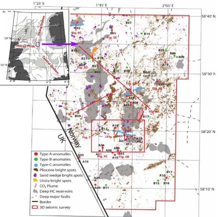
Figure 3.1.1: Map of the Sleipner area in the SVG showing the location of fluid flow manifestations and exploration

type seismic profiles (red lines): bright spots beneath the top of the Utsira Formation (pale green), within the sand

wedge (pale red), beneath the top Pliocene (pale blue), type-A-anomalies (red dots), type-B-anomalies (green dots),

type-C-anomalies (red dots), CO2-plume (rose), deep hydrocarbon reservoirs (grey), deep faults (black lines)

[Karstens, 2015]

(14)

a new approach regarding the environmental risk assessment for sub-seabed storage sites of carbon capture and storage (CCS) projects. ECO

2

was triggered by the activities of several EU supported demonstration projects to store CO

2

at the emergence of fossil fuel power plants into either marine sub-seabed storage sites or onshore deep geological formations. Within the industrial countries CCS is regarded as a key technology to significantly reduce CO

2

emissions from new and existing industrial sources and mitigate the contribution of greenhouse gas emissions to global warming and ocean acidification. In particular the injection into oil-, gas- or water-bearing geological storage sites is regarded as a suitable option for carbon dioxide sequestration on a commercial scale [Rackley, 2010]. ECO

2

conducted a comprehensive offshore field programme at the Norwegian storage sites Sleipner and Snøvit and at several natural CO

2

seepage sites in order to identify potential pathways for CO

2

leakage through the overburden and to monitor and track their fluid flux in the seabed and water column. The key objectives addressed by ECO

2

were to investigate the likelihood of leakage from sub-seabed storage sites, understand the potential effects on benthic ecosystems and finally assess the risk of sub-seabed carbon dioxide storage sites. The objectives were followed by numerous field campaigns, research cruises, laboratory experiments and numerical modelling [ECO

2

, 2015]. As one of the main results the investigations of ECO

2

revealed that a quantitative assessment of CO2 seepage rates and a reliable prediction of seep sites cannot be conducted unless the nature, and in particular the permeability of sub-seabed chimney structures is better constrained.

During his PhD thesis [Karstens, 2015] Jens Karstens of GEOMAR mapped, quantified and interpreted focused fluid conduits in the marine sedimentary basin of the Sleipner area in the North Sea Basin in the exploration type 3D seismic data set ST98M3, acquired by Statoil.

Research on the Sleipner CO

2

storage site has mainly focused on the CO

2

migration within the storage formation [e.g. Chadwick et al., 2009; Arts et al., 2008], while natural fluid manifestations in the overburden have only been reported briefly by Heggland [1997] and Nicoll [2011]. The investigated industrial data cover an area of 2,000 km

²

and were processed with 12.5 m horizontal and ~10 m vertical resolution. Karstens mapped and categorised vertical seismic anomalies (Figure 3.1.1, type-A-anomalies, type-B-anomalies, type-C-anomalies). In total, 46 large-scale vertical seismic anomalies (500–800 m long and 100-1000 m wide) are present in the shallow (> 1000) subsurface of the study area and their appearance assigned to different formation processes (Figure 3.1.1). These seismically-imaged chimneys are considered to be pathways for sedimentary fluid flow, which could act as pathways for CO

2

, if the plume reaches the base of the structures and if their permeability is high enough. The analyses revealed seal- weakening, formation-wide overpressure and the presence of free gas as the requirements to initiate the formation of vertical fluid conduits in the SVG [Karstens & Bendt, 2015].

Similar seismic anomalies have been recognized around the world and are generally associated with vertical fluid flow [e.g. Berndt, 2005; Cartwright et al., 2007; Løseth et al., 2009;

Andresen, 2012; Gay et al., 2012]. The activity of vertical fluid conduits can be associated to blowout-like events, e.g. resulting in pipe structures offshore Nigeria [Løseth et al., 2011] or Norway [Bünz et al., 2003] or fluid flow may be continuous and long-lasting, e.g. chimney structures above North Sea salt diapirs [Hovland and Sommerville, 1985; Granli et al., 1999;

Arntsen et al., 2007]. The shallow subsurface of the Central North Sea is highly affected by

(15)

Cruise

focused area is d while a meter [ beneath seismic compara

We Norway cruise. B were jud data cou would b Site dep Alltoget profiler seismom fracture be comb modelli

Figure 3 Chimney pockmar

e report MSM

d fluid flow.

densely pop few promi [Judd and H h a glacial u

data sugg able to the s

selected the y) and the S

Both structu dged suitab uld not reso be reachabl pended on h

ther we did data to ima meter data e anisotropy bined to a g

ng after th

3.1.2: Seismic y A04 south rk in high-res

Line:

Trace:

Offset:

0.100

0.200

0.300

0.400

0.500

0.600

0.700

0.800

0.900

1.000

1.100

1.200

1.300

1.400

1.500

M63

. The seaflo pulated with inent structu

Hovland, 2 unconformit gest that th

seismic flui

e two prom Scanner poc

ures have b ble for our e

olve if the f le with drill high-resolut

d acquire h age small-s

for velocit y in the subs

geophysical he data hav

c examples fo of the Sleip olution 2D se

oor of the F h pockmark

ures like th 2007]. The

ty less than is shallow id flow struc

minent verti kmark (U.K been imaged xperiments fluid condu ling. Theref tion sub-bot high-resolut cale fractur ty analysis surface [Exl l model of a ve been gro

or pipe struct pner Field. Th

ismic data col

1 20000

A04

Fladen Grou ks. Most of t he Scanner Scanner p n 80 meters gas reserv ctures ident

ical seismic K.) in the So d previously (Figures 3.

uit of A04 c fore, the fin ttom profile tion 2D sei re networks and contro ley et al., 20 a chimney s ound-truthe

tures. The lef he right pane llected during

km

und in the B these pockm pockmark h pockmark e

s below the voir is char tified in the

c fluid flow outhern Vik y with expl .1.2, right an crosscuts th

nal site sele er data, whic ismic data,

in the top olled source

010; Key et structure an d by drillin

ft panel show el shows the g MSM63.

British secto marks are on

have diame mits metha e seafloor [J rged by a

Sleipner ar

w structure king Graben

oration-type nd left). Ho e youngest ection for t ch we colle very high- 20 m of sed e electroma t al., 2012].

nd form the ng. These

ws exploration pipe structur

or west of t nly a few m eters of mor ane, which

Judd et al., vertical flu rea (Figure 3

s A04 (Sle n as study s

e 3D seism owever, the glacial sed the Scanner ected during -resolution

diments, oc agnetic dat All four da

basis for p data will p

n type 3D sei re underlying

9 he Sleipner meters wide, re than 100 is trapped 1994]. 3D uid conduit 3.1.2 left).

eipner area, ites for this mic data and 3D seismic diments and r Pockmark g the cruise.

sub-bottom cean bottom a to assess ata sets will ermeability provide the

ismic data of the Scanner

r , 0 d D t

,

s

d

c

d

k

.

m

s

l

y

e

(16)

steppingstone from interpretation of borehole samples to exploration-type 3D seismic data. This will provide the geophysical database for assessing the permeability of a typical chimney structure. Within the STEMM-CCS project the analysis and interpretation of the borehole results will be augmented with the study of field analogues and numerical simulations.

3.2 Aims of the Cruise

Quantification of focused fluid migration through the sedimentary succession is fundamental for a large number of research themes ranging from the assessment of geological climate controls and slope stability to verify applied question such as where hydrocarbons accumulate and how safe CO

2

storage is [Berndt, 2005]. Within the ECO

2

project we have attempted to assess the integrity of the overburden, but the combination of field studies and numerical simulation has shown clearly that it is not possible to describe fluid migration in a sedimentary basin quantitatively without understanding the role of seismic chimney structures.

The main scientific goals of this project were

a) firstly to constrain the bulk permeability of an existing chimney structure, i.e. to assess the amount of aqueous and gassy fluids that may move through these structures over time.

b) Secondly, we tried to constrain the temporal evolution of fluid migration through pipe structures over time, i.e. do they transport fluids continuously or episodically and if episodically is it likely that CO

2

storage may initiate a new episode of migration.

c) Thirdly, we set out to test the hypothesis that chimney structures in seismic data represent indeed fault networks created by hydro-fracturing and not bulk mobilization of sediments as a diapir or subsidence of sediments in the style of a breccia pipe.

These goals will be met within the STEMM-CCS project by combining geophysical

observations from two scientific cruises by GEOMAR and the National Oceanography Centre,

Southampton with field samples from the Colorado Plateau and numerical simulations. The

cruise proposed here will provide the required borehole samples from inside and outside the

chimney structures and the necessary geophysical data with different frequency content from

high-resolution sub bottom profiler data to P-Cable high-resolution data to upscale the borehole

observations through a nested approach to the existing high-quality exploration-type seismic

data. This will provide the required data set to achieve the three objectives above. These data

will be augmented by ocean bottom seismometer data and controlled-source electro-magnetic

data, which we will collect during the cruise and which will allow us determining if there is

continuously linked fracture permeability inside the chimney structures from directional

differences in the seismic velocities and the electric resistivity, respectively.

(17)

Cruise

4 Figure 4.1 25.05.201 main stud the U.K. s

e report MSM

Narrat (C. Ber

1: Cruise MSM 7 after a port dy area during sector of the N

M63

tive of the C rndt, J. Elge

M63 started f t call in Aberd g Leg 1 was th North Sea.

Cruise er)

from Southam deen from 12.

he Scanner Po

mpton, U.K. o .-18.05.2017 w ockmark, duri

n 29.05.2017 when the geop ing Leg 2 it w

and finished physical equip was the Golden

in Southamp pment was of neye field, bo

11 pton, U.K. on

ffloaded. The

oth located in

(18)

29.4. Saturday

After mobilization of OBEMs and DASI we sailed from Southampton at 17:30. We set off for the study area with a south-easterly breeze.

1.5. Monday

We arrived in the first study area south of the Sleipner Field at 22:00. We carried out releaser tests for both the OBEM and the OBS and ran a sound velocity profile.

2.5. Tuesday

In the early morning from 2 to 5 o’clock we ran several Parasound profiles to inspect if the chimney structure at site A03 reaches the surface sediments as indicated by the low-resolution 3D-seismic data. Unfortunately this is not the case also the secondary target site A04 did not show any evidence for a fluid flow anomaly within the top 30 m that could be reached by RockDrill2. Therefore, we decided to steam to the back-up location in the British sector (Scanner Pockmark). We reached that site at 08:00 and began to deploy the OBIC OBEM’s. After having deployed six OBEM we continued with the deployment of the GEOMAR OBS at 14:00 to allow the OBIC team to have a break. All 17 OBS were deployed by 20:30. Then we fixed a sensor on Merian’s pod drive and carried out a high-voltage test on DASI before deploying the remaining OBEMs starting at 21:30.

3.5. Wednesday

At 03:30 all OBEM were installed at the sea floor and we continued with the deployment of DASI which was up and running by 07:00. For the next two days we acquired CSEM data in good weather (N2-4).

5.5. Friday

Except for a short break to change the battery of the Posidonia receiver on DASI in the evening of the 4.5. the DASI system ran smoothly until we recovered it in the morning of the 5

^th

between 08:00 and 09:00. Then we continued with the recovery of the OBEMs. These were on deck at 14:00. During the afternoon and early evening we deployed the P-Cable system, but there were technical difficulties. Two t-junctions caused leakage and even though the system worked for a short time after everything was deployed, more leakage occurred just before firing up the airguns and everything had to be retrieved. During the night we shot at 10 s intervals into the OBS.

6.5. Saturday

Because of poor weather forecast force 7-8 from Sunday morning, we decided not to try to

deploy the P-Cable system again but continued shooting into the OBS. At 10:00 o’clock we had

to stop to repair one of the pod drives. Afterwards, we continued with shooting the OBS lines but

now also with a 2D streamer and a higher shooting rate in order to produce reverse shot lines and

geometry information in addition to the dedicated OBS shots at 10 s intervals.

(19)

Cruise report MSM63 13

7.5. Sunday

At 08:00 we retrieved the 2D seismic system because the weather deteriorated with up to 6 m high waves. For the following two days we conducted a multibeam survey that covered 2/3 of the study area.

9.5. Tuesday

We started to recover the OBS at 06:00 and managed to retrieve all eighteen instruments by 12:00. Afterwards we redeployed the P-Cable system. The system was up and running by 18:00, but after a few shots leakage in one of the cables occurred and we had to get it back on deck.

Afterwards we re-configured it in 2D mode and at 22:00 we started to acquire 2D seismic data during the night.

10.5. Wednesday

At 08:00 we repaired streamer three in which the connector broke during the night. The system was up an running again within one hour.

11.5. Thursday

In the morning the airgun float collapsed and we had to repair it before continuing shooting 2D seismic lines across the CSEM DASI profiles. At 16:00 we retrieved the 2D seismic system and ran another sound velocity profile for the calibration of the multibeam system, before starting the transit to Aberdeen.

12.5. Friday

We arrived in the prot of Aberdeen at 06:00. All instruments used on leg 1 were demobilized and unloaded by noon. The mobilization of RD2 (rock drill) started at 08:00.

18.5. Thursday

After spending the last 5 days in Aberdeen harbour because of technical problems we sailed from Aberdeen at 19:00. During that time RD2 had have to be demobilized, as the remaining time of the second leg of MSM63 does not allow to drill any cores and demobilize RD2 then in Southampton. Instead we plan to use multibeam, Parasound, CTD and water samples to study the area around the Golden Eye platform. We set off for the study area with sunshine and a south easterly breeze.

19.5. Friday

At about 01:00 we arrived in the study area the Golden Eye platform and started to acquire

Parasound data. At about 13:30 we stopped to measure a CTD profile to measure salinity,

pressure, temperature, oxygen and turbidity and to take water samples for further analyses in the

lab at home. Afterwards we continued the Parasound measurements until 16:15 and did a second

CTD. At about 17:00 we started with a multibeam survey that will image the seafloor in an area

of about 10 by 10 km around the Golden Eye platform.

(20)

20.5. Saturday

We interrupted the multibeam survey to measure the water column with the CTD at three locations around the Golden Eye platform, at about 08:30, 11:30 and 13:15, and one at about 15:00 in the north-western part of the survey area. As the wind got stronger during the night, there is about 2 m of swell.

21.5. Sunday

We finished the multibeam survey at around 03:00 in the night and sailed to the

Scanner pockmark area. We turned on the Parasound until we left the area of study permission at Golden Eye, about 05:30. In the morning we started the mulitbeam survey in the Scanner pockmark area around 08:15. We took two CTD measurements in the early afternoon, one in the Scanner pockmark at the flare and one outside. The wind calmed down again and the sea is very calm.

22.5. Monday

We finished the multibeam survey shortly after midnight and headed back to the Golden Eye platform. Back there, we filled up gaps in the multibeam data until about 08:30. Afterwards, we did 8 CTD measurments (with and without water sampling) and connected them with Parasound profiles. Afterwards we did another multibeam survey in the southwestern part of the study area.

In the evening, we started to measure a grid of Parasound profiles on the eastern side of the platform.

23.5. Tuesday

We finished the Parasound survey around 02:00 in the morning and set off for Southampton.

25.5. Thursday

After about 2 days of transit the pilot entered the vessel around 06:00 and we arrived in the port

of Southampton at 08:00.

(21)

Cruise report MSM63 15

5 Preliminary Results

5.1 Seismic Data Acquisition and Processing (S. Muff)

5.1.1 Method and experiment setup

The aim of the seismic survey was to map the spatial extent of the scanner pockmark. During the cruise an array of two 105/105 in3 GI-Gun's was fired as seismic source for the seismic lines.

Data were recorded with GeoEel digital streamer segments. Fig. 5.1.1 gives an overview upon the seismic 2D lines during Cruise MSM63.

Figure 5.1.1: 2D survey lines of MSM63: Red lines show lines of P2000. Black lines show lines of P3000.

(22)

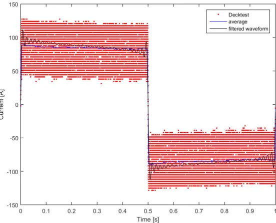
Seismic During Both gu beneath of ~2 m

Each gu injector provide direct q delay of value w bar).

The sho distance gun wa speed. T

c sources this cruise uns were co h. An elonga m, was conne

un had a vo r chamber.

both, the ti quality contr f 5 ms in m was adjusted

ooting interv e of 10.50 -

s fired ever The frequen

two standa onnected to

ated buoy, w ected to the

olume of 21 A gun hyd ime break a rol of the so manual mod d to the appr

val was adju - 15 m in a ry 5 second ncy range of

ard GI-Gun a stringer which stabi stringer by

10 in3, sepa drophone, w and the shap

ource signa de with resp roximated s

usted to 6 s range of ap ds, resulting

f the two-GI

Figu

ns in harmo with the G ilized the gu y two rope lo

arated in 10 which is lo pe of the ne al. The relea pect to the g source depth

seconds for pproximate g in a shot p

I-Gun-array

ure 5.1.2: GI-G

onic mode w GI-Guns han

uns in a ho oops (Fig. 5

05 in3 for t cated insid ear-field sign

ase of the in generator si

h of 2 m an

survey line ly 3.5 – 5 k point distan y is 15 - 500

Gun setup

were operat nging on tw rizontal pos 5.1.2).

the generato e the air b nal for perm njector puls

gnal for all d a gun pre

es P2000, re knots. For s nce of 8.75 0 Hz.

ted as seism wo chains ab

sition at a w

or and 105 bubble, is s

manent mon e was trigg l seismic su essure of 30

esulting in a survey lines – 12.5 m a

mic source.

bout 70 cm water depth

in3 for the upposed to nitoring and gered with a urveys. This 00 psi (210

a shot point s P3000 the at the same . m h

e o d a s 0

t

e

(23)

Cruise report MSM63 17

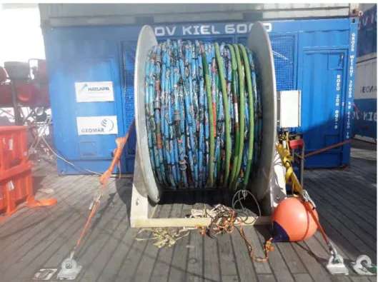
Streamer System

Different configurations in digital streamer length (Geometrics GeoEel streamer segments) were used for recording the seismic signal. Deck geometries, streamer configuration and seismic gun setting for the 2D surveys are illustrated in Fig. 5.1.3. The entire survey P2000 and lines 3 to 10 from survey P3000 were recorded with two oil filled streamer sections (each 12.5 m) with 16 channels. Survey lines two and all lines in between eleven and thirty from survey P3000 were recorded with a 150 m long streamer and 96 channels. The last four streamers of this configuration were solid state. All streamer configurations consisted of a tow cable, one vibro stretch section of 25 m length behind the tow cable the active sections (each 12.5 m) attached behind the stretch zone. The tow cable had a length of 20 m behind the vessel's stern. Each active section contained 8 channels with a hydrophone group spacing of 1.56 m. One AD digitizer module belonged to each active section. These AD digitizer modules are small Linux computers.

Communication between the AD digitizer modules and the recording system in the lab was transmitted via TCP/IP. A repeater was located between the deck cable and the tow cable (Lead- In). The SPSU managed the power supply and communication between the recording system and the AD digitizer modules. Three birds controlled and monitored the streamer depth during the survey with 96 channels. They were attached to the stretch zone, the first and the third streamer segment. A small buoy was connected to the tail swivel of the 2D streamer (Fig. 5.1.4).

Figure 5.1.3: GeoEel streamer segments of 12.5 m length were connected to build up the 2D streamer system.

(24)

Bird Controller

Three Oyo Geospace Bird Remote Units (RUs) were deployed on the streamer. The locations of the birds are listed in Fig. 5.1.4. The RUs have adjustable wings. A bird controller in the seismic lab controlled the RUs. Controller and RUs communicate via communication coils nested within the streamer. A twisted pair wire within the deck cable connects controller and coils. Designated streamer depth was 2 m in accordance with good weather conditions and low swell noise. The RUs thus forced the streamer to the chosen depth by adjusting the wing angles accordingly. The birds were deployed at the beginning of a survey but no scanning of the birds was carried out during the survey because bird scans caused false triggers. However, the birds worked very reliably and kept the streamer at the designated depth.

Figure 5.1.4: Geometry and streamer configuration of the 2D seismic surveys.

(25)

Cruise report MSM63 19

Data Acquisition Systems

Data were recorded with acquisition software provided by Geometrics. The analogue signal was digitized with 2 kHz. The seismic data were recorded as multiplexed SEG-D. Recording length was 6 (P2000) and 5 seconds (P3000). One file with all channels within the streamer configuration was generated per shot. The corresponding Shotlog reports shot number and time information contained in the RMC string. The acquisition PC allowed online quality control by displaying shot gathers, a noise window, and the frequency spectrum of each shot. The cycle time of the shots were displayed as well. The software also allows online NMO-Correction and stacking of data for displaying stacked sections. The vessel's GPS was simultaneously logged in RMC string and logged time and position information.

Trigger Unit

A long shot was used as gun controller. The injector was triggered with a delay of 5 ms in manual mode. From seismic data analyses we determined a total delay of 18 ms for lines one to four of survey P2000 and all other lines a delay of 20 ms between triggering and real shooting time. No direct quality control of the source signal was carried out.

Processing

On-board processing included geometry calculations, delay calculations and source and receiver depth control. A ghost effect in the seismic data was not detected. The processing was performed with the Seismic Unix software. The source-receiver locations were binned on a grid with 1.5625 m by 1.5625 m cells. Survey lines P2000 were bandpass-filtered with a low-cut ramp of 55 – 65 Hz and a high-cut ramp of 350 - 500 Hz to suppress a strong bubble pulse overprint. Survey lines P3000 were filtered with bandpass corner frequencies of 25, 45, 420, 500 Hz. An NMO correction (with a constant velocity of 1488.08 m/s calculated from CTD measurements) was than applied and the data stacked. The stack was migrated with a 2D Stolt algorithm (1500 m/s constant velocity model).

5.1.2 Initial Results (C. Boettner)

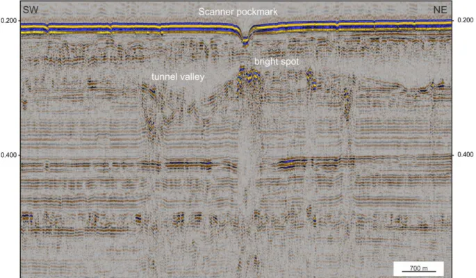
Preliminary analysis of 2D seismic lines show the overall shape of the sedimentary succession underneath the Scanner pockmark. The seismic image (see Figure 5.1.5) is centered around the Scanner pockmark and show it as a ~ 180 m wide and ~16 m deep depression at the seafloor.

The sedimentary succession is well imaged by the high-resolution 2D seismic data. The Nordland formation is clearly visible as well-stratified sediments. The multiple of the seafloor is distorting the image at ~ 440 ms.

Between the seafloor and the well-stratified sediments of the Nordland formation (200-350

ms TWT) clear indication for several stage of deposition and erosion are visible. A characteristic

tunnel valley with steep flanks and several phases of deposition and erosion is located SW of the

Scanner pockmark. The 2D seismic data provides higher resolution and quality than the pre-

(26)

existing 3D industry seismic data for the upper 500 ms TWT. Especially the different stages of glacial deposition and erosion can be untangled and further interpreted with the data.

A chimney-type anomaly is visible underneath the Scanner pockmark. However, our data does not enable a clear distinction between seismic artifact and real geological fluid conduit. At the topmost extent of the blanking zone, a bright spots are visible. Although the bright spots show amplitude increase by a magnitude, a single flat spot is not visible. A single flat spot would indicate large amounts of free gas and/or a single reservoir within the sedimentary succession.

However, we can state that this gas reservoir underneath the Scanner pockmark is likely the source region of the flares emerging from the center of the pockmark. A conduit or fracture network between the bright spots and the Scanner pockmark is undetectable as only one wiggle trace shows anomalous behavior.

5.2 OBS Experiments (B. Schramm)

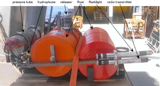
The Ocean Bottom Seismometer (OBS) consists of four floats, which are connected to a frame and is generally equipped with a three-component seismometer, a hydrophone and a data recorder encased in a high-pressure tube (Fig. 5.2.1). All sensors are connected to the recording unit and continuously record the incoming signals. The system itself floats at the sea surface, so in order to deploy the device on the ocean bottom a weight is mounted to the frame and attached to a so-called releaser. This releaser has an acoustic communication unit, which can be addressed from the ship in order to disconnect the weight after the experiment. The OBS will then ascend to the surface and can be recovered. A flashlight, radio transmitter and a flag are attached to the

Figure 5.1.5: Seismic image of the Scanner pockmark

(27)

Cruise report MSM63 21

frame to increase the visibility of the OBS and to facilitate an easy and quick recovery. While the OBS continuously records seismic signals an additional data logger on board records the corresponding shot times and is used to correlate the results at a later stage of data processing.

The data recorders need to be programmed before the deployment of the system. The sample rate of the OBS recorders was set to 500 Hz, while the time logger had a sample rate of 1000 Hz.

The gain of the input channels was set to 15 for the three geophone components and to 7 for the hydrophones. Initial tests showed some problems with the recording unit of OBS 18, so that the gain for the geophone components was increased to 31.

Each recorder was equipped with 5 GB storage space (either one 2 GB and three 1 GB or two 2 GB and two 1 GB flash memory cards). The exact recording parameters for the deployments can be found in Appendix B (OBS protocols). The recording units were synchronized with the GPS signal both before and after the recording period to correct for any time shifts within the logger’s internal clock.

A total of 18 OBS were deployed around the chimney on May the 1

^st

2017 (Fig.5.2.2). The water depth varied between 153 and 169 m. Afterwards, the airgun was deployed and six profiles (P1001 – P1006) crossing the OBS were shot for 10 hours. The shot interval was 10 s with two GI-guns (Appendix C). In addition, a streamer was deployed on the following day and the shot interval was reduced to 6 s (P2001-P2013). Ring profiles could not be achieved due to bad weather conditions.

Figure 5.2.1: GEOMAR Ocean Bottom Seismometer (OBS)

(28)

The well as

All immedi recorder synchro failed du

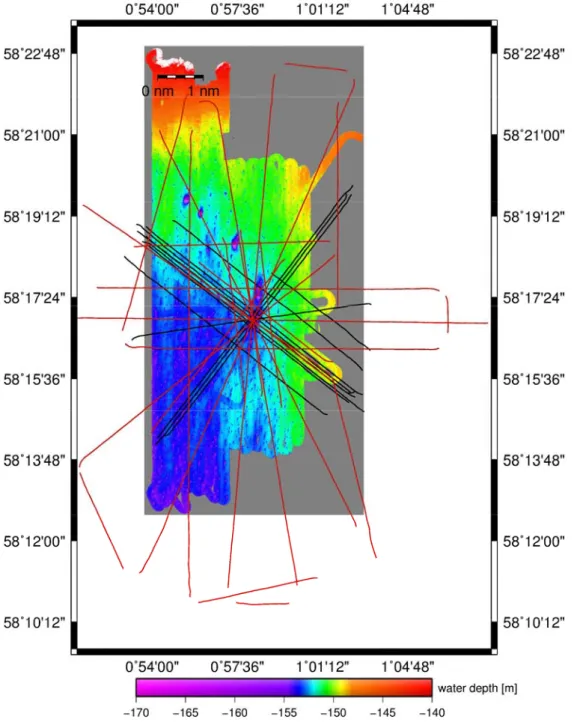
main target to support f 18 OBS w ately read rs, because onized, but uring record

Figure 5.2.

Black lines

t of these p further 2D a were recove and copied the instrum copying of ding.

2: Bathymetr show profiles

profiles was and 3D seism ered succes d to a proc ments went

f the data f

ric overview s P1000 to P20

to provide mic analyse ssfully on cessing un

low on bat failed. On

map of the 000. The red s

e velocity in es of the inv May the 9 it. Synchro ttery during OBS 18, tw

seismic surv square is disp

nformation vestigation a

9

^th

and the onization fa g the operat wo of the g

ey during the laying the OB

for 3D tom area.

e collected ailed with tion. OBS 0

geophone c

e OBS opera BS positions.

mography as

data were two of the 04 could be components

ation.

s

e

s

(29)

Cruise

All d control GEOMA

5.3 5.3.1 The dee deep-tow neutrall respons Vulcan instrum conduct on the frequen seafloor layers. F MSM63

e report MSM

data were co showed pr AR (Fig. 5.2

Contro (R. Geh Introd ep-towed a w cable. D y-buoyant a e of the se

receivers ments. The a tivity (or re conductivi ncies. The i

r and is, th Figures 5.3 3 cruise. Fig

Figu M63

opied and co romising da

2.3).

olled Sourc hrmann, B.

uction to D ctive sourc DASI is de antenna at l afloor is th [Constable amplitude an sistivity - th ity structur instrument herefore, sen

.1 and 5.3.2 gure 5.3.3 sh

ure 5.2.3: This

onverted to ata, but deta

ce Electrom Pitcairn) DASI and V

e instrumen esigned to t

low frequen hen measure

e et al., 2 nd phase of he inverse o re is then array is sen nsitive to t 2 show the hows the in

figure shows

SEG-Y/ PA ailed proce

magnetic Su

Vulcan nt (DASI) transmit el ncies that pe

ed and reco 2016] and f the measu of the condu

inferred f nsitive to b the contrast schematic s nstrument du

the X compo

ASSCAL fi ssing will b

urveys

is powered lectromagne enetrates the orded by tw ocean bo ured EM re

uctivity) of from the r bulk change

t between r setup of the uring deploy

onent of OBS 0

les on board be carried o

d from the etic (EM) s

e seafloor [ wo towed th

ottom elect sponse is re f the seafloo responses m

es in electr resistive an e STEMM-C

yment.

01, 02, 03 and

d. A first qu out after th

ship via a signals from [Sinha, 1989

hree-axis el tromagnetic elated to th or. Further i measured a ric conducti nd conducti

CCS survey

d 09

23 uick quality he cruise at

conducting m a towed 9]. The EM lectric field c (OBEM) he electrical information at different ivity in the ve seafloor y during the y

t

g

d

M

d

)

l

n

t

e

r

e

(30)

Figure 5.3.2: Details on the DASI and Vulcan dimension (scale in metres) setup for the STEMM-CCS survey.

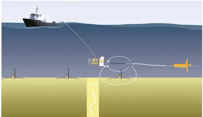
Figure 5.3.1: Sketch of the University of Southampton towed CSEM system: DASI [Sinha, 1989] towing

the dipole transmitting antenna array (white lines represent current streamlines generated by the antenna),

the three-axis electric field Vulcan receiver [Constable et et al., 2016] and three-axis ocean bottom electric

field receivers (OBIC). Figure adapted from Weitemeyer (pers. communication)

(31)

Cruise report MSM63 25

For this experiment, the planned EM survey gridlines (shown below which is superimposed with the location of the deployed Ocean Bottom Electric (OBE) field receivers and the amplitude of the glacial unconformity reflections from seismic data, courtesy of PGS) is indicated in the Figure 5.3.4.

Figure 5.3.4: This figure shows the superimposed plot of the locations of deployed OBEM and seismicreflecteddata(data courtesy of PGS) and EM survey lines. The X & Y axes show UTM coordinates.

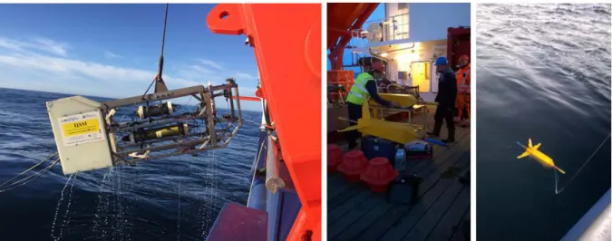
Figure 5.3.3: a (left), b (centre) and c (right) show the DASI transmitter deployed off the aft of FS Merian and

the towed EM receivers (Vulcans) used for this survey.

(32)

5.3.2 Ocean Bottom Electro-Magnetic (OBEM) Receivers

UK based OBIC (Ocean Bottom Instrumentation Consortium) supplied 14 OBEM (Ocean Bottom Electro-Magnetic) receivers for this STEMM_CCS work package. These instruments are based on the LCHEAPO platform and the LC2000 data logger developed by Scripps Institution of Oceanography, USA. All of the instruments were equipped with two orthogonal horizontal 12m electrode dipoles, six were equipped with a vertical 1.5m dipole in addition. Red farings are used to reduce the strumming on the pole.

All instruments were equipped with a burn-wire release system and light, VHF radio, and high-visibility flag to aid with recovery. All of the acoustic releases were tested prior to deployment using a basket lowered from the ships CTD winch.

5.3.2.1 OBEM Deployments

The instruments were lowered to 12 m from the seabed using the ship’s winch, run through a pulley block on crane 3. They were then released to freefall the remaining distance using an acoustic release supplied and operated by the ship’s crew. The position of release was logged by the IxBlue Posidonia receiver. After the initial setup of the winch and release system, each deployment took between 40 minutes and one hour to complete. The instruments were deployed in two shifts on the 2

^nd

and 3

^rd

May 2017.

5.3.2.2 Recoveries

All the OBEM recoveries were completed on 5

^th

May 2017. All acoustic communication was done using the ship’s hull mounted transducer which worked well for all recoveries. The fast rescue boat was used to assist in locating and retrieving the instruments which sped up the time taken to position the ship and crane each instrument on board. Each instrument took between 15 and 20 minutes to recover and partially disassemble.

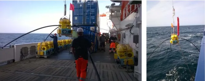
Figure 5.3.5: The OBEM deployment without and with vertical electrode arm off Maria S. Merian’s starboard side.

(33)

Cruise report MSM63 27

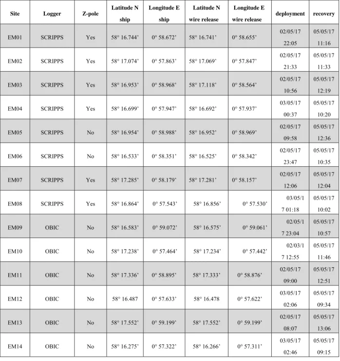
Table 1: Summary of OBEM deployments on MSM63. All positions are the ship position at time of deployment.

Site Logger Z-pole Latitude N

ship

Longitude E ship

Latitude N wire release

Longitude E wire release

deployment recovery

EM01 SCRIPPS Yes 58° 16.744’ 0° 58.672’ 58° 16.741’ 0° 58.655’ 02/05/17 22:05

05/05/17 11:16 EM02 SCRIPPS Yes 58° 17.074’ 0° 57.863’ 58° 17.069’ 0° 57.847’ 02/05/17