doi: 10.4208/cicp.190313.010813a February 2014
Phase Field Models Versus Parametric Front Tracking Methods: Are They Accurate and Computationally Efficient?
John W. Barrett1, Harald Garcke2,∗and Robert N ¨urnberg1
1Department of Mathematics, Imperial College London, London, SW7 2AZ, UK.
2Fakult¨at f ¨ur Mathematik, Universit¨at Regensburg, 93040 Regensburg, Germany.
Received 19 March 2013; Accepted (in revised version) 1 August 2013 Available online 27 September 2013
Abstract. We critically compare the practicality and accuracy of numerical approxima- tions of phase field models and sharp interface models of solidification. Here we focus on Stefan problems, and their quasi-static variants, with applications to crystal growth.
New approaches with a high mesh quality for the parametric approximations of the re- sulting free boundary problems and new stable discretizations of the anisotropic phase field system are taken into account in a comparison involving benchmark problems based on exact solutions of the free boundary problem.
AMS subject classifications: 35K55, 35R35, 35R37, 53C44, 65M12, 65M50, 65M60, 74E10, 74E15, 74N20, 80A22, 82C26
Key words: Phase field models, parametric sharp interface methods, Stefan problem, anisotropy, solidification, crystal growth, numerical simulations, benchmark problems.
1 Introduction
The solidification of a liquid or the melting of a solid lead to complex free boundary problems involving many different physical effects. For example, latent heat is set free at the interface and a competition between surface energy and diffusion leads to insta- bilities like the Mullins-Sekerka instability. The resulting model is a Stefan problem with boundary conditions taking surface energy effects and kinetic effects at the interface into account, see e.g. [37, 51]. Crystals forming in an undercooled melt lead to very complex
∗Corresponding author. Email addresses: j.barrett@imperial.ac.uk (J. W. Barrett), harald.garcke@
mathematik.uni-regensburg.de(H. Garcke),robert.nurnberg@imperial.ac.uk(R. N ¨urnberg)
patterns and, in particular, dendritic growth can be observed since the growth is typically diffusion limited, see [20].
The numerical simulation of time-dependent Stefan problems, or variants of it, is a formidable task since the evolving free boundary has to be computed. Hence, di- rect front tracking type numerical methods need to adequately capture the geometry of the interface and to evolve the interface approximation, often with a coupling to other physical fields. This coupling, in particular, represents a significant initial hurdle to- wards obtaining practical implementations, and thus numerical simulations for the prob- lem at hand. Examples of the implementation of such direct methods can be found in e.g. [1, 3, 6, 13, 53, 54, 57, 72–75, 81, 86].
A further drawback of direct front tracking methods has been the inability of most direct methods to deal with so-called mesh effects, or to prevent them altogether. When a discrete approximation of an interface, for example a polygonal curve in the plane, evolves in time, then in general it is possible for the approximation to deteriorate or to break down. Examples of such pathologies are self-crossings and vertex coalescence.
While for simple isotropic problems in the plane these issues can be dealt with, for ex- ample by frequent remeshings or by using clever formulations that only allow equidis- tributed approximations, see e.g. [57, 81], until very recently there has been no remedy for fully anisotropic problems in two and three space dimensions.
However, building on their work for isotropic problems in [8, 9, 11], the present au- thors recently introduced stable parametric finite element schemes for the direct approx- imation of anisotropic geometric evolution equations in [10, 12], for which good mesh properties can be guaranteed. In particular, even for the simulation of interface evolu- tions in the presence of strong anisotropies, no remeshing or redistribution of vertices is needed in practice. These schemes, in which only the interface without a coupling to bulk quantities is modelled, have been extended to approximations of the Stefan problem with fully anisotropic Gibbs-Thomson law and kinetic undercooling in [13]. The novel method from [13] can be shown to be stable and to have good mesh properties. We remark that these approaches extend earlier ideas from [39, 73, 74]. Here we recall the pioneering work of Schmidt [73, 74], where the full Stefan problem in three dimensions was solved within a sharp interface framework for the first time.
Phase field methods are an alternative approach to solve solidification phenomena in the framework of continuum modelling. In phase field approaches a new non-conserved order parameter ϕis introduced, which in the two phases is close to two different pre- scribed values and which smoothly changes its value across a small diffuse interfacial re- gion. A parabolic partial differential equation forϕis then coupled to an energy balance, which results in a diffusion equation for the temperature taking latent heat effects into account. We refer to [27, 36, 59, 70, 83] and to the five review articles [25, 33, 62, 77, 79] for further details. In particular, it can be shown that solutions to the phase field equations converge to classical sharp interface problems, see e.g. [2, 28, 29, 78] and the references therein.
The popularity of phase field methods, often also called diffuse interface methods,
can be explained by two characteristic features that they share with the level set method, which is another sharp interface computational tool. Firstly, phase field methods nat- urally allow for changes of topology. And secondly, computing simulations for phase field models only requires the solution of partial differential equations on standard Carte- sian domains. The fact that these can usually be implemented and solved in a relatively straightforward way makes the phase field method particularly appealing. For complete- ness we mention that it is also possible to include topological changes in front tracking methods, even though topological changes represent a singularity for the sharp interface model itself. Here one possible approach is to draw up a list of heuristic criteria which trigger a topological change. In contrast to diffuse interface methods, this gives some active control over the topological changes; see e.g. [26, 54]. An alternative approach is to employ a diffuse interface method as a computational tool within a front tracking algo- rithm, which allows the algorithm to integrate through topological changes. An example for such a coupling in the level set context can be found in [68].
It is the aim of this article to investigate the practical merits of phase field models compared to the recently introduced sharp interface algorithm for the approximation of Stefan problems from [13], see also [14, 15], in the absence of topological changes. Of particular interest will be the relative accuracy of the two methods, in situations where a true solution to the sharp interface problem is known. In a phase field simulation the observed error is made up of contributions from
• the asymptotic error,
• the spatial and temporal discretization errors,
• rounding errors and solver tolerances.
Here the asymptotic error is induced by the choice of interfacial parameter ε>0. In general one can formally show that the asymptotic error converges to zero asε→0, see e.g. [27]. For certain phase field models and under certain conditions it can be rigorously shown that the asymptotic error vanishes as ε→0, see e.g. [29]. In computations for sharp interface approximations, on the other hand, the observed error is made up of the latter two contributions only, i.e. of discretization and rounding errors. A disadvantage of phase field models is that the resulting PDEs become stiff for decreasingε, leading to a requirement for very fine spatial and temporal discretizations. Hence it becomes compu- tationally challenging to produce very accurate phase field simulations. In any case, the available computational resources will often set a limit on the smallest interfacial param- eterεthat one can compute for. Hence another aspect that needs to be taken into account in an objective comparison between phase field simulations and sharp interface approx- imations is the overall CPU time that is needed to obtain the results. While it can often be formally shown that phase field computations can attain an arbitrarily high accuracy, the existing limitations on computer hardware often mean that in practice very fine com- putations cannot be performed. In addition, as discussed in [55], the early computational approaches were limited as they could only be used in the presence of interfacial kinetics
in the Gibbs-Thomson law.
Historically these limitations of the phase field model have long been known, and as a result a different underlying interpretation of the model, the so-called “thin interface limit”, has been introduced and analyzed by Karma and Rappel [55, 56]. Their approach made it possible to do efficient computations with a smaller capillary length to inter- face thickness ratio, and to study the physically relevant case of small or zero kinetic coefficients. Later the findings of Karma and Rappel were reinterpreted as second order convergence with respect to the interfacial thickness, see [4,34,47]. Of course, one can ask the question whether phase field models, in their own right, already represent a correct description of phase transition phenomena, rather than just being an approximation to a free boundary problem. In this context, though, one has to decide what value should be chosen for the interfacial parameter. For models of solidification the true length scale of the real-world interfacial region between the two phases is accepted to be orders of mag- nitude smaller than what is currently (and in the foreseeable future) computable with phase field models. In that sense sharp interface models are currently better approxima- tions of the true physics. In conclusion we stress that both phase field models and sharp interface models are continuum approximations of real phenomena. However, in this paper we view the presented phase field models as approximations of the sharp interface limit, to which they converge asε→0. This enables us to objectively compare numerical solutions within the two frameworks.
The first successful phase field computations of dendritic growth were performed by Kobayashi [58], and his computations demonstrated the importance of anisotropy for dendritic growth. Since then many successful improvements with respect to numerical simulations have appeared in the literature. We refer to [43, 55, 65, 71, 84] and the refer- ences therein.
Finally, we would like to mention work on the numerical analysis of phase field and sharp interface approaches. Numerical analysis of discretizations of phase field models can be found in e.g. [18,31,35,45,46,60,85]. Numerical analysis of discretizations of sharp interface models can be found in [13, 15, 82]. We also remark that level set methods are another possible way to solve Stefan problems and related free boundary problems. We refer to [69, 76] for more details on how the level set method can be used to solve free boundary problems.
The remainder of the paper is organized as follows. In Section 2 we state the sharp interface formulation of the two phase Stefan problem with kinetic undercooling and an anisotropic Gibbs-Thomson law. In Section 3 we state the corresponding phase field model and recall the finite element algorithms from [17]. In Section 4 we numerically compare the sharp interface method from [13] with the phase field algorithms from Sec- tion 3 for some isotropic benchmark problems with known true solutions. Computations for a phase field model with a correction term, for which a second order convergence property can formally be shown, are presented in Section 4.3. Finally, we compare the sharp interface and phase field methods for a variety of anisotropic model problems in Section 5.
2 Sharp interface problem
In this paper we concentrate on interfacial problems in materials science in which one driving force is due to capillary effects. In applications the interface often separates a solid and a liquid phase, say, or a solid phase and a gas phase. LetΓ(t)⊂Rd, d=2,3, denote this sharp interface. Then the surface energy ofΓ(t)is defined as
Z
Γ(t)γ(n)ds, (2.1)
where n denotes the unit normal of Γ(t), and where the anisotropic density function γ:Rd→R≥0withγ∈C2(Rd\{0})∩C(Rd)is assumed to be absolutely homogeneous of degree one, i.e.
γ(λp) =|λ|γ(p) ∀ p∈Rd,∀λ∈R ⇒ γ′(p).p=γ(p) ∀ p∈Rd\{0},
withγ′denoting the gradient ofγ. For all the considerations in this paper we assume that γis of the class of anisotropies first introduced by the authors in [10, 12]; see also [13, 17].
Relevant for our considerations is the first variation,−κγ, of (2.1), which can be com- puted as
κγ:=−∇s.γ′(n);
where∇s. is the tangential divergence ofΓ, see e.g. [12, 13, 32]. Note thatκγreduces toκ, the sum of the principal curvatures ofΓ, in the isotropic case, i.e. whenγsatisfies
γ(p) =|p| ∀ p∈Rd. (2.2)
2.1 Stefan problem
Then the full Stefan problem we want to consider in this paper is given as follows, where Ω⊂Rdis a given fixed domain with boundary∂Ωand outer normalν. Findu:Ω×[0,T]→ Rand the interface(Γ(t))t∈[0,T]such that for allt∈(0,T]the following conditions hold:
ϑut−K−∆u=0 inΩ−(t), ϑut−K+∆u=0 inΩ+(t), (2.3a)
K∂u∂n
Γ(t)
=−λV onΓ(t), (2.3b)
ρV
β(n)=ακγ−au onΓ(t), (2.3c)
∂u
∂ν=0 on∂NΩ, u=uD on∂DΩ, (2.3d)
Γ(0) =Γ0, ϑu(·,0) =ϑu0 inΩ. (2.3e)
In the above u denotes the deviation from the melting temperature TM, i.e. TM is the melting temperature for a planar interface. In addition, Ω−(t)⊂Ωis the solid region,
with boundaryΓ(t) =∂Ω−(t), so that the liquid region is given byΩ+(t):=Ω\Ω−(t). Moreover, here and throughout this paper, for a quantity v defined on Ω, we use the shorthand notationsv−:=v|Ω− andv+:=v|Ω+. The parametersϑ≥0,λ>0,ρ≥0,α>0, a>0 are assumed to be constant, while K>0 is assumed to be constant in each phase.
The mobility coefficientβ:Rd→R≥0is assumed to satisfyβ(p)>0 for allp6=0 and to be positively homogeneous of degree one. We note that in the isotropic case (2.2) it is often also assumed that
β(p) =|p| ∀ p∈Rd ⇒ β(n) =1. (2.4) In addition[K∂u∂n]Γ(t)(z):=(K+∂u∂n+−K−∂u∂n−)(z)for allz∈Γ(t), andVis the velocity ofΓ(t) in the direction of its normal n, which from now on we assume is pointing intoΩ+(t). Finally,∂Ω=∂NΩ∪∂DΩwith∂NΩ∩∂DΩ=∅,uD∈R≤0is the applied supercooling at the boundary, andΓ0⊂Ωandu0:Ω→Rare given initial data. Here we use the convention thatuD=0 if∂Ω=∂NΩ.
The model (2.3) can be derived for example within the theory of rational thermody- namics and we refer to [50] for details. We remark that a derivation from thermodynamics would lead to the identitya=Tλ
M. We note that (2.3b) is the well-known Stefan condition, while (2.3c) is the Gibbs-Thomson condition, with kinetic undercooling ifρ>0. The case ϑ>0, ρ>0, α>0 leads to the Stefan problem with the Gibbs-Thomson law and kinetic undercooling. In some models in the literature, see e.g. [61], the kinetic undercooling is set to zero, i.e. ρ=0. Settingϑ=ρ=0 but keeping α>0 leads to the Mullins-Sekerka problem with the Gibbs-Thomson law, see [64].
We recall from [13] that for a solutionuandΓto (2.3) it can be shown that the follow- ing equality holds
d
dtF(Γ,u) =−(K∇u,∇u)−λρa
Z
Γ(t)
V2
β(n)ds≤0, (2.5) where
F(Γ,u):=ϑ
2|u−uD|20+λα a
Z
Γ(t)γ(n)ds−λuD|Ω+(t)| (2.6) and where(·,·)denotes theL2-inner product overΩ, with the corresponding norm given by|·|0, and where|Ω+(t)|:=R
Ω+(t)1 dx.
2.2 Parametric method PFEM
Traditional front tracking methods for sharp interface problems had a major drawback, in that the meshes used to describe the interface seriously deteriorated during the evo- lution. In addition, introducing mesh smoothing during the evolution is difficult, see e.g. the discussion in [74]. For interfaces in the plane it is possible to formulate a non- trivial method such that mesh points are nearly equally distributed during the evolution, see [52, 63]. The present authors introduced a novel parametric finite element method
for problems involving curves and surfaces evolving in time, which has a simple varia- tional structure and which leads to good mesh properties, see [8, 9, 11]. In fact, for curves a semi-discrete variant leads to equally distributed mesh points in the isotropic case, while in the general anisotropic setting equidistribution with respect to some anisotropic weight function is obtained, see [10]. For surfaces the resulting meshes have also good properties, which in the isotropic case can be explained by using ideas from conformal geometry. In particular, no remeshing is needed during the evolution, even in the gen- eral anisotropic situation. An example triangulation obtained during the simulation of dendritic growth in three space dimensions can be seen in Fig. 21, below. In addition, as the mesh for the parameterization of the interface is decoupled from the bulk mesh, no deformation of the bulk mesh is required in order to contain the interface at predefined locations on it.
The novel and stable parametric finite element approximation of (2.3) in the case K+=K−>0 has been introduced by the present authors in [13], and this scheme has been extended to the more general caseK±≥0 in [15]. Throughout this paper we will refer to these variants as PFEM. The algorithm PFEM features the discretization param- etershΓ, hf, hc and τ. HerehΓ refers to the fineness of the triangulated approximation ofΓ(t), for which isoparametric piecewise linear finite elements are employed. In par- ticular, a simple mesh refinement strategy allows for the natural growth of the interface, i.e. elements of the triangulated approximation ofΓ(t)are refined when they become too large. Moreover, the temperature in the bulk is approximated with standard continuous piecewise linear finite elements, and hf and hc refer to bulk mesh parameters for fine regions close to the interface and coarser regions far away from it. For all the computa- tions presented in this paper we fixhc=8hf and, unless stated otherwise, we lethf≈hΓ. Finally,τdenotes a uniform time step size. The linear discrete systems of equations are solved with preconditioned conjugate gradient solvers of suitable Schur complement for- mulations. We refer to [13, 15] for more details. As indicated earlier, no remeshing of the discrete interface is necessary for the scheme PFEM, and all the numerical results pre- sented in this paper for this scheme are performed without any redistribution of mesh points.
3 Phase field model
We now state the phase field model that we are going to consider in this paper. To this end, forp∈Rd, let
A(p) =12|γ(p)|2 ⇒ A′(p) =
(γ(p)γ′(p), p6=0,
0, p=0,
and define
µ(p) =
γ(p)
β(p), p6=0,
¯
µ, p=0,
(3.1)
where ¯µ∈R>0is a constant satisfying minp6=0γ(p)
β(p)≤µ¯≤maxp6=0γ(p) β(p).
Moreover, let ϕ:Ω×(0,T)→R be the phase field variable, so that the sets{x∈Ω:
±ϕ(x,t)>0}are approximations toΩ±(t), with the zero level set ofϕ(·,t)approximating the interfaceΓ(t). On introducing the small interfacial parameterε>0, it can be shown
that 1
cΨEε(ϕ)≈
Z
Γγ(n)ds, forεsufficiently small, where
Eε(ϕ):=
Z
Ω ε
2|γ(∇ϕ)|2+ε−1Ψ(ϕ)dx with cΨ:=
Z 1
−1
q
2Ψ(s)ds. (3.2) HereΨ:R→[0,∞]is a double well potential, which we assume to be symmetric and to have its global minima at±1. The canonical example is
Ψ(s):=14(s2−1)2 ⇒ Ψ′(s) =s3−s and cΨ=13232. (3.3) Another possibility is to choose
Ψ(s):= (1
2 1−s2, |s| ≤1,
∞, |s|>1, ⇒ cΨ=π2; (3.4)
see e.g. [23, 24, 42, 43]. Clearly the obstacle potential (3.4), which in contrast to the smooth quartic potential (3.3) forces ϕto stay within the interval[−1,1], is not differentiable at
±1. Hence, whenever we writeΨ′(s) in the case (3.4) in this paper, we mean that the expression holds only for|s|<1, and that in general a variational inequality needs to be employed.
Our phase field model for (2.3) is then given by the coupled system
ϑwt+λ̺(ϕ)ϕt−∇.(b(ϕ)∇w) =0 in ΩT:=Ω×(0,T), (3.5a)
w=uD on ∂DΩ×(0,T), (3.5b)
b(ϕ)∂w
∂ν =0 on ∂NΩ×(0,T), (3.5c)
ϑw(·,0) =ϑw0 in Ω, (3.5d)
with cΨa
α̺(ϕ)w=ερ
αµ(∇ϕ)ϕt−ε∇.A′(∇ϕ)+ε−1Ψ′(ϕ) in ΩT, (3.6a)
∂ϕ
∂ν =0 on ∂Ω×(0,T), (3.6b)
ϕ(·,0) =ϕ0 in Ω, (3.6c)
where
b(s) =12(1+s)K++12(1−s)K−, and where the function̺∈C1(R)is such that
̺(s)≥0 ∀s∈[−1,1], Z 1
−1̺(y)dy=1 and P(s):=
Z s
−1̺(y)dy. (3.7) We note that P, which is a monotonically increasing function over the interval[−1,1]with P(−1) =0 and P(1) =1, is often called the interpolation function. In this paper, we follow the convention from [43], where̺=P′ is called the shape function. Possible choices of̺ that will be considered in this paper are
(i) ̺(s) =12, (ii) ̺(s) =12(1−s), (iii) ̺(s) =1516(s2−1)2, (iv) ̺(s) =34(1−s2). (3.8) More details on interpolation functions P, respectively shape functions̺, can be found in e.g. [30, 47, 83]. In particular, if one also assumes that̺is symmetric, i.e.
̺(s) =̺(−s) ∀s∈R, (3.9a)
and that
̺(1) =̺(−1) =0, (3.9b)
then a faster rate of convergence of the phase field model to the sharp interface limit, as ε→0, can be shown in the isotropic case (2.2), (2.4) on replacingρin (3.6a) with the first order correction
b
ρ:=ρ+ερ1, (3.10)
whereρ1is defined in (4.7) in Section 4.3, below. The condition (3.9b) is one motivation for the latter two choices in (3.8), with the choice (3.8)(iv) also satisfying the stronger condition (4.9), below, for the quartic potential (3.3). An error analysis for a fully discrete approximation of the phase field model (3.5), (3.6) with the quartic potential (3.3) and the shape function (3.8)(i) in the isotropic case (2.2), (2.4) with∂NΩ=∂Ω andK+=K−>0 has been performed in [45]. These authors also show convergence of the phase field discretizations to the underlying sharp interface problem as ε,h,τ→0, where h and τ denote the discretization parameters in space and time, respectively. However, to our knowledge, no convergence rates are known for the convergence of discretizations of the phase field model to the sharp interface problem (2.3). Here we recall that for the much simpler situation of planar curvature flow, as the sharp interface limit of the isotropic Allen-Cahn equation, such convergence rates have been obtained in [67]. In particular, it can be shown that the zero level sets of discretizations of
ε ϕt=ε∆ϕ−ε−1Ψ′(ϕ)
for the obstacle potential (3.4) converge withO(ε)to the sharp interface limit moving by V=κif
τ=O(h2) =O(ε4). (3.11)
While no such result is known for the full phase field model (3.5), (3.6) even in the isotropic setting, it is natural to expect constraints of the form (3.11) in order to observe O(ε)in practice.
We remark that the phase field analogue of the sharp interface energy identity (2.5) is given by the formal energy bound
d
dtFε(ϕ,w) =−(b(ϕ)∇w,∇w)−ελρa c1
Ψ µ(∇ϕ),(ϕt)2≤0 (3.12) for the phase field model (3.5), (3.6), where
Fε(ϕ,w):=ϑ
2|w−uD|20+λα a
1
cΨEε(ϕ)−λuD
Z
ΩP(ϕ)dx. (3.13) Phase field models that satisfy such an inequality, in analogy to the sharp interface energy identity (2.5), are often called thermodynamically consistent, see [47, 70, 83].
3.1 Phase field methods PFobs-FEM and PFqua-FEM
Unconditionally stable, fully practical finite element approximations of (3.5), (3.6) with either (3.3) or (3.4) have been introduced by the authors in [17]. Here stable means that they satisfy a discrete analogue of the formal energy bound (3.12). Throughout this paper we will refer to the approximations from [17] for (3.3) and (3.4) as PFqua-FEM and PFobs- FEM, respectively, where the inclusion of a subscript refers to the choice of shape function in (3.8), e.g. PFobs(i)-FEM. We recall from [17] that a side effect of the interpolation function P in (3.13) is that the function
G(s) =α(acΨε)−1Ψ(s)−uDP(s)
need no longer have local minima ats=±1 if uD6=0. This can result, for example, in undesired, artificial boundary layers for strong supercoolings, i.e. when−uDis large. For the smooth potentialΨ from (3.3), sufficient conditions fors=±1 to be local minimum points ofG(s)are
̺(±1) =̺′(±1) =0, (3.14) which is evidently satisfied by (3.8)(iii). In fact, in applications phase field models for so- lidification almost exclusively use this shape function; see e.g. [25,33,62]. For the obstacle potential (3.4) the situation is similar, although there is more flexibility in the possible choices of̺. In particular, here a sufficient condition for G(s)to have local minima at s=±1 is given by
α(acΨε)−1±uD̺(±1)≥0. (3.15) On recalling thatuD≤0 we see that for (3.15) to hold it is sufficient to require that̺(1)=0, which is evidently satisfied by (3.8)(ii), (3.8)(iii) and (3.8)(iv). A major advantage of
(3.8)(ii) over (3.8)(iii) and (3.8)(iv) is that for (3.8)(ii) it is possible to derive almost lin- ear finite element approximations that are unconditionally stable. The corresponding unconditionally stable schemes for the nonlinear shape functions (3.8)(iii) and (3.8)(iv), on the other hand, turn out to be highly nonlinear. See [17] for more details.
We remark that even when (3.14) and (3.15) are satisfied for the potentials (3.3) and (3.4), respectively, it is possible that mushy interfacial regions are observed in practice for approximations of the phase field model (3.5), (3.6); see e.g. Fig. 13, below. That is partic- ularly the case in situations where the instability of the moving free boundary is strong, i.e. when−uDaα−1is large, recall (2.6) and see e.g. [64]. Thenεneeds to be chosen small, recall (3.13), so that the phase field variableϕadmits well-defined interfacial regions that approximate the sharp interfaceΓ(t). This gives rise to a formal constraint of the form
ε≤Cα(−uDa)−1 if uD<0, (3.16) for the choice of the interfacial parameterε in terms of the physical parameters for the sharp interface problem (2.3), irrespective of the choice of̺. The reason for this is that in the estimate (3.12) the double well termε−1R
ΩΨ(ϕ)dxinEε(ϕ)is for largeε not strong enough to bound the unstable term involving P(ϕ), which encourages the growth of the diffuse interface.
The two algorithms PFobs-FEM and PFqua-FEM, which use continuous piecewise lin- ear finite elements in space, feature the discretization parametershf, hc andτ. Herehf
andhc are mesh parameters for fine triangulations inside the diffuse interfacial region and coarser triangulations far away from it. Meaningful phase field simulations need to resolve the interfacial regions, whose width is of the orderε, and so a constraint of the form
hf≤Cε (3.17)
needs to be enforced. For (3.4) the asymptotic interface width isπ εin the isotropic case (2.2), and in this paper we always choosehf ≤π ε8 with hc=8hf ≤π ε. Unless otherwise stated we let hf =π ε8 . Finally, τ denotes a uniform time step size. Here we recall that the schemes PFobs-FEM and PFqua-FEM employ a semi-implicit discretization in time, which utilizes convex/concave splittings of the nonlinearity arising from the potentialΨ and from the interpolation function P. Such a splitting forΨwas first proposed in [44], see also [7], and the idea generalizes naturally to P; see Section 3.2, below, for details.
This means that for the shape function choices (3.8)(i) and (3.8)(ii) almost linear schemes are obtained, while the choices (3.8)(iii) and (3.8)(iv) give rise to more nonlinear finite element approximations; see [17] for details. The discrete systems of linear equations and variational inequalities arising from the schemes PFobs-FEM are solved with the Uzawa- multigrid solver from [5], while the systems of nonlinear equations arising from PFqua- FEM are solved with a Newton method. We refer to [17] for more details.
For completeness we briefly describe the choice of the initial profile ϕ0 in (3.6c) in our numerical computations. Given the initial interfaceΓ0 from (2.3e), we letd0:Ω→R denote the signed distance function ofΓ0. Then, on recalling the asymptotic phase field
profiles from e.g. [42], we define
ϕ0(x) =Φ(ε−1d0(x)), where Φ(s):=
−1, s≤ −π2, sin(s), |s|<π
2, 1, s≥π2,
(3.18a)
for the obstacle potential (3.4), while for the smooth quartic potential (3.3) we use
ϕ0(x) =Φ(ε−1d0(x)), where Φ(s):=tanh(2−12s). (3.18b) For simplicity we use the profiles (3.18) also in the anisotropic setting, where it would be more appropriate to replaced0 with a suitably defined anisotropic distance functiondγ, see [38] for details. Finally, ifϑ>0, we fixw0=u0.
3.2 Possible time discretizations
In Section 4 we will investigate the accuracy and the efficiency of several discretizations of the phase field model (3.5), (3.6) in the isotropic case (2.2), (2.4). In addition to the schemes PFobs-FEM and PFqua-FEM from [17], which use a semi-implicit discretization in time, we will also look at a more implicit discretization and at a fully explicit discretization. For later reference, we now state the three different time discretizations, and for simplicity we do so on ignoring spatial discretization. A strong formulation of the time discretization from [17] is given as follows. Let Ψ=Ψ++Ψ−, with Ψ+ being convex on R and Ψ− being concave, and let P=P++P− be a similar splitting that is convex/concave on a suitable superset of [−1,1], where we recall that ϕ need not remain in [−1,1] for the quartic potential (3.3). We also define̺±:=(P±)′. For the schemes PFobs-FEM and PFqua- FEM we setΨ−(s) =−12s2and
(i) ̺+(s) =0, (ii) ̺+(s) =0, (iii) ̺+(s) =32s, (iv) ̺+(s) =2s
for the choices of̺in (3.8). The semi-implicit time discretization employed by the schemes PFobs-FEM and PFqua-FEM can then be formulated as:
ϑ(wn−wn−1)+λ(̺+(ϕn)+̺−(ϕn−1))(ϕn−ϕn−1)−τ∇.(b(ϕn−1)∇wn) =0, (3.19a) cΨa
α(̺+(ϕn)+̺−(ϕn−1))wn
=ερ α
ϕn−ϕn−1
τ −ε∆ϕn+ε−1((Ψ+)′(ϕn)+(Ψ−)′(ϕn−1)). (3.19b) With this time discretization existence of a unique solution(ϕhn,whn)to the fully discrete scheme can be shown for arbitrary time step sizes τ if ̺+=0, where whn may not be unique ifϑ=0 and∂NΩ=∂Ωin very rare circumstances. Moreover, any solution to the
semi-implicit schemes PFobs-FEM and PFqua-FEM is stable; see [17] for details. The semi- implicit time discretization in (3.19) can be modified to an implicit time discretization by replacing (3.19b) with
cΨa
α(̺+(ϕn)+̺−(ϕn−1))wn=ερ α
ϕn−ϕn−1
τ −ε∆ϕn+ε−1Ψ′(ϕn), (3.20) which then gives rise to a time step size constraint of the form
τ<ρα−1ε2 if ρ>0, (3.21) in order to ensure the existence of a unique, stable solution in the case̺+=0 andρ>0.
In the situation ϑ=ρ=0 and ̺(s) =12, with ∂NΩ=∂Ω, which has been treated by the present authors in [16], a stronger time step constraint of the formτ=O(ε3)arises for the implicit discretization (3.20); see also [21, 23]. Here we recall that it is often observed that implicit time discretizations of Allen-Cahn and Cahn-Hilliard type equations yield a better accuracy in time compared to semi-implicit time discretizations as in (3.19); see e.g. [21, 22, 49]. We will present several computations for a variant of PFqua-FEM with the implicit time discretization (3.19a), (3.20) in Sections 4 and 5.
Finally, fully explicit approximations, as advanced in e.g. [48, 65, 66], can also be con- sidered. Here we replace (3.19) by
ϑ(wn−wn−1)+λ̺(ϕn−1)(ϕn−ϕn−1)−τ∇.(b(ϕn−1)∇wn−1) =0, (3.22a) cΨa
α̺(ϕn−1)wn−1=ερ α
ϕn−ϕn−1
τ −ε∆ϕn−1+ε−1((Ψ+)′(ϕn)+(Ψ−)′(ϕn−1)). (3.22b) Ifϑ>0 andρ>0, then the above fully explicit time discretization is well-defined, and in this case stability of the fully discrete scheme can be shown if
τ=O(h2). (3.23)
In particular, in the case of the obstacle potential (3.4), ifτ≤12ϑερ(λ2α)−1̺−max2 , then the solutions to the fully discrete variant of (3.22) are stable if
τh−2≤C⋆min{12ϑK−max1 ,ρα−1}, (3.24) where̺max:=maxs∈[−1,1]|̺(s)|, Kmax:=max{K+,K−}and where C⋆ is a constant only depending on the spatial mesh. The advantage of (3.22) over (3.19) is that the discretized systems of equations now decouple in space, which leads to huge efficiency gains when the computations are performed in parallel on a large cluster. However, in practice this advantage is often negated because (3.23), together with e.g. (3.17), enforces that very small time steps need to be taken. In Section 4.2 and in Section 5 we will present compu- tations for a variant of PFobs-FEM with an explicit time discretization as in (3.22).
Of course, parallelizations can also be considered for the more implicit time dis- cretizations of the phase field model, as well as for the sharp interface method PFEM.
Here we expect the overall speedups for PFobs-FEM, PFqua-FEM and PFEM to be similar, and we leave a detailed investigation of this aspect for future research.
4 Quantitative comparison for isotropic problems
A standard validation used for phase field models in the literature is the comparison of tip velocities between the computed phase field discretizations and real world measure- ments from the laboratory, see e.g. [55,71]. Here the physical parameters in the phase field model have to be chosen appropriately, so that they correspond to the physical proper- ties of the material in question. However, often the exact values of these parameters are unknown or they are themselves based on measurements. Here we propose a much sim- pler quantitative validation, which makes use of known radially symmetric solutions to the underlying sharp interface problem in the isotropic case. We would argue that such a simple comparison should be part of the validation of every phase field method to be proposed in the literature. It gives an indication of the accuracy of the overall method and it helps to fine-tune the discretization parameters that should be used for the anisotropic physical applications.
In particular, in this section we consider the following isotropic variant of (2.3). Find u:Ω×[0,T]→Rand the interface(Γ(t))t∈[0,T]such that for allt∈(0,T]it holds that:
ϑut−∆u=f inΩ\Γ(t), (4.1a)
∂u
∂n
Γ(t)
=−V onΓ(t), (4.1b)
ρV=ακ−u onΓ(t), (4.1c)
∂u
∂ν=0 on∂NΩ, u=uD on∂DΩ, (4.1d)
Γ(0) =Γ0, ϑu(·,0) =ϑu0 inΩ. (4.1e)
Here f:[0,T]→R in (4.1a) is a given spatially homogeneous forcing term. In the phase field approximation (3.5), (3.6) this forcing appears analogously as a right hand side term f in (3.5a). Note that for f=0 the above system (4.1) corresponds to (2.3) with (2.2), (2.4) andK±=a=λ=1.
4.1 Mullins-Sekerka problem
We first consider the quasi-static caseϑ=ρ=0. To this end we take the known solution of an annular regionΩ−(t), for which the inner boundary shrinks to a point so thatΩ−(t) becomes a disk for sufficiently larget. Here we takeα=1 and let∂NΩ=∂Ω. In addition, Γ(0) =Γ0consists of two concentric circles/spheres. It is then not difficult to show that the two radiir1<r2satisfy the following system of nonlinear ODEs: In the cased=2 we have
[r1]t=−r1
1 1 r1+r1
2
lnrr21 and [r2]t=−r1
2 1 r1+r1
2
lnrr21 =r1 r2
[r1]t ∀t∈[0,T0), (4.2a)
Figure 1: The true solution from (4.2a) at timest=0, 10−3, 2×10⁻³.
while ford=3 it holds that [r1]t=−2
r21 r1+r2
r2−r1 and [r2]t=−2 r22
r1+r2
r2−r1
=r
12
r22[r1]t ∀t∈[0,T0), (4.2b) whereT0is the extinction time of the smaller sphere, i.e. limt→T0r1(t) =0, see e.g. [19, 80].
Note that the corresponding solutionusatisfying (2.3) is given by the radially symmetric function
u(x,t) =
−rd2−(t1) |x| ≥r2(t),
1
r1(t)−lnr|1x(t|)
1 r1(t)+r1
2(t)
lnrr2(t)
1(t)
d=2
−r2(t)−4r1(t)+|2x|rr1(t)+r2(t)
2(t)−r1(t) d=3
r1(t)≤ |x| ≤r2(t),
d−1
r1(t) |x| ≤r1(t).
(4.3)
As (4.2) does not appear to be analytically solvable, it needs to be integrated numerically to compute the solution(r1,r2)(t), fort∈[0,T], whereT<T0. Possible strategies to in- tegrate (4.2) to a high accuracy are described in [13]. We visualize the evolution ofΓ(t) over the time interval[0,2×10⁻³]in Fig. 1. The above true solution forms the basis of our first benchmark problem:
Benchmark problem 1:2d Mullins-Sekerka withϑ=ρ=0.
True solution (4.2a), (4.3) to (4.1) withϑ=ρ=0 andα=1.
Initial data(r1,r2)(0) = (0.24,0.4). DomainΩ= (−12,12)2with∂NΩ=∂Ω.
Time interval[0,T] withT=10−3so that(r1,r2)(T)≈(0.18,0.37).
In Fig. 2 we compare the energy F of the true sharp interface solution, recall (2.6), to the corresponding energiesFεh≈ Fε, recall (3.13), of the finite element approximations from the algorithm PFqua(i) -FEM on the time interval[0,4×10⁻³]. Here we recall that for the given data and the given evolution it holds that
F(Γ,u) =|Γ(t)|:=
Z
Γ(t)1 ds=2π(r1(t)+r2(t)).
Figure 2: (PFqua(i) -FEM,ε−1=8π, 16π, 32π, 64π) Comparison of the energies F and Fεh for the benchmark problem 1 withT=4×10⁻³. The uniform time step sizes are chosen asτ=10−k,k=5,···,7.
Figure 3: (PFqua(i) -FEM with the implicit time discretization from (3.20),ε−1=8π, 16π, 32π, 64π) Comparison of the energies F and Fεh for the benchmark problem 1 with T=4×10⁻³. The uniform time step sizes are chosen asτ=10−k,k=5,···,7.
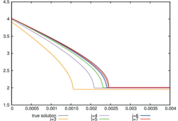
Figure 4: (PFEM) Comparison of the energiesF andFh for the benchmark problem 1 withT=4×10⁻³. The uniform time step size is chosen asτ=10−5, while the spatial discretizations are proportional to2−j,j=3,···,7.
Very similar energy plots can be obtained for the other variants of PFqua-FEM and those of PFobs-FEM. We note that for decreasingε, the time step sizeτneeds to be chosen smaller and smaller in order to capture the correct time scaling of the evolution. We compare this computation for PFqua(i) -FEM, which uses a semi-implicit discretization in time, now with one computation for the implicit time discretization as in (3.20). Here we recall that better accuracy for such discretizations has been reported in [21] for the isotropic Cahn- Hilliard equation, i.e. (3.5a), (3.6a) for (2.2) with (3.4), (3.8)(i) and withϑ=ρ=0. In fact, here we observe a similar behaviour. See Fig. 3, where even for very large choices ofτ the time evolution of the phase field model seems to be captured accurately. Finally, we show some discrete energiesFh≈ F from the parametric scheme PFEM in Fig. 4. Here we choose rather crude discretization parameters, since otherwise the discrete energies Fhwould lie virtually on top of the true energyF.
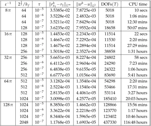
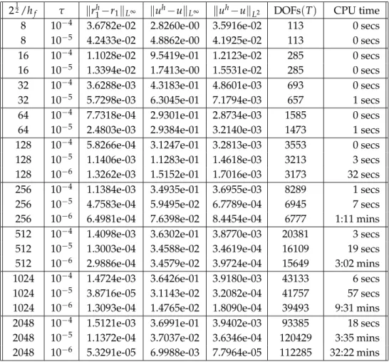
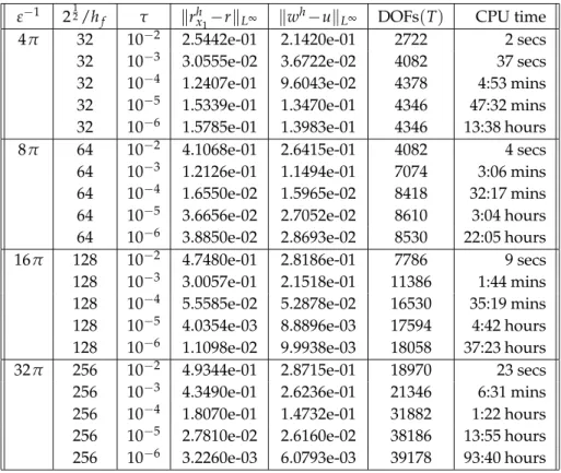
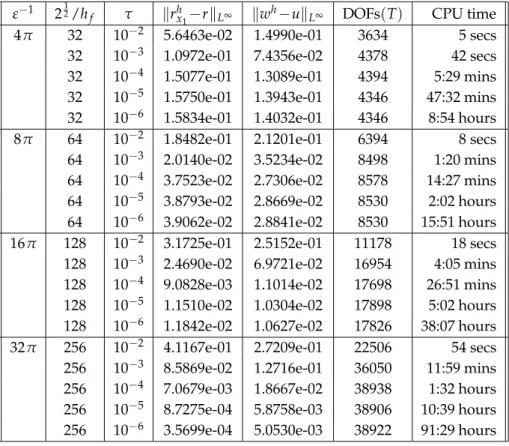
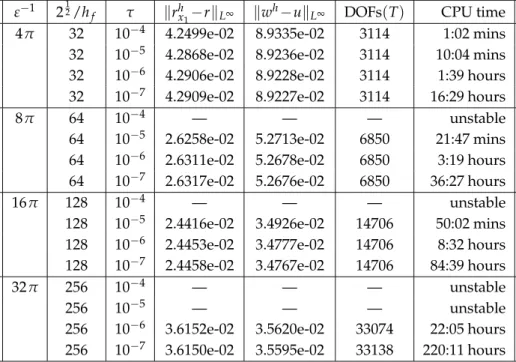
In Table 1 we present the errors in r1 and in u for the scheme PFobs(i)-FEM for a se- lection of interface parametersε and for a range of discretization parameters hf andτ for the benchmark problem 1. The displayed error quantities are defined askwh−ukL2:= (τ∑0≤n≤T/τkwh(·,nτ)−u(·,nτ)k2L2(Ω))12 andkrhx1−r1kL∞:=max0≤n≤T/τ|rhx1(nτ)−r1(nτ)|, whererhx1(t):=inf{s≥0 :ϕh(se1,t) =0}, with e1= (1,0)T being the first unit vector inR2, denotes the phase field approximation of the inner radius. We also show the number of degrees of freedom (DOFs) for the calculation of the discrete solution for the final time step at timet=T. The presented overall CPU times are for a single-thread computation on an Intel i7-860 (2.8 GHz) processor with 8 GB of main memory. For the benchmark problem 1 the remaining variants of PFobs-FEM and PFqua-FEM exhibit very similar er- rors to the ones in Table 1, and so we do not present them here. In later computations we will also employ the stronger normkwh−ukL∞:=max0≤n≤T/τkwh(·,nτ)−u(·,nτ)kL∞(Ω)
for the temperature error. However, for the experiments in Table 1 no convergence can be observed in theL∞(ΩT)-error for the true temperature (4.3) for the phase field approxi- mations. In fact, for the computations in Table 1 the errorskwh−ukL∞ are in the interval