⬎ 0.96) block co- polymers, which favor the bilayered and inter- digitated morphologies (6). This similarity to A7-ZnS structure (f

over many micrometers. Inorganic ZnS nano- crystals were confined at junction areas where two adjacent lamellar layers met. Fluorescent imaging of the film (Fig. 4C) exhibited a pat- tern of ⬃ 1 ␮ m fluorescent lines, corresponding to the ZnS nanocrystals arranged in the film. In a control viral film, without ZnS crystals, no fluorescence was observed (18). Because freely suspended liquid crystalline films form highly ordered structures on the free surface as a result of surface forces (25), smectic O herringbone patterns on the film surface might have higher order than the smectic A or smectic C within inner areas in this film. The observed smectic O morphology of the A7-ZnS film is similar to the high-ratio rod-coil (f

⬎ 0.96) block co- polymers, which favor the bilayered and inter- digitated morphologies (6). This similarity to A7-ZnS structure (f

⫽ ⬃ 0.98) strongly suggests that the A7-ZnS might have interdigitated morphology, where the director (bacteriophage axis) flips by 180° between ad- jacent A7-ZnS particles in the film. Consider- ing the packing free energy, the interdigitated structure might be the most stable structure for the particles having a larger head (20-nm nano- crystal aggregates) and extremely long rod tail particles (Fig. 3, A and B). A schematic dia- gram of the A7-ZnS film is shown in Fig. 4E.

The mechanism for the formation of self- assembled smectic-like lamellar structure of the A7-ZnS film is still being investigated. The morphologies we observe in the film are similar to the results of earlier experiments and theoret- ical work on rigid and flexible block copolymers (6, 26). The A7 phage recognize and physically bind ZnS nanocrystals, preventing macro phase separation into separate organic and inorganic blocks. As the solvent is gradually removed, the virus particles develop orientational order within the suspension and the smecticlike lamellar structure begins to grow from several nucleation points. The mesomorphic structure in the sus- pension is retained even after the complete evaporation of the solvent and forms the highly ordered self-supporting viral film.

Our approach to aligning nanocrystals in a genetically engineered phage-based liquid crys- tal system has several advantages. Monodis- perse biopolymers of specified lengths (A7 phage) can be easily prepared by molecular cloning techniques. By genetic selection of a peptide recognition moiety, one can easily modulate and align different types of inorganic nanocrystals in 3D layered structures (27). Ad- ditionally, we have found that the viral films can be stored at room temperature for at least 7 months without losing the ability to infect a bacterial host and with little loss of titer. This finding indicates that the fabrication of viral film is a reversible process. Moreover, we be- lieve that the film fabrication may constitute a new process for storage of high-density engi- neered DNA. We anticipate that our approach, using recognition as well as a liquid crystalline

self-ordering system of engineered viruses, may provide new pathways to organize electronic, optical, and magnetic materials.

References and Notes

1. J. P. Mathias, E. E. Simanek, G. M. Whitesides, J. Am.

Chem. Soc. 116, 4326 (1994).

2. X. Duan, J. Wang, C. M. Lieber, Appl. Phys. Lett. 76, 1116 (2000).

3. D. J. Norris, M. G. Bawendi, Phys. Rev. B 53, 16347 (1996).

4. C. E. Fowler, W. Shenton, G. Stubbs, S. Mann, Adv.

Mater. 13, 1266 (2001).

5. S. M. Yu et al., Nature 389, 167 (1997).

6. J. T. Chen, E. L. Thomas, C. K. Ober, G.-P. Mao, Science 273, 343 (1996).

7. T. Douglas, M. Young, Nature 393, 152 (1998).

8. A. P. Alivisatos et al., Nature 381, 56 (1996).

9. C. A. Mirkin, R. L. Letsinger, R. C. Mucic, J. J. Storhoff, Nature 382, 607 (1996).

10. P. V. Braun et al., J. Am. Chem. Soc. 121, 7302 (1999).

11. Z. Dogic, S. Fraden, Phys. Rev. Lett. 78, 2417 (1997).

12.

^{, Langmuir} 16, 7820 (2000).

13. J. Lapointe, D. A. Marvin, Mol. Cryst. Liq. Cryst. 19, 269 (1973).

14. S. A. Issaenko, S. A. Harris, T. C. Lubensky, Phys. Rev.

E 60, 578 (1999).

15. S. R. Whaley, D. S. English, E. L. Hu, P. F. Barbara, A. M.

Belcher, Nature 405, 665 (2000).

16. C. E. Flynn, C. Mao, J. L. Williams, B. A. Korgel, A. M.

Belcher, in preparation.

17. C. Mao, C. E. Flynn, A. M. Belcher, in preparation.

18. Supplementary data are available on Science Online at www.sciencemag.org/cgi/content/full/296/5569/

892/DC1.

19. The highest concentration of A7-ZnS suspension was prepared by adding 20 ␮l of 1 mM ZnCl

and Na

S solutions, respectively, into the ⬃30 mg of phage pellet after centrifugation. Various A7-ZnS suspensions were prepared by diluting the smectic A7-ZnS suspensions.

Their concentrations were measured by ultraviolet ab- sorption spectroscopy at 269 nm. These suspensions were transferred to cover slips and 0.7-mm glass capil- lary tubes and characterized.

20. G. W. Gray, J. W. G. Goodby, Smectic Liquid Crystals (L. Hill, Glasgow, 1984), pp. 23–44.

21. One drop of dilute suspension was applied to a TEM grid, washed with distilled water, and quickly dried.

Some samples were stained with 2% uranyl acetate to observe bacteriophage.

22. Bacteriophage pellets were suspended with 400 ␮l of tris-buffered saline ( TBS, pH 7.5) and 200 ␮l of 1 mM ZnCl

to which 1 mM Na

S was added. After rocking for 24 hours at room temperature, the suspension, which was contained in a 1-ml microcentrifuge tube, was slowly dried in a dessicator for 1 week.

23. A7-ZnS films were observed by SEM. For SEM anal- ysis, the film was fractured, then coated via vacuum deposition with 2 nm of chromium in an argon atmosphere.

24. The film was embedded in epoxy resin (LR white) for 1 day and polymerized by adding 10 ␮l of accelerator (London Resin Co. Ltd.). After curing, the resin was thin-sectioned with a Leica Ultramicrotome; ⬃50-nm sections were floated on distilled water and picked up on blank gold grids.

25. A. A. Sonin, N. Clark, Freely Suspended Liquid Crys- talline Films, (Wiley, New York, 1998), pp. 25–43.

26. N. Semenov, S. V. Vasilenko, Sov. Phys. JETP 63, 70 (1986).

27. Although our liquid crystal systems have only incor- porated ZnS at present, our group has already select- ed phage with specific peptide recognition to, and nucleation control of, many materials including II-VI semiconductor crystal surfaces (CdS, PbS, CdSe, ZnSe) and other magnetic materials. Therefore, liquid crystal systems using these and other materials are possible and currently being investigated.

28. We thank J. Williams for assistance in amplifying the clones, J. Mendenhall for assistance in preparation of samples for TEM, J. Ni for assistance in AFM analysis for the cast film, and D. Margolese and E. Ryan for assistance in manuscript editing. The Core TEM and SEM Facilities were used in the Texas Materials Institute, the Center for Nano- and Molecular Science and Technology, and the Institute for Cellular and Molecular Biology. Supported in part by the Army Research Office (Presidential Early Career Award in Science and Engineering), NSF (Nanoscale Interdisciplinary Research Teams), and the Welch Foundation.

14 November 2001; accepted 20 March 2002

Interpretation of Recent Southern Hemisphere

Climate Change

David W. J. Thompson ¹ * and Susan Solomon ²

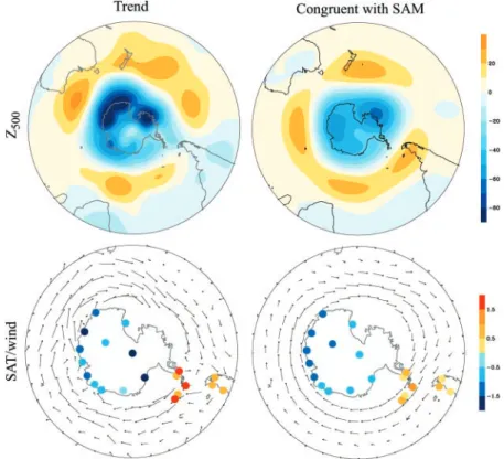
Climate variability in the high-latitude Southern Hemisphere (SH) is dominated by the SH annular mode, a large-scale pattern of variability characterized by fluctuations in the strength of the circumpolar vortex. We present evidence that recent trends in the SH tropospheric circulation can be interpreted as a bias toward the high-index polarity of this pattern, with stronger westerly flow encircling the polar cap. It is argued that the largest and most significant tropospheric trends can be traced to recent trends in the lower stratospheric polar vortex, which are due largely to photochemical ozone losses. During the summer-fall season, the trend toward stronger circumpolar flow has contrib- uted substantially to the observed warming over the Antarctic Peninsula and Patagonia and to the cooling over eastern Antarctica and the Antarctic plateau.

The atmosphere of the SH high latitudes has undergone pronounced changes over the past few decades. Total column ozone losses have exceeded 50% during October throughout the 1990s (1–3), and the Antarctic ozone “hole”

reached record physical size during the spring

of 2000 (4). The lower polar stratosphere has

cooled by ⬃ 10 K during October-November

since 1985 (5, 6), and the seasonal breakdown

of the polar vortex has been remarkably de-

layed: from early November during the 1970s

to late December during the 1990s, in both the

troposphere (7) and the lower stratosphere (1, 7–9). At the surface, the Antarctic Peninsula has warmed by several K over the past several decades, while the interior of the Antarctic con- tinent has exhibited weak cooling (10, 11). Ice shelves have retreated over the peninsula and sea-ice extent has decreased over the Belling- shausen Sea (12–14 ), while sea-ice concentra- tion has increased and the length of the sea-ice season has increased over much of eastern Ant- arctica and the Ross Sea (14–16). Here, we offer evidence that illuminates the connections between these seemingly disparate trends.

We examine climate trends in the high- latitude SH using 30 years (1969 –1998) of monthly mean radiosonde data from seven sta- tions located over Antarctica (Table 1), 32 years (1969 –2000) of monthly surface temper- ature data observations, 30 years (1969 –1998) of ground-based total column ozone measure- ments from Halley station, and 22 years (1979 – 2000) of tropospheric geopotential height data from the National Centers for Environmental Prediction/National Center for Atmospheric Research (NCEP/NCAR) reanalysis (17 ). The

choice of periods used in the analysis was mo- tivated by the facts that (i) the radiosonde and surface temperature records are most complete after ⬃ 1969, (ii) the radiosonde data are only available through 1998, and (iii) the NCEP/

NCAR reanalysis agrees best with the radio- sonde data after ⬃ 1979 (18).

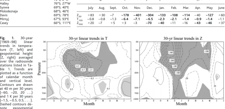
The mean atmospheric circulation of the mid-high latitude SH is dominated by a westerly circumpolar vortex that extends from the surface to the stratosphere. The vortex is strongest dur- ing midwinter in the stratosphere, when polar temperatures are coldest, and is weakest during the summer months, when the circulation at levels above ⬃ 30 hPa reverses sign and be- comes weak easterly. The vortex exhibits con- siderable variability on month-to-month and year-to-year time scales. As shown in Fig. 1, it has also exhibited a pronounced trend over the past few decades. The temperature and strength of the SH polar vortex were estimated by aver- aging temperature and geopotential height anomalies, respectively, over the seven Antarc- tic radiosonde stations listed in Table 1 at levels throughout the depth of the troposphere and stratosphere. Because variability in geopotential height is largest in high latitudes, low geopoten- tial heights over the Antarctic continent are con- sistent with anomalously strong westerly flow along ⬃ 60°S, and vice versa. In the lower polar stratosphere, the trends are dominated by falling geopotential height and cooling that peaks dur- ing the SH spring months but persists through- out the summer. Temperature drops exceeding 6 K per 30 years are evident near 100 hPa from October through December, and geopotential

height decreases in excess of 300 m per 30 years are evident at levels upward of 30 hPa from November through December (Table 2). The summertime stratospheric trends are weaker than their springtime counterparts, but nonethe- less exceed 1 standard deviation (SD) of the respective monthly time series. The data also reveal a secondary peak in the stratospheric geopotential height and temperature decreases during May.

The substantial trends in the lower strato- spheric circulation during the spring months have been documented in previous studies (5–

9). Radiative and observational analyses have demonstrated that these trends are dominated by the development of the Antarctic ozone hole (1, 5, 6, 9, 19), with smaller but important contributions from increases in well-mixed greenhouse gases (20) and stratospheric water vapor (19). The results in Fig. 1 and Table 2 further reveal that similar trends have occurred in the troposphere and that there are important differences in the timing of the stratospheric and tropospheric trends. Whereas the strato- spheric trends peak during November, the most pronounced tropospheric trends occur during the summer months of December-January. Like their stratospheric counterparts, the tropospher- ic trends exhibit “dual maxima,” with peak values occurring during both summer (Decem- ber-January) and fall (April-May) (21).

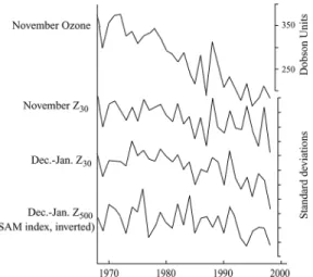
The observed trends in geopotential height over the SH polar regions are consistent with a trend toward the high-index polarity of the SH annular mode (SAM), a large-scale pattern of variability that dominates the SH extratropical

1

Department of Atmospheric Science, Foothills Cam- pus, Colorado State University, Fort Collins, CO 80523, USA.

Aeronomy Laboratory, National Ocean- ic and Atmospheric Administration, 325 South Broad- way, Boulder, CO 80305, USA.

*To whom correspondence should be addressed. E- mail: davet@atmos.colostate.edu

Table 1. Antarctic radiosonde stations used in this study (17).

Station Location

SANAE 70°S; 2°W

Halley 76°S; 27°W

Syowa 69°S; 40°E

Molodeznaja 68°S; 46°E

Davis 69°S; 78°E

Mirnyj 67°S; 93°E

Casey 66°S; 111°E

Fig. 1. 30-year (1969 –98) linear trends in tempera- ture (T, left) and geopotential height (Z, right) averaged over the radiosonde stations listed in Ta- ble 1. Trends are plotted as a function of calendar month and vertical level.

Contours are drawn at 40 m per 30 years (– 60, –20, 20 . . .) and 1 K per 30 years (–1.5, – 0.5, 0.5, . . . ).

Dashed contours de- note geopotential

height and temperature decreases. Shading denotes trends that exceed 1 SD of the respective monthly time series.

Table 2. 30-year (1969–98) linear trends in geopotential height (Z) and temperature (T) averaged over the radiosonde stations listed in Table 1 for levels indicated (meters per 30 years and K per 30 years).

Trends exceeding 1 SD of the respective monthly anomaly time series are in bold type.

July Aug. Sept. Oct. Nov. Dec. Jan. Feb. Mar. Apr. May June

Z

⫹83 ⫹30 –7 –178 –401 –304 –133 –108 –114 –40 –127 ⫹60

T

–0.8 –0.8 –1.3 –6.4 –7.1 –6.5 –2.3 –2.1 –1.4 –0.9 –1.4 –1.1

Z

⫹20 –7 ⫹5 ⫹3 –3 –70 –40 –11 –16 –43 –46 ⫹37

circulation on week-to-week and month-to- month time scales [(22–27) the SAM is also referred to as the High-Latitude Mode (23) and the Antarctic Oscillation (27)]. Months corre- sponding to the high-index polarity of the SAM are characterized by cold polar temperatures, low geopotential height over the polar cap, and strong circumpolar flow along ⬃ 60°S. Months corresponding to the low-index polarity are marked by anomalies in the opposite sense.

Like its Northern Hemisphere (NH) counterpart (28), the SAM is evident year-round in the troposphere but is coupled to the circulation of the lower stratosphere during seasons when the stratospheric polar vortex is perturbed by waves dispersing upward from the troposphere (27 ).

Theory predicts that this coupling should occur when the lower stratospheric circulation is westerly but less strong than a threshold value (29). In the SH, these conditions are met when the polar vortex is decaying (late spring/early summer) and when it is building (fall). As shown in Fig. 1 and Table 2, it is roughly during these seasons that the trends in the tropospheric circulation are largest.

Time series of geopotential height anoma- lies in the lower polar stratosphere during No- vember (when the stratospheric trends are larg- est) were generated by averaging geopotential height anomalies at 30 hPa over all seven Ant- arctic radiosonde stations. Similarly, time series of lower stratospheric geopotential height and the SAM during December-January (when the tropospheric trends are largest) were found by averaging geopotential height anomalies at 30 and 500 hPa, respectively (30). Consistent with previous studies linking ozone depletion with the observed changes in SH spring circulation (1, 5, 6, 9, 19), November values of polar stratospheric geopotential height are strongly correlated with concomitant values of total col- umn ozone from Halley station (Fig. 2 and Table 3). Variability in the lower stratospheric circulation during November is also strongly related to variability in the lower stratospheric circulation during December-January, a rela- tionship that presumably reflects the thermal

memory of the lower stratosphere and the pho- tochemical memory inherent in the ozone field (1). In turn, variability in the stratospheric cir- culation during December-January is strongly coupled with the SAM in the troposphere (Fig.

2 and Table 3). Hence, the results of Figs. 1 and 2 imply not only that the impact of springtime ozone losses on the circulation of the lower stratosphere extends into the SH summer months but also that it extends to the circulation of the troposphere. That the trends in springtime ozone exceed those in 30-hPa height reflects the facts that the response of temperature to re- duced ozone is highly nonlinear and is also affected by the slow time scale for radiative relaxation. The direct correlation between No- vember stratospheric circulation anomalies and December-January values of the SAM index is weaker than the concomitant link during De- cember-January but nevertheless exceeds the 95% confidence level (31). The significance of this correlation is not sensitive to shared trends in the time series [see also (32)].

Similar coupling is also evident between the SAM and the strength of the lower strato- spheric polar vortex during April-May, when the tropospheric trends exhibit a secondary maximum. The stratospheric trends during this season are not strongly linked with val- ues of total column ozone during the previous spring (33) but are consistent with the onset of winter season cooling, together with de- pleted ozone during April-May (34, 35).

The trend toward the high-index polarity of the SAM is most pronounced during the De- cember-January and April-May seasons but persists throughout the summer months. The fraction of recent SH high-latitude climate trends that are linearly congruent with the SAM were found by regressing monthly mean values of 500-hPa geopotential height, near-surface (925 hPa) winds, and high-latitude surface tem- perature observations onto standardized De- cember-May monthly mean values of the re- analysis-based SAM index (30) and then mul- tiplying the resulting regression coefficients by the trend in the SAM index (Fig. 3, right pan-

els). The fraction of the trends that are linearly congruent with the SAM are relatively insensi- tive to the trends in the time series (32). The high-index polarity of the SAM favors geopo- tential height decreases throughout the polar cap and anomalously strong westerlies over the Southern Ocean. Because the SAM is accom- panied by thermally indirect vertical motions at polar latitudes, its high-index polarity also fa- vors cooling over much of Antarctica (27). An important exception to this cooling is found over the Antarctic Peninsula (27 ), where anom- alously strong westerlies should act to decrease the incidence of cold air outbreaks from the south and lead to increased warm advection from the Southern Ocean. A similar warm patch is observed over the southern tip of South America, but correlations for surface tempera- tures equatorward of Patagonia were not found to be significant (31), underscoring the fact that the SAM principally influences the polar re- gions of the SH.

The signature of the SAM is strongly re- flected in both the pattern and amplitude of recent trends in the SH tropospheric circulation and surface temperatures over the SH high lat- itudes during the summer-fall season (Fig. 3, left panels). Roughly 44 m of the 51-m-per-22- year (1979 –2000) December-May decreases in 500-hPa geopotential height averaged poleward of 65°S, ⬃ 1.0 of the ⬃ 1.1 K per 32 years (1969 –2000) December-May cooling averaged over the stations in eastern Antarctica and the pole, and ⬃ 0.7 of the ⬃ 1.4 K per 32 years (1969 –2000) warming averaged over the tem- perature data in the peninsula region are linear- ly congruent with the recent trend in the SAM index (32). Hence, not only are the marked trends in the tropospheric circulation during the summer-fall season consistent with the recent trend in the SAM, but so is a substantial fraction of the disparate trends in surface temperature anomalies over the Antarctic continent. The link between the SAM and surface temperature trends is consistent with the observed regionally varying trends in Antarctic sea ice (e.g., de- creases in sea ice near the peninsula accompa- nied by increases over eastern Antarctica). That the trend in the SAM accounts for only ⬃ 50%

of the warming over the peninsula attests to the importance of other climate change mecha- nisms over this region.

The observed trend in the SAM toward stronger circumpolar flow is in the same sense as the trends that have dominated the NH ex- tratropical circulation over the past few decades Fig. 2. Time series of total column

ozone at Halley station and geopoten- tial height anomalies averaged over the radiosonde stations listed in Table 1 for levels and seasons indicated. Negative values denote low values of total col- umn ozone and geopotential height over the pole, and vice versa. Total col- umn ozone is given in Dobson units, and geopotential height is given in SD. In November Z

, 1 SD corresponds to roughly 250 m; in December-January Z

, roughly 100 m; and in December- January Z

, roughly 40 m. The Z

index can be viewed as an inverted in- dex of the SAM (30).

Table 3. Correlation statistics for the time series shown in Fig. 2 (31).

Nov. ozone Nov. Z

DJ Z

Nov. Z

0.73

DJ Z

0.74 0.71

DJ Z

0.42 0.46 0.70

(36–38) but display important differences in their seasonality. Whereas the trends in the SH troposphere peak during the summer and fall seasons, the trends in the NH troposphere peak during the midwinter months January-March (38). The occurrence of positive trends in both the SAM and the NH annular mode (NAM) suggests that the trends reflect processes that transcend the high-latitude climate of a partic- ular hemisphere. Presumably, any climate change mechanism that projects onto the me- ridional temperature gradient in the middle- high latitudes may affect the polarity of the

annular modes. Recent trends in tropical sea- surface temperatures have been shown to affect the NAM (39), and it has been hypothesized (but not yet demonstrated) that a similar link may exist for the SAM (7). Several modeling studies run with increasing greenhouse gases have also simulated the recent trend in the NAM (40–42), and at least three simulations run with increasing greenhouse gases and/or stratospheric ozone losses have derived trends in the modeled SAM that are of the same sign as the observations presented in this paper (42–

44 ). The strong correlation between the SH

stratospheric and tropospheric circulations at a time when the SH polar stratosphere is strongly affected by photochemically induced cooling, as revealed in this study, suggests that Antarctic ozone depletion has played an important role in driving secular variability not only in the cli- mate of the high-latitude SH stratosphere but also at the Earth’s surface there.

The memory in the temperature of the stratospheric polar vortex from spring through summer and the coupling between the strato- sphere and troposphere during the late spring/

early summer months suggest that stratospheric anomalies during spring may provide predictive skill for SH tropospheric climate on month-to- month time scales. Similar predictive skill has already been demonstrated in the NH, where large-amplitude anomalies in the strength of the NH wintertime stratospheric polar vortex fre- quently precede similarly signed anomalies in the lower troposphere (45–47). The statistically significant correlation between the strength of the SH stratospheric polar vortex during No- vember and the tropospheric circulation ⬃ 1–2 months later (Table 3) suggests that a similar link may be important for predicting the climate impacts of the SAM, at least as far north as Patagonia. The “downward propagation” of SH circulation anomalies from the stratosphere to the troposphere during the late spring months is, for example, illustrated by the vertical profile of geopotential height anomalies averaged over the polar cap region during the 2001 spring- summer season (Fig. 4), which constitutes an independent sample from that used in the rest of the analyses. Consistent with the results shown in Figs. 1 and 2, the largest negative anomalies in geopotential height originate at levels above

⬃ 50 hPa during middle November and descend into the troposphere in December. Hence, the month of December 2001 was marked by anomalously high values of the SAM index (Fig. 4, bottom). The time lag of several weeks between anomalies in the stratospheric and tro- pospheric circulations is consistent with results calculated for the NH (45, 46 ).

We have presented evidence that recent trends in the SH tropospheric circulation and surface temperatures over the Antarctic con- tinent are consistent with a systematic bias toward the high-index polarity of the SAM.

The work underscores and clarifies the man- ner in which high-latitude SH climate change over the past several decades has been char- acterized not only by changes in hemispheric mean temperature (48) but also by important changes in the high-latitude circulation.

References and Notes

1. A. E. Jones, J. D. Shanklin, Nature 376, 409 (1995).

2. D. J. Hofmann, S. J. Oltmans, J. M. Harris, B. J. Johnson, J. A. Lathrop, J. Geophys. Res. 102, 8931 (1997).

3. World Meteorological Organization, “Scientific as- sessment of ozone depletion: 1998,” Global Ozone Research and Monitoring Project Rep. 44 (1999).

4. J. K. Angell et al., “Southern hemisphere winter sum- mary 2000” [National Oceanic and Atmospheric Ad- Fig. 3. December-May trends (left) and the contribution of the SAM to the trends (right). Top,

22-year (1979–2000) linear trends in 500-hPa geopotential height. Bottom: 32-year (1969–2000) linear trends in surface temperature and 22-year (1979–2000) linear trends in 925-hPa winds.

Shading is drawn at 10 m per 30 years for 500-hPa height and at increments of 0.5 K per 30 years for surface temperature. The longest vector corresponds to ⬃4 m/s.

Fig. 4. (Top) Geopotential height

anomalies (meters) averaged 65°–90°S

during spring 2001 based on data from

the NCEP-NCAR reanalysis. (Bottom)

Standardized values of the SAM index

(not inverted), as defined in (30). In the

bottom panel, vertical tickmarks denote

1 SD of the SAM index.

ministration (NOAA)/Climate Prediction Center (CPC), Washington, DC (2000)]. Updates are available on the Web at www.cpc.ncep.noaa.gov.

5. K. E. Trenberth, J. G. Olson, J. Clim. 2, 1196 (1989).

6. W. J. Randel, F. Wu, J. Clim. 12, 1467 (1999).

7. J. W. Hurrell, H. van Loon, Tellus 46A, 325 (1994).

8. D. W. Waugh, W. J. Randel, S. Pawson, P. A. Newman, E. R. Nash, J. Geophys. Res. 104, 27191 (1999).

9. S. Zhou, M. E. Gelman, A. J. Miller, J. P. McCormack, Geophys. Res. Lett. 27, 1123 (2000).

10. G. J. Marshall, V. Lagun, T. A. Lachlan-Cope. Int. J.

Climatol., in press.

11. D. G. Vaughan, G. J. Marshall, W. M. Connolley, J. C.

King, R. Mulvaney, Science 293, 1777 (2001) and references therein has a summary of recent temper- ature trends over Antarctica.

12. D. G. Vaughan, S. M. Doake, Nature 379, 328 (1996).

13. S. S. Jacobs, J. C. Comiso, J. Clim. 10, 697 (1997).

14. E. Hanna, Weather 54, 71 (1999).

15. S. E. Stammerjohn, R. C. Smith, Clim. Change 37, 617 (1997).

16. C. L. Parkinson, Ann. Glaciol., in press.

17. Monthly mean radiosonde data for the stations listed in Table 1 were obtained from the NCEP with the assist- ance of J. Caron and K. Trenberth at the NCAR. The stations were chosen on the basis of the temporal continuity of their records. For each station, anomalies exceeding 3 SD about the long-term mean were re- moved from the data. Gridded monthly mean surface air–temperature anomalies were obtained from the Cli- mate Research Unit at the University of East Anglia (49). Monthly and daily means of the NCEP/NCAR reanalysis (50) were obtained through the NOAA Cli- mate Diagnostics Center. Halley station ozone data were provided by the British Antarctic Survey.

18. Data for the radiosonde stations listed in Table 1 and gridded monthly mean surface temperature data over Antarctica are available starting from 1958. However, because the temporal coverage of these data improved markedly in the late 1960s, our analysis is restricted to the period after 1969. Results based on the NCEP/NCAR reanalysis were found to be in excellent agreement with those derived from the radiosonde data after ⬃1979, which corresponds to the introduction of satellite data into the reanalysis assimilation scheme. For example, the monthly mean time series of 500-hPa geopotential height averaged over the radiosonde stations listed in Table 1 is correlated with 500-hPa geopotential height anomalies from the reanalysis averaged over the SH polar cap (poleward of 60°S) at a level of r ⫽ 0.89 for the period 1979–1998, and the amplitude and season- ality of trends calculated from these two time series are virtually identical. Results based on the NCEP/NCAR reanalysis were found to diverge from those derived from the radiosonde data before 1979, particularly in the lower stratosphere. For a thorough comparison of the NCEP/NCAR reanalysis and radiosonde data over Antarctica, see (51).

19. Water vapor and well-mixed greenhouse gas trends are estimated to contribute about 25 and 10%, re- spectively, to the observed cooling trends in the lowermost Antarctic stratosphere, with the remain- der due to the massive depletion of ozone [see (52)].

20. D. T. Shindell, D. Rind, P. Lonergan, Nature 392, 589 (1998).

21. The robustness of the seasonality of the trends was assessed by recalculating the trends for odd-num- bered years only. In both the troposphere and strato- sphere, the trends exhibit a seasonality qualitatively identical to that noted in Fig. 1 and Table 2.

22. M. Shiotani, J. Meteorol. Soc. Jpn. 68, 461 (1990).

23. J. W. Kidson, J. Clim. 1, 183 (1988).

24. D. J. Karoly, Tellus 42A, 41 (1990).

25. D. L. Hartmann, F. Lo, J. Atmos. Sci. 55, 1303 (1998).

26. D. Gong, S. Wang, Geophys. Res. Lett. 26, 459 (2000).

27. D. W. J. Thompson, J. M. Wallace, J. Clim. 13, 1000 (2000).

28. The NH counterpart to the SAM is alternatively re- ferred to as the North Atlantic Oscillation (36, 53), the Arctic Oscillation (37), and the NAM (27).

29. J. G. Charney, P. G. Drazin, J. Geophys. Res. 66, 83 (1961).

30. Time series of the SAM are typically based on the difference in geopotential height between polar and middle latitudes. Because radiosonde data are scarce in

the SH middle latitudes, the SAM index used in this study is based solely on polar data. In practice, the time series of the SAM derived from 500-hPa height anoma- lies averaged over the radiosonde stations in Table 1 is highly correlated with an index of the SAM based on empirical orthogonal function analysis of gridded SH geopotential height anomalies, as used in (24, 26, 27).

The 500-hPa time series shown in Fig. 2 is correlated with the corresponding leading principal component time series of SH (20° to 90°S) 500-hPa geopotential height anomalies from the NCEP/NCAR reanalysis at r ⫽ 0.84, based on all calendar months of the year, 1979–1998.

31. The significance of the correlations in Table 3 was estimated from the t statistic, assuming only one degree of freedom for every 2 years. The significance of the linkages in Fig. 3 was estimated assuming one degree of freedom for every year (the time series used in Fig. 3 consist of 6 months per year).

32. Because the trend in the SAM accounts for a rela- tively small fraction (9%) of the total month-to- month variance during December-May from 1969–

1998, the fractions of the trends that are linearly congruent with the SAM index in Fig. 3 are not strongly sensitive to shared trends in the time series.

For the shortest period of record considered (Decem- ber-May monthly means from 1979–2000), the total fraction was found to vary by ⬃5% when the indices were detrended before the calculation of the regres- sion coefficients.

33. The correlation between the time series of 500- and 30-hPa height anomalies averaged over the polar cap for the April-May season is r ⫽ 0.62. The correspond- ing correlation between April-May 30-hPa height anomalies and total column ozone at Halley station during the previous November is r ⫽ 0.23.

34. H. K. Roscoe, A. E. Jones, A. M. Lee, Science 278, 93 (1997).

35. H. L. Miller, R. W. Sanders, S. Solomon, J. Geophys.

Res. 104, 18769 (1999).

36. J. W. Hurrell, Science 269, 676 (1995).

37. D. W. J. Thompson, J. M. Wallace, Geophys. Res. Lett.

25, 1297 (1998).

38.

, G. C. Hegerl, J. Clim. 13, 1018 (2000).

39. M. P. Hoerling, J. W. Hurrell, T. Xu, Science 292, 90 (2001).

40. D. T. Shindell, R. L. Miller, G. Schmidt, L. Pandolfo, Nature 399, 452 (1999).

41. D. T. Shindell, G. A. Schmidt, R. L. Miller, D. Rind, J.

Geophys. Res. 106, 7193 (2001).

42. J. C. Fyfe, G. J. Boer, G. M. Flato, Geophys. Res. Lett.

26, 1601 (1999).

43. P. J. Kushner, I. M. Held, T. L. Delworth, J. Clim. 14, 2238 (2001).

44. D. M. H. Sexton, Geophys. Res. Lett. 28, 3697 (2001).

45. M. P. Baldwin, T. J. Dunkerton, J. Geophys. Res. 104, 30937 (1999).

46.

^{, Science} 294, 581 (2001).

47. D. W. J. Thompson, M. P. Baldwin, J. M. Wallace, J.

Climate, in press.

48. Intergovernmental Panel on Climate Change, Climate Change 2001: The Science of Climate Change (Cam- bridge Univ. Press, Cambridge, UK, 2001).

49. P. D. Jones, J. Clim. 7, 1794 (1994).

50. M. E. Kalnay et al., Bull. Am. Meteorol. Soc. 77, 437 (1996).

51. G. J. Marshall, J. Clim. 15, 659 (2002).

52. P. M. de F. Forster, K. P. Shine, Geophys. Res. Lett. 26, 3309 (1999).

53. H. van Loon, J. Rogers, Mon. Weather Rev. 106, 296 (1978).

54. We thank K. E. Trenberth, J. Caron, and W. J. Randel (NCAR) for assistance with the Antarctic radiosonde data; T. Gill (South African Meteorological Service) and G. Bodeker (National Institute for Water and Atmospheric Research) for providing additional sta- tion data; P. D. Jones for providing surface tempera- tures over Antarctica; J. M. Wallace, K. E. Trenberth, M. P. Baldwin, and G. Marshall for helpful comments at various stages of this research; and H. K. Kim and W. Higgins at the NOAA CPC for the inspiration for Fig. 4. D.W.J.T. is supported by the NSF under grant CAREER: ATM-0132190.

21 December 2001; accepted 26 March 2002

Archaefructaceae, a New Basal Angiosperm Family

Ge Sun, ¹ * Qiang Ji, ² David L. Dilcher, ³ * Shaolin Zheng, ⁴ Kevin C. Nixon, ⁵ Xinfu Wang ⁶

Archaefructaceae is proposed as a new basal angiosperm family of herbaceous aquatic plants. This family consists of the fossils Archaefructus liaoningensis and A. sinensis sp. nov. Complete plants from roots to fertile shoots are known.

Their age is a minimum of 124.6 million years from the Yixian Formation, Liaoning, China. They are a sister clade to all angiosperms when their characters are included in a combined three-gene molecular and morphological analysis.

Their reproductive axes lack petals and sepals and bear stamens in pairs below conduplicate carpels.

The fossil record provides information about the evolution of major groups of organisms living on Earth today as well as those that have become extinct. The earliest history of flowering plants is poorly documented. Some of the sparse data from fossils have been accommodated into current phylogenetic models. Current phylogenetic studies (1, 2) and recent paleobotanic finds (3) support the nature of the basal angiosperms (Amborella and Nymphaeales) consistent with combined multiple gene and morphologic analyses (4 – 6). Newly discovered fossils reveal a combi-

nation of unique characters. These fossils consist of new material of Archaefructus li- aoningensis (7) and A. sinensis sp. nov. (8), a new species preserved as nearly whole plants in various stages of reproductive maturity.

The fossils were recovered from the lower

part of the Upper Jurassic/Lower Cretaceous

Yixian Formation (9) in Beipiao and

Lingyuan of western Liaoning, China

(41°12 ⬘ N, 119°22 ⬘ E). The formation is at

least 124.6 million years old (10) and may be

as old as uppermost Upper Jurassic (11). All

aspects of these plants are known, including