DIPLOMARBEIT Dissipative Few-Body Quantum Systems

(1)

Unterschrift Betreuer

DIPLOMARBEIT

Dissipative Few-Body Quantum Systems

Ausgef¨uhrt am

Atominstitut der Technischen Universit¨at Wien in Zusammenarbeit mit dem

Institute of Science and Technology Austria unter der Anleitung von

Assistant Prof. Dr. rer. nat. Mikhail Lemeshko und Assistant Prof. Dr. rer. nat. Peter Rabl

durch

Clemens Jochum, B.Sc.

Schlagergasse 1/3 1090 Wien

Wien, 6. November 2016

(2)

(3)

Abstract

Within the scope of this thesis, we show that a driven-dissipative system with few ultracold atoms can exhibit dissipatively bound states, even if the atom-atom interaction is purely repulsive. This bond arises due to the dipole-dipole interaction, which is restricted to one of the lower electronic energy states, resulting in the distance-dependent coherent population trapping. The quality of this already established method of dissipative binding is improved and the application is extended to higher dimensions and a larger number of atoms. Here, we simulate two- and three-atom systems using an adapted approach to the Monte Carlo wave-function method and analyse the results. Finally, we examine the possibility of finding a setting allowing trimer states but prohibiting dimer states.

In the context of open quantum systems, such a three-body bound states corresponds to the driven-dissipative analogue of a Borromean state. These states can be detected in modern experiments with dipolar and Rydberg-dressed ultracold atomic gases.

(4)

(5)

Kurzfassung

Im Rahmen dieser Diplomarbeit wird gezeigt, dass ein getrieben-dissipatives Sy- stem mit wenigen ultrakalten Atomen zu einem dissipativ gebundenen Zustand führen kann, auch wenn die interatomare Wechselwirkung rein abstoßend ist. Die- se Bindung entsteht aufgrund der Dipol-Dipol Wechselwirkung, die auf einen der elektronischen Grundzustände beschränkt ist. Mittels dieser Beschränkung kann erreicht werden, dass der kohärente Besetzungseinfang von der interatomaren Di- stanz abhängt. Die Güte dieser bereits etablierten dissipativen Bindungsmethode wurde im Laufe dieser Arbeit verbessert und auf eine höhere Anzahl von Ato- men in höherdimensionalen optischen Fallen angewendet. In dieser Arbeit werden Zwei- und Drei-Atom Systeme mittels einer adaptierten Version der Monte Carlo Wave-Function Methode simuliert und die Ergebnisse analysiert. Schließlich wird die Möglichkeit eines Parameterbereichs, in dem Trimere gebildet werden können aber Dimere verhindert werden, diskutiert. Solch ein dreiatomiger Bindungszu- stand entspricht dem getrieben-dissipativen Analogon eines Borromäischen Zu- stands im Kontext offener Quantensysteme. Diese neuartigen Zustände können in modernen Quantenoptik-Experimenten mit dipolaren ultrakalten Quantengasen im Rydbergzustand nachgewiesen werden.

(6)

(7)

Acknowledgments

First, I want to express my sincere gratitude to Professor Mikhail Lemeshko for giving me the opportunity to work under his supervision and in his group at the Institute of Science and Technology Austria. Not only was I provided with an inspiring and productive working environment, but I also gained many insights into the world of academic research. I am thankful for his patience and for his scientific and moral support I continuously received during the many ups and downs of this thesis, which allowed me to finally finish my studies. I wish him success in his future scientific endeavors.

Furthermore, I would also like to thank Professor Peter Rabl for his support, his supervision, and for making this collaboration of the University of Technol- ogy and the Institute of Science and Technology Austria possible while keeping bureaucracy at a minimum.

My gratitude for many hours of pleasant company while working together be- longs to all members of the Lemeshko group at the Institute of Science and Tech- nology Austria, whose friendly and kind atmosphere made me feel immediately welcome.

Additionally, I want to express my special thanks to my colleague Dr. Jan Kaczmarczyk. His experienced advice whenever I got stuck on a programming problem was crucial to the success of this thesis. I wish him all the best in his new role as a father.

Creating this thesis was made possible by using many amazing open source projects, in particular the document preparation system L^ATEX and the plotting library “matplotlib” [1].

I would also like to express my heartfelt appreciation for the company of my friends, with many of whom I have come a long way since starting our physics studies together. Our undertakings, often spurred by our shared interests, never cease to excite me.

Finally, I am sincerely grateful for the support I received by my family and the encouragment to pursue my interests. I am especially thankful for the shelter my parents offered, whenever spirits were low and hunger was high.

(8)

(9)

1. Introduction

”Begin at the beginning“, the King said, very gravely,

”and go on till you come to the end: then stop.“

—Lewis Carroll,Alice in Wonderland [2]

In physics, dissipation usually presents an undesirable obstacle in the experimental realisation of coherent quantum systems, which physicists have to over- come. However, the tremendous progress in designing and controlling quantum setups during the last decades [3] has marked a change of paradigm by shifting the notion of dissipation from an adverse secondary effect to an important tool for the preparation of quantum states. This development gave rise to many novel ideas in form of theoretical proposals for dissipative preparation of quantum states [4–21]. In these proposals the interplay between dissipative and coherent dynamics is exploited in order to guide the system to a desired steady state.

There have already been many succesful experimental advances [22–29], defying the challenging nature of these complex setups.

More recently, dissipative binding mechanisms between atoms have been pre- dicted in a variety of settings [30–33]. In this thesis the method proposed by Weimer and Lemeshko, where pairs of atoms in driven-dissipative open quantum systems can form dissipatively bound metastable states [32, 33], is investigated and improved. Additionally, the method is extended to three atoms in order to examine few-body effects in the dissipative setting. Although few- and many- body effects have been a well researched topic since Isaac Newton [34], even today most physicists still rely on the same approach: they assume additive pairwise interactions between the constituent particles and neglect intrinsic higher-order effects. By doing so, however, they ignore that effective many-particle interactions often play an essential role in the emergence of rich and complex behaviours in a large range of systems [35]. Notable three-body phenomena can be found in diverse systems such as ultracold atoms [36], atomic nuclei [37], colloids [38], and even neutron stars [39]. Condensed matter systems, which constitute a true playground for many-body physics, exhibit fascinating phases such as frac- tional quantum Hall states when three-atom interaction terms are included in the Hamiltonian [40–42]. Some of these novel phases even show promise to further the field of topological quantum computation [43].

In the context of controllable quantum systems, a wide variety of intrinsic few-body phenomena have already been studied [44–46], but one of the most in- triguing manifestations of few-atom physics, the emergence of Borromean states,

(12)

has so far remained a topic of closed systems in an equilibrium setting [47, 48].

These trimer states appear in settings which do not allow any dimer states to form. In classical scenarios such as biology [49] and chemistry [50] they can be observed as Borromean rings [51], while in atomic physics they are known as Efimov states [52] and have been subject to succesful experimental investiga- tion [53–59]. The possibility of finding Borromean states in a dissipative setting using the aforementioned method by Lemeshko and Weimer is treated within the scope of this thesis.

The examined systems and the underlying theory are introduced in the next chapter (Chap. 2), whereas computational and numerical methods used in this thesis are presented in Chap. 3. Two- and three-atom systems are examined seperately in Chap. 4 and Chap. 5, respectively. Parameter regimes, where trimer states can emerge, but dimer states can not form, are investigated in Chap. 6.

The final chapter (Chap. 7) gives a short summary of this thesis and an outlook for further development of this topic. Besides some supplementary results (Ap- pendix C), the appendix contains important quantum optic theory (Appendix A) and reference data on caesium (Appendix B).

(13)

2. Model

In One Dimension, did not a moving Point produce a Line with two terminal points?

In Two Dimensions, did not a moving Line produce a Square with four terminal points?

—Edwin A. Abbott, Flatland [60]

In the scope of this thesis, several setups are examined and simulated. These setups vary in the number of their dimensions and in the number of the involved atoms. While initially a one-dimensional two-atomic system is used as a toy model, this system is extended to a two-dimensional two-atomic system, before finally a two-dimensional three-atomic system is investigated. In Sec. 2.1 the different systems are introduced and explained in detail. Furthermore, a thor- ough account of the individual atoms’ electronic energy structure is given. The mechanism giving rise to the dissipative bond is treated in Sec. 2.3. Whereas a description of some of the theoretical aspects, which are crucial for this mechanism, is included in Sec. 2.2 and in Appendix A, the reader is referred to the literature for a more detailed account of the underlying theory [61–65].

2.1. Setup

Trapping Geometry

All systems considered in this thesis consist of two or three identical atoms, which are confined to one- or two-dimensional geometries by optical traps at ultracold temperatures. In order to study few-body phenomena, the densities of the proposed systems have to be such that only few-body processes play a significant role. This is realisable using the current experimental methods [66–

72]. The atom species was chosen to be caesium, whose relevant properties can be seen in Appendix B. The advantage of choosing caesium atoms is their popularity within the experimental few-body physics community [53, 55–59].

The novel dynamics of the proposed systems emerge due to several different effects, which are induced by laser excitation of the atoms. The atoms’ electronic transitions are driven by counterpropagating laser beams resulting in coherent population trapping (CPT), a similar effect to the well-known electromagneti- cally induced transparency (EIT [61]), which is the main mechanism exploited in

(14)

this thesis and which will be explained in detail in Sec. 2.2. Another consequence of this laser irradiation is that the atoms are provided with an electric dipole momentd, if the valence electron is in a certain state. Additionally, a weak electric field aligns the induced electric dipole moments parallel to each other and perpendicular to the trapping plane guaranteeing that the dipole-dipole interaction between two atoms only depends on the set of interatomic distances {r_ij}.

Together, these concurring effects yield the dissipative binding mechanism.

Figure 2.1.: Schematics of the one-dimensional two-atom system: two ultracold atoms (red) are confined by an appropriate one-dimensional optical trap (light blue) while counterpropagating laser beams (green) drive the atoms’ electronic transitions. The atomic interaction is caused by the electric dipole moments (dark blue), which have parallel align- ment due to a weak electric field.

A quasi-one-dimensional system with two atoms, which was used by Lemeshko and Weimer [32, 33], is used as a simple model to explain the interatomic binding mechanism in Sec. 2.3. The setup of this system is shown in Fig. 2.1. Due to the simplicity of this constellation, the interatomic distance r₂₁ =r is sufficient to fully determine the relative configuration of the atoms.

Figure 2.2.: (a) Representation of the two-atom system in two dimensions with interatomic distance r₂₁ = r. (b) Representation of the three-atom system in two dimensions with indicated opening angle Θ and relative distances r₂₁, r₃₁, and r₃₂. The two-dimensional optical trap is indicated in light blue.

(15)

2.1. Setup This model is expanded in Chap. 4, where the motion of the two atoms is now restricted to two dimensions as displayed in Fig. 2.2(a). By orienting the weak electric field, which aligns the dipole moments, perpendicular to the trapping plane, the atoms’ interaction becomes invariant under rotations in the trapping plane. Consequently, only the interatomic distance r21 = r is needed to completely characterise the arrangement of the atoms.

Finally, three identical ultracold atoms confined to a two-dimensional geometry by an optical dipole trap are considered in Chap. 5. This setup is schematically illustrated in Fig. 2.2(b). The relative distances between the three atoms are determined byr₂₁,r₃₁, andr₂₃ or by r₂₁,r₃₁, and Θ. Applying the law of cosines tor₂₁,r₃₁, and Θ yields r₂₃:

r²₂₃=r²₂₁+r²₃₁−2·r₂₁·r₃₁·cos Θ . (2.1)

Electronic Level Structure

A graphical depiction of the level structure of one individual atom is shown in Fig. 2.3. Here, the two ground states, |1i_a and |3i_a, are chosen as two fine or hyperfine components of the ground electronic state. State |2i_a is an electronically excited state. In the examined few-atom systems, which consist of caesium atoms, two different hyperfine components of the 6²S_1/2 state are chosen as states |1i_a and |3i_a, whereas state 6²P_3/2 is chosen as state |2i_a. For detailed information on the cesium D2 line (6²S1/2 →6²P3/2) see Tab. B.2 in Appendix B.

Due to the driving of the transitions, each atom’s electronic energy level structure can be reduced to these three relevant states |1i_a, |2i_a, and |3i_a, which compose a Λ-configuration. Additionally, a highly excited Rydberg state |Ryi_a is coupled to state|1i_a of the Λ-configuration, providing each atom in state|1i_a with the electric dipole moment d pointing perpendicular to the trapping plane in the weak electric field. Coupling to the environment provides the electronically excited state |2i_a with a decay of rate γ, which is assumed to be equal for both decays|2i_a→ |1i_a and|2i_a→ |3i_a. Furthermore, interaction with three external electric fields gives rise to Rabi oscillations with Rabi frequencies Ω₂₁, Ω₂₃, and ΩRy. The concept of Rabi oscillations is explained in detail in Appendix A. It is assumed that the direct transition |3i_a ↔ |1i_a between the ground states is electric dipole forbidden.

(16)

Figure 2.3.: The electronic energy structure of one of the atoms arranged in a Λ-system with all relevant system parameters. The combination of detuning ∆21 and dipole-dipole interaction U⁽ⁿ^a⁾({rij}) yields a distance-dependent detuning ˜∆₂₁({rij}) = ∆₂₁+U⁽ⁿ^a⁾({rij}).

While the two transitions |1i_a ↔ |2i_a and |3i_a ↔ |2i_a are driven with Rabi frequencies Ω₂₁ and Ω₂₃ and detunings ∆₂₁ and ∆₂₃, respectively, state |1i_a is weakly coupled to the Rydberg state |Ryi_a using a two-photon transition in presence of a far-off-resonant field with Rabi frequency Ω_Ry [73–75]. For ∆_Ry >>

Ω_Ry state |Ryi_a can be adiabatically eliminated and an effective dipole moment dis assigned to|1i_a, while states|2i_a and|3i_ado not display any dipole moment.

The strength of this dipole momentd is determined by the dipole moment d₀ of the highly-excited Rydberg state|Ryi_a, ∆_Ry, and Ω_Ry [74]:

d=d₀ Ω_Ry

∆Ry

2

. (2.2)

This dipole moment generates a dipole-dipole interaction U⁽ⁿ^a⁾({r_ij}), wheren_a stands for the number of involved atoms, if more than one atom is in state |1i_a. Consequently the detuning of the transition |1i_a ↔ |2i_a is rendered distance- dependent: ˜∆₂₁({r_ij}) = ∆₂₁+U⁽ⁿ^a⁾({r_ij}).

2.2. Coherent Population Trapping

The phenomenon of CPT, which is caused by the coherent superposition of atomic states, is crucial to the dissipative binding method employed in this thesis. In the following the causes and the effect of CPT are examined [76].

(17)

2.2. Coherent Population Trapping A three-level atom interacting with two fields of frequenciesω₁andω₂ coupling the two lower states to a single excited state, as shown in Fig. 2.4, is considered.

It is assumed that the transition |ai ↔ |bi is electric dipole forbidden. The resulting electronic level structure is called Λ-configuration due to its shape.

Figure 2.4.: Three-level atom in a Λ-configuration interacting with two resonant fields of frequencies ω₁ and ω₂.

In the rotating-wave approximation the system’s Hamiltonian ˆH writes as:

Hˆ = ˆH₀+ ˆH_I ,

and HˆI =−~

2 Ω^∗₁e^iω¹^t|ai hc|+ Ω1e^−iω¹^t|ci ha|

−~

2 Ω^∗₂e^iω²^t|bi hc|+ Ω₂e^−iω²^t|ci hb|

.

(2.3)

Here, the complex Rabi frequencies Ω₁ and Ω₂ are assumed to change slowly in time so that they can be treated as constant. These Rabi frequencies are associated with the coupling of the laser radiation with frequencies ω₁ and ω₂ to the atomic transitions |ai ↔ |ci and |bi ↔ |ci, respectively. The driving of these transitions is assumed to be in resonance (ω₁ =ω_c−ω_a and ω₂ =ω_c−ω_b). See Appendix A for a more detailed explanation of Rabi frequencies.

The state of the three-level atom can be written as|ψ(t)i=α(t)|ai+β(t)|bi+ γ(t)|ci, where α(t), β(t), and γ(t) are complex coefficients. In order to find a steady-state solution of the considered system, we insert|ψ(t)iin the well-known Schr¨odinger equation:

i~

∂

∂t|ψ(t)i= ˆH|ψ(t)i , (2.4)

where the Planck constant is represented by~. Doing so results in the following set of differential equations:

(18)

iα(t) =˙ ω_aα(t)−1

2Ω^∗₁e^iω¹^tγ(t) , iβ(t) =˙ ω_bβ(t)− 1

2Ω^∗₂e^iω²^tγ(t) , iγ(t) =˙ ω_cβ(t)− 1

2Ω₁e^−iω¹^tα(t)− 1

2Ω₂e^−iω²^tβ(t) .

(2.5)

We introduce new complex coefficients in order to rewrite these equations:

A(t) = α(t)eîωâ^t , B(t) = β(t))eîω^b^t ,

Γ(t) = γ(t)e^iω^c^t ,

(2.6)

resulting in the simple set of differential equations seen in Eq. (2.7).

A(t) =˙ iΩ^∗₁ 2 Γ(t) B(t) =˙ iΩ^∗₂

2 Γ(t)

˙Γ(t) = iΩ₁

2 A(t) + iΩ₂ 2 B(t)

(2.7)

We set the time-derivatives of all coefficients to zero ( ˙A(t) = ˙B(t) = ˙Γ(t) = 0) and use the normalisation condition (|α(t)|²+|β(t)|²+|γ(t)|² = 1 and |A(t)|²+

|B(t)|²+|Γ(t)|² = 1) to find the solution to a steady state. The resulting steady- state coefficents are:

A(t) = Ω₂ Ω , B(t) = −Ω₁

Ω , Γ(t) = 0 .

(2.8)

Here the variable Ω stands for p

|Ω₁|²+|Ω₂|². Due to Γ(t) = 0 it is already obvious that the steady-state solution will not contain any population in the excited level |ci. Using Eq. (2.6) and inserting the resulting coefficients into the original state|ψ(t)i, we obtain the steady state:

|ψdark(t)i= Ω2e^−iω^b^t

Ω |ai − Ω1e^−iω^c^t

Ω |bi , (2.9)

(19)

2.3. Dissipative Binding Mechanism where the global phase has been neglected without loss of generality. Because the lack of population in the excited state |ci renders emission and absorption of photons impossible, state|ψ_dark(t)i is called a dark state. The explanation for this phenomenon of coherent population trapping in the two lower levels is the destructive quantum interference of transitions |ai ↔ |ci and |bi ↔ |ci. This means that, if the atom is prepared in the initial state:

|ψ_dark(0)i= Ω₂

Ω |ai − Ω₁

Ω |bi , (2.10)

the considered atom does not absorb any photons and becomes transparent to the incident light fields, even though these fields drive the transitions resonantly.

Thus, we have shown that, if an atom is prepared in a certain coherent superposition of states, it is possible to cancel any absorption even in the presence of resonant transitions. Once the atom is in the dark state |ψ_dark(t)i, it remains in that state at all times t.

2.3. Dissipative Binding Mechanism

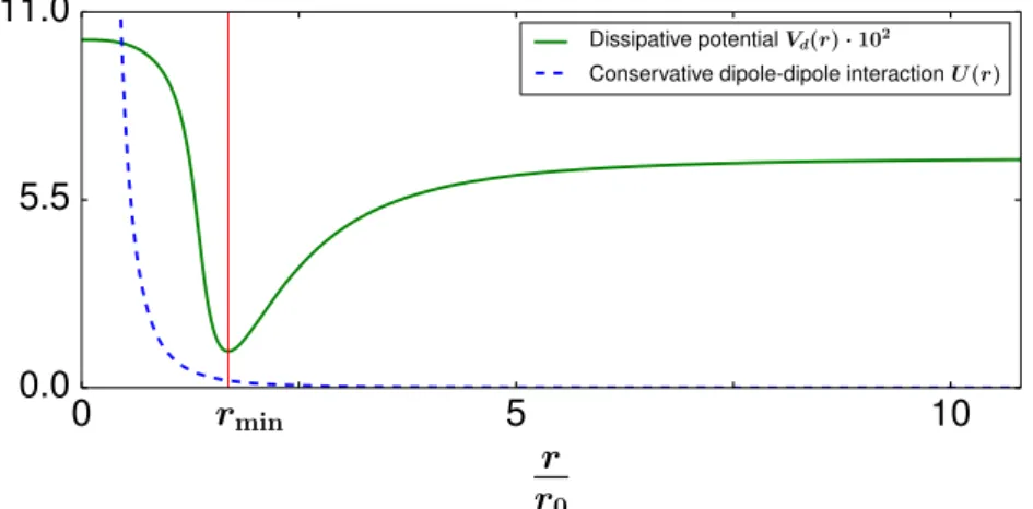
Usually, interatomic binding is caused by conservative interactions acting among electrons and nuclei. The resulting equilibrium configuration is determined by the minimum of the interaction potential. In this section we show that bonding can also occur due to interaction-induced coherent population trapping, which results from non-conservative forces. This dissipatively bound metastable state appears as a stationary state at a preordained interatomic distance. Remarkably, such a dissipatively bound state can arise even when the interactions between the atoms are purely repulsive.

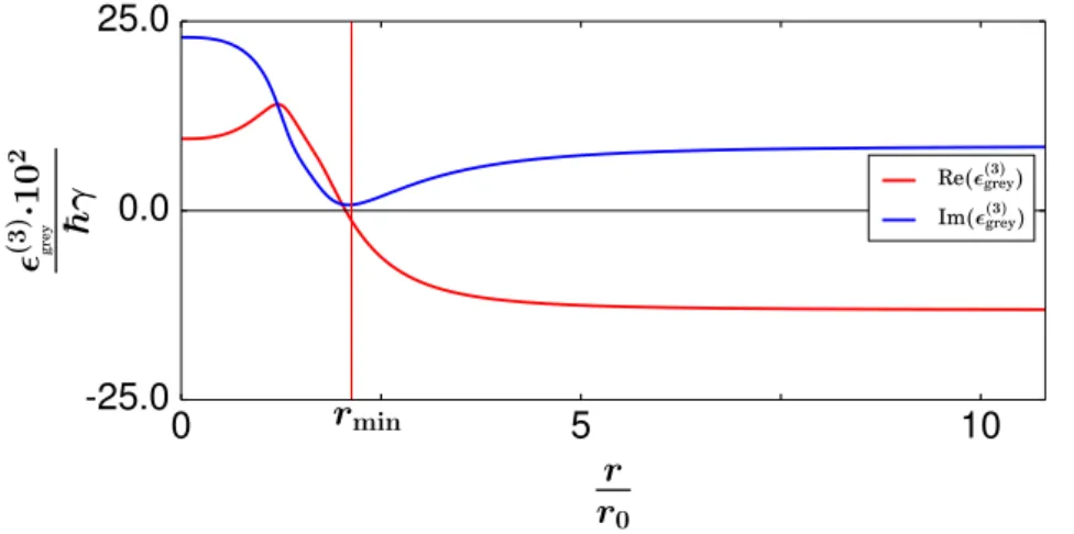
In order to explain the dissipative binding mechanism, we assume a one-dimensional two-atom system, as shown in Fig. 2.1, with the atoms’ electronic energy structure outlined in Fig. 2.3 . We simplify the system by assuming equal Rabi frequencies Ω₂₁ = Ω₂₃ and a resonant transition |3i_a ↔ |2i_a (∆₂₁ = 0). The interaction-induced coherent population trapping, which is the integral aspect of the dissipative binding mechanism, emerges due to the combination of regular CPT in a Λ-system, as described in Sec. 2.2, and the distance-dependent detuning of transition|1i_a↔ |2i_a. The condition for the stationary two-atom state |ψgrey⁽²⁾ i is satisfied at the distance of minimal dissipation r_min. At this distance the two- atom dipole-dipole interaction U⁽²⁾(r₂₁) approximately cancels out the detuning of transition |1i_a↔ |2i_a: U⁽²⁾(r_min) + ∆₂₁≈0.

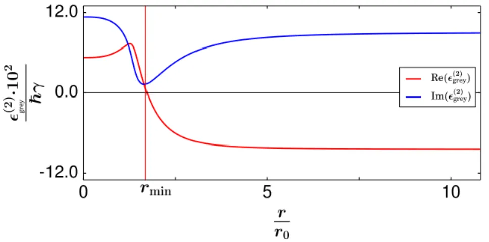
It is noted that due to the restriction of the dipole-dipole interaction to state

|1i_a a true two-atom dark state|ψ_dark⁽²⁾ icorresponding to zero dissipation can not be achieved. Therefore, the obtained state is a so-called grey state|ψ⁽²⁾greyi, where photon absorption is not totally suppressed, but significantly reduced at distance r_min.

(20)

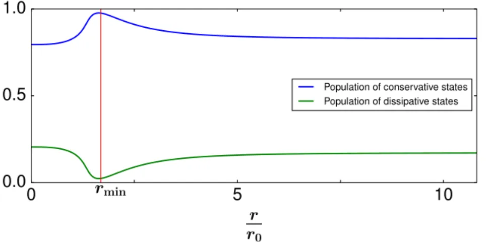
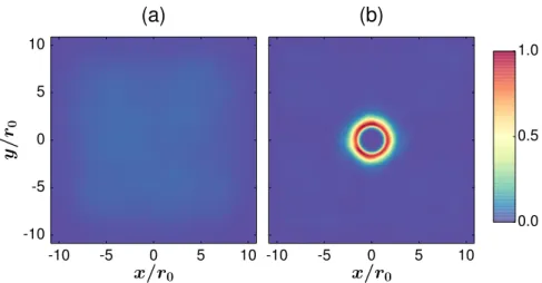
Under this condition the two atoms are almost completely decoupled from photon absorption-emission thereby strongly increasing the probability of finding the atoms separated by distance r_min. In the corpuscular approach, this can be explained by the photon scattering and the corresponding photon recoil due to which the atoms are randomly kicked around until they are in the two-atom grey state|ψgrey⁽²⁾ i, where there is almost no photon scattering. When the dipole- dipole interaction is strong enough to push the atoms apart, they end up in a brighter state, where they experience more photon kicks and are randomly kicked around again until they return to the grey state |ψgrey⁽²⁾ i at distance r_min. This metastable bond is continuously broken and formed by photon scattering and the dipole-dipole interaction. On average, however, there will be a clear peak in the two-body correlation function at distance r_min. When treating the atoms as a wave-function, the leaking of population in the excited state |2i_a due to dissipation is minimised atrmin, resulting in the aforementioned peak of the two- body correlation function. This confinement of the atoms corresponds to the formation of a dissipatively bound state.

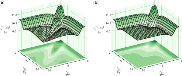
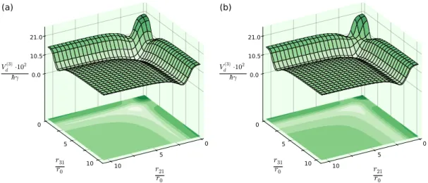
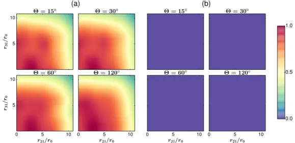
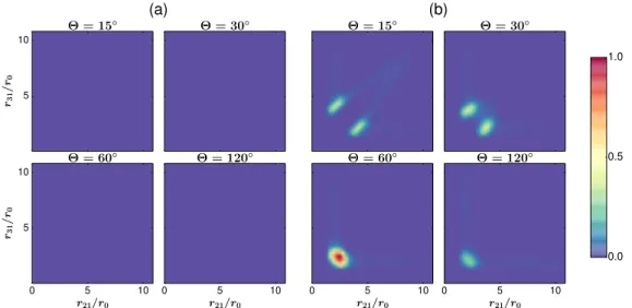
The examined two-dimensional two- and three-atom systems, which have no restrictions on the parameter values, exhibit similar dynamics, but on a more complex level. By setting the parameters Ω₂₁, Ω₂₃, ∆₂₁, ∆₂₃, and d to fixed values the photon absorption rate of our system only depends on the interatomic distances {r_ij}. Different sets of parameter values then yield different distance- dependent behaviours of the photon absorption rate V⁽ⁿ^a⁾({r_ij}), which will be introduced in the next chapter. In Chaps. 4 and 5 we search for shapes of V⁽ⁿ^a⁾({r_ij}) that enhance probability of finding the atoms separated by r_min the most.

(21)

3. Numerical Methods

Physics is mathematical not because we know so much about the physical world, but because we know so little; it is only its mathematical properties that we can discover.

—Bertrand Russell, An Outline of Philosophy[77]

Generally, the time evolution of a quantum system is determined by the initial state of the system and the appropriate quantum master equation, which is a set of differential equations for every element of the system’s density matrix [78].

Due to the complexity and the high computational cost of numerically calculating the time evolution of the systems presented in Sec. 2.1, a more efficient numerical method is necessary. The numerical approach taken in this thesis is based on the Monte Carlo wave-function method (MCWF), which will be treated in Sec. 3.1. In Sec. 3.2 this stochastic method is developed further into an adapted MCWF technique, which was ultimately used to calculate time evolution in this thesis. The novelty of this adapted version is the use of effective dissipative potentials, which will be introduced in Secs. 3.3 and 3.4. The reader is referred to Appendix A and the established literature for more information on the theoretical background of quantum optics [61, 62], statistical physics [78], and quantum mechanics [63–65].

3.1. Monte Carlo Wave-Function Method

Under the assumption of weak coupling between the environment and the system (Born approximation) and the assumption of an environmental correlation time much shorter than the timescale of the system’s evolution (Markov approximation), the time dependence of the system’s reduced density operator ˆρ_S can be calculated by employing the following quantum master equation:

dρˆ_s dt =−i

~

hHˆ_s,ρˆ_si

+L( ˆρ_s) , (3.1)

where~is the reduced Planck constant and ˆρ_sand ˆH_sdenote the reduced density operator and the reduced Hamiltonian, which only account for the dissipative system we want to examine. These operators are derived by tracing over the reservoir variables. By doing so the Lindblad superoperator L( ˆρ_s) is obtained

(22)

simultaneously [79]. This Lindbladian term L( ˆρ_s) is responsible for dissipative processes due to system-environment coupling, while unitary evolution of the system is determined by the system’s Hamiltonian ˆH_s. Equation (3.1) is also known as the Kossakowski-Lindblad equation. A very general form of this Lindblad superoperator L( ˆρs), which is valid for most quantum optics problems involving dissipation, writes as:

L( ˆρ_s) =X

n

γ_n

ˆ

c_nρˆ_scˆ^†_n− 1 2

cˆ^†_ncˆ_n,ρˆ_s

. (3.2)

Here, the operators ˆcn correspond to the jump operators of the system’s decay channels andγ_nare the respective decay rates. In this thesis the jump operators ˆ

c_n represent spontaneous emission of a photon.

Solving this quantum master equation of a system with N states involves cal- culations with the density matrixρ, which contains N ×N terms. For example, the density matrix ρ_s of the system examined in Chap. 5 contains 27×27 = 729 elements only considering the electronic energy structure. In order to describe the time evolution of such a dissipative system more efficiently, the Monte Carlo wave-dunction method (MCWF) developed by K. Mølmer, Y. Castin, and J. Dal- ibard [80, 81] is an excellent candidate. The application of the MCWF method, which is mathematically equivalent to solving the master equation [81], only involves the wave-function, which is described byN instead ofN×N terms. There- fore, the MCWF method is computationally preferable to the density-matrix treatment for any system with a number of states larger than one (N N×N).

Thus, applying the MCWF method is a great way of avoiding costly computation when calculating the time evolution of the systems considered in this thesis.

The integral steps of the MCWF method are applied to a generic system in the following. Assuming an initial state of the system |ψ(t)i at time t, we want to evolve this wave-function in time by a time incrementδt and obtain the final state |ψ⁰(t+δt)i. At first we calculate an intermediary state |ψ⁰(t+δt)i, which is obtained by evolving state|ψ(t)iusing the non-Hermitian Hamiltonian ˆH with quantum jump operators ˆcn [81]:

Hˆ = ˆHs−i~ 2

X

n

γncˆ^†_ncˆn . (3.3) We calculate|ψ⁰(t+δt)iusing the series expansion of the time evolution operator.

By choosing δt sufficiently small, the terms of order O(δt²) and higher can be dropped:

|ψ⁰(t+δt)i= 1− iHδtˆ

~ +O(δt²)

!

|ψ(t)i . (3.4)

(23)

3.1. Monte Carlo Wave-Function Method The second term on the right side of Eq. (3.3) is responsible for the decrease of population in the excited level. In case of the systems introduced in Sec. 2.1 this leads to the reduction of the wave-function wherever the condition for CPT is not satisfied. The square of the time-evolved state|ψ⁰(t+δt)i is given by:

hψ⁰(t+δt)|ψ⁰(t+δt)i=hψ(t)| 1+ iHˆ^†δt

~

!

1− iHδtˆ

~

!

|ψ(t)i . (3.5) The following calulation shows that the wave-function |ψ⁰(t+δt)i is obviously not normalised:

hψ⁰(t+δt)|ψ⁰(t+δt)i= 1− iδt

~ hψ(t)|

Hˆ −Hˆ^†

|ψ(t)i

= 1−δtX

n

hψ(t)|γ_nˆc^†_ncˆ_n|ψ(t)i

= 1−X

n

δp_n= 1−δp with δp_n =δthψ(t)|γ_nˆc^†_nˆc_n|ψ(t)i ≥0 .

(3.6)

A consequence of choosing the size of timestep δt so that this first-order calculation is valid and that the terms of order O(δt²) and higher can be dropped is that hψ⁰(t+δt)|ψ⁰(t+δt)i will be close to one and δp will be small (δp1).

After evolving state |ψ(t)i in time by an increment of δt, the possibility of a quantum jump is examined. Due to the stochastic nature of this step the MCWF method is considered to be part of the Monte Carlo methods. The probability of decay and thus of the wave-function collapsing to a final ground state is given by δp and depends on the amount of population in the excited state. The decision whether a quantum jump happens is done by generating a quasi-random number , which is uniformly distributed between 0 and 1. Then the generated number is compared to δp leading to two cases:

< δp : In this case a quantum jump happens. The new wave-function is then chosen among the different final states:

|ψ(t+δt)i= ˆc_n|ψ(t)i ·(δp_n/δt)⁻¹² . (3.7) The quantum jump associated with operator ˆc_noccurs with a probability of P_n =δp_n/δp. Summing all probabilities P_n yields 1, becauseδp =P

nδp_n.

(24)

> δp: In this case, which will be the majority of the cases since δp1, no quantum jump occurs. The new normalised wave-function at t+δt is calculated by:

|ψ(t+δt)i=|ψ⁰(t+δt)i ·(1−δp)⁻¹² . (3.8) After the stochastic step the obtained normalised wave-function |ψ(t+δt)i becomes the new initial wave-function and the procedure is repeated from the beginning.

The reader is referred to the publication “Monte Carlo wave-function in quantum optics” by K. Mølmer, Y. Castin, and J. Dalibard [81] for a detailed review of the MCWF method, of its equivalence to the master-equation treatment, and of its physical interpretation.

3.2. Adapted MCWF Method

The adapted Monte Carlo method, which will be introduced in this section, was developed in order to simulate the systems in Chaps. 4 and 5. This method is based on the MCWF method discussed in Sec. 3.1. While the MCWF method fully considers the inner electronic energy-level structure of the system, this aspect is integrated out in our approach. This is done by replacing the inner structure with the effective dissipative potential, which will be derived in Secs. 3.3 and 3.4 for two- and three-atom systems, respectively.

Replacing the internal level structure of a n_a-atom system with the effective dissipative potentialV_d⁽ⁿ^a⁾({r_ij}) reduces the size of the Hilbert space by a factor of 3ⁿ^a. Whether the kicks due to photon recoil are accounted for in reference to the center-of-mass frame or in reference to the laboratory frame is unimportant due to the stochastic nature of the photon scattering process. Assuming many photon scattering events the effect on the particle dynamics becomes equivalent in both frames. This enables a further size reduction of the Hilbert space after transforming to relative coordinates.

In the following our adapted MCWF method is applied to the quasi-one-dimensional system with two atoms presented in Sec. 2.1 in order to demonstrate the procedure step by step. The layout of the two-atom system can be seen in Fig. 2.1. Analogous to the MCWF method, our adapted method consists of two steps. First, the wave-function|ψ(t)i is propagated in time by a time increment of δt using the non-Hermitian Hamiltonian ˆH from Eq. 3.3 and replacing the dissipation term by the effective dissipative potentialV_d⁽²⁾({r_ij}):

Hˆ = ˆHkin−i~

2V_d⁽²⁾(r)|ri hr| . (3.9)

(25)

3.2. Adapted MCWF Method Here, the Hamiltonian ˆH_kin = ˆH_s contains the unitary evolution without the inner energy-level structure, i.e., the kinetic energy of the two atoms. Timestep δtis chosen sufficiently small in order to drop terms of order O(δt²) and higher.

The time-evolved state|ψ⁰(t+δt)i, which is not normalised, then writes as:

|ψ⁰(t+δt)i=

1− iδt

~

Hˆ_kin− i~

2V_d⁽²⁾(r)|ri hr|

|ψ(t)i . (3.10) The leaking of population in the excited level is accounted for by the second term on the right hand side in Eq. (3.9). The effect of this term is shown schematically in Fig. 3.1. This step is equivalent to the step in Eq. (3.4). After dropping terms of order O(δt²) and higher, the calculation for the squared norm of the time- evolved state|ψ⁰(t+δt)i can be written as:

hψ⁰(t+δt)|ψ⁰(t+δt)i= 1−δt Z

V_d⁽²⁾(r)| hr|ψ(t)i |²dr = 1−δp (3.11) with δp=δt

Z

V_d⁽²⁾(r)| hr|ψ(t)i |²dr≥0 . (3.12)

r_min r

t=t0

r_min r

t=t0+ ∆t

Dissipative potentialV_d⁽²⁾(r) Wave-functionψ(r, t)

Figure 3.1.: The schematic outline of a two-atom wave-function in relative coordinates ψ(r, t) = hr|ψ(t)i is shown before and after some time

∆t. Due to the distance-dependent population trapping discussed in Secs. 2.3 parts of the wave-function that are close to the dissipative minimumr_min will experience less decay and therefore less leaking of population and less photon scattering than parts further away from r_min. This is accounted for by Eq. (3.9) and accumulates over time, resulting in dissipative binding.

Because the effective dissipative potentialV_d⁽²⁾(r) contains the photon absorption rate depending on the interatomic distance, integrating the wave-function over

(26)

this potential and multiplying the result by the increment δt yields a measure for the probability of decay. The dissipative potential, which corresponds to the dissipation rate at each distance, can not be negative (V_d⁽²⁾(r)≥0).

Analogous to Sec. 3.1, in the second step a pseudo-random numberdistributed uniformly between 0 and 1 is generated and compared toδp:

< δp: In this case, no decay is happening. The majority of the time this case will occur, because ofδp1.

> δp : In this case, decay occurs. A spontaneous photon is emitted.

Because the energy-level structure is integrated out in this approach, the only consequence in this case is a momentum change of the wave-function due to the photon recoil. The emitting atom and the direction of the photon kick are chosen at random. The necessary optical properties of the transition are viewed in Tab. B.2 of Appendix B.

After this step, the wave-function is normalised according to Eq. (3.13) and the procedure is repeated from the beginning.

|ψ(t+δt)i=|ψ⁰(t+δt)i ·(1−δp)⁻¹² (3.13) It is important to note that while the dipole-dipole interactionU⁽ⁿ^a⁾(r) has an effect on the dissipation rate and therefore on the dissipative potential V_d⁽ⁿ^a⁾(r), it also exerts a force on the atoms by shifting the energy of state|1i_a. This effect is not considered in the adapted MCWF algorithm, because it has no significant effect at the observed binding length scales.

The derivations of the dissipative potentials for two- and three-atom systems necessary for this algorithm are shown in the next sections.

3.3. Effective Dissipative Potentials for Two Atoms

After transforming to a suitable rotating frame and applying the rotating wave approximation, the unitary two-atom Hamiltonian ˆH₀⁽²⁾, which does not account for decay, reads as:

Hˆ₀⁽²⁾ = ˆH_kin⁽²⁾+ ˆH_int⁽²⁾ , (3.14)