the few-body spectrum of two interacting bosons in one dimension
Benjamin Geiger,
∗Juan-Diego Urbina, Quirin Hummel, and Klaus Richter Institut f¨ ur Theoretische Physik, Universit¨ at Regensburg, D-93040 Regensburg, Germany
(Dated: May 26, 2017)
We present a semiclassical study of the spectrum of a few-body system consisting of two short- range interacting bosonic particles in one dimension, a particular case of a general class of integrable many-body systems where the energy spectrum is given by the solution of algebraic transcendental equations. By an exact mapping between δ-potentials and boundary conditions on the few-body wavefunctions, we are able to extend previous semiclassical results for single-particle systems with mixed boundary conditions to the two-body problem. The semiclassical approach allows us to derive explicit analytical results for the smooth part of the two-body density of states that are in excellent agreement with numerical calculations. It further enables us to include the effect of bound states in the attractive case. Remarkably, for the particular case of two particles in one dimension, the discrete energy levels obtained through a requantization condition of the smooth density of states are essentially in perfect agreement with the exact ones.
I. INTRODUCTION
The discovery by Bethe of quantum many-body sys- tems admitting analytical expressions for eigenstates and eigenenergies in terms of the implicit solutions of alge- braic transcendental equations [1–3] marked the birth of a whole branch of mathematical physics, namely, the the- ory of quantum integrable models (for an introduction see [4]). Since then, these models have served as the playground to study the role of symmetries and conser- vation laws for the stationary and dynamical properties of many-body systems.
Solvable models had been mainly restricted to the area of mathematical physics because they involve ap- parently unphysical δ-type interparticle interactions and are commonly restricted to one-dimensional (1d) motion.
This situation has drastically changed with the successful preparation of quantum states of interacting cold atoms [5, 6], especially in regimes where the system can be con- sidered essentially 1d, as in elongated optical traps [7–
9]. As it turned out that interactions between neutral cold atoms are described with astonishing precision by δ- type potentials [10–12], the knowledge accumulated dur- ing almost one century of work on solvable models found its way into cold-atom physics during the last decade.
Hence, the experimental study of solvable many-body systems has become a very active field that provides hints for other hitherto unaccessible regimes where external potentials destroy integrability.
There are, however, at least two situations where the detailed level-by-level calculation of the many-body spec- trum using methods of integrable quantum systems over- shoots in the problem of calculating macroscopic proper- ties like the microcanonical partition function. One ex- ample is the thermodynamic limit, where quantum fluc- tuations are suppressed and the spectrum behaves effec-
∗Corresponding author: benjamin.geiger@ur.de
tively smooth. In this regime the appropriate tool is the so-called thermodynamic Bethe ansatz [3]. The second situation appears when studying interacting bosonic sys- tems in the mesoscopic short-wavelength regime, where a separation of scales between the smooth and oscillatory part of the level density allows for the approximation of the spectrum as a smooth function. This is a well known procedure often referred to as Thomas-Fermi approxima- tion [13].
The Thomas-Fermi density of states is of paramount importance as it fixes the energy-dependence of the mean-level spacing, the fundamental energy scale that hallmarks the appearance of quantum effects and deter- mines the relative importance of external perturbations.
In this context, cold atom systems pose an interesting problem: since the Thomas-Fermi approximation explic- itly requires a classical limit for the quantum mechanical Hamiltonian, it is not well defined for systems with δ-like interactions.
All in all, in systems with few particles interacting through short-range interactions, the semiclassical limit appears to be difficult to handle already when we ask for a very fundamental quantity as the mean level spacing.
Our objective in this paper is to show how, by using tech- niques imported from the calculation of Thomas-Fermi approximations in single-particle systems with mixed boundary conditions, one can obtain a rigorous defini- tion of the smooth density of states in systems of few particles interacting through δ-potentials, even when the later do not have a classical limit.
II. ONE PARTICLE IN A DELTA-POTENTIAL In this section we present the general formalism for the calculation of the smooth part of the density of states (DOS) for d-dimensional billiards with either (d − 1)- dimensional δ-barriers (i.e. a δ-function potential along a (d − 1)-dimensional manifold) inside the volume or with Robin (or mixed) boundary conditions on the sur-
arXiv:1705.09637v1 [cond-mat.quant-gas] 26 May 2017
face. The latter case was already discussed by Balian and Bloch [14, 15] and by Sieber [16], but in all three cases the derivations were done via the energy dependent Greens function whereas we use a formalism based on 1d prop- agators [17, 18]. For this we need the propagator for a δ-potential in 1d, which is known exactly from a path integral calculation [19, 20]. Notably, quantum mechan- ical properties, like the appearance of a bound state for attractive interaction, are well hidden inside the results (see e.g. [21]). Therefore we take an alternative approach which is more instructive for our purposes.
A. Propagator for a particle in a delta-potential The 1d-propagator for the δ-barrier is derived in a straightforward way by first calculating the exact propa- gator for a particle on a line with Dirichlet boundary con- ditions at x = ±L and a δ-potential V (x) = ( ~
2κ/m) δ(x) with κ ∈ R and then taking the limit L → ∞. The solu- tions of the stationary Schr¨ odinger equation
− ~
22m
∂
2∂x
2+ ~
2κ m δ(x)
ψ(x) = Eψ(x) (1) for the confined system are well known (see e.g. [22]) and can be separated into symmetric and antisymmetric solutions due to the symmetry of the problem. The latter are not affected by the δ-potential and coincide with the antisymmetric solutions of a particle in a box:
ψ
n(a)(x) = 1
√ L sin(k
n(a)x), k
n(a)= nπ
L , n ∈ N . (2) The symmetric solutions are given by
ψ
(s)n(x) = A
n√
L sin(k
(s)n(|x| − L)), k
(s)nL = nπ − arctan
k
(s)nκ
,
(3)
where A
nis a normalization constant that depends on k
(s)n. The transcendental equation in (3) has exactly one solution for every n ∈ N and another nontrivial solution for n = 0 if κ is negative. In the case κL ∈ (−1, 0) this solution is real whereas the case κL < −1 yields a purely imaginary wave number which corresponds to a negative energy, referred to as a bound state in the following. The two types of states are continuously connected by the zero energy solution
ψ
0(s)(x) = r 3
2L
3(|x| − L) (4) valid for κL = −1. In the limit L → ∞ the state ψ
0(s)will always be bound irrespective of the value of κ.
The exact propagator for the confined system can now be written as
K
bδc(x
0, x, t) =
∞
X
n=1
e
−2mi~t(k(a)n )2ψ
n(a)(x
0)ψ
n(a)(x) +
∞
X
n=0
e
−i~t2m(k(s)n )2ψ
n(s)(x
0)ψ
(s)n(x).
(5)
In the case κ ≥ 0 both summations start with n = 1. In the limit L → ∞ this yields (see App. A)
K
δ(x
0, x, t) = 1 2π
Z
∞−∞
dk e
−2mi~tk2cos(k(x
0− x))
− 1 2π
Z
∞−∞
dk e
−2mi~tk2Re e
ik(|x0|+|x|)1 + i
kκ− Θ(−κ)κe
i~t2mκ2e
κ(|x0|+|x|),
(6)
where the last term originates from the separate treat- ment of the (bound) state ψ
0(s)(Θ is the Heaviside step function). The first integral in (6) can be evaluated di- rectly by means of a Gaussian (or Fresnel) integral and yields the well-known expression for the free propagator
K
0(x
0, x, t) = r m
2πi ~ t e
−2i~tm (x0−x)2. (7) The second integral in (6) can be evaluated in the same way after replacing
1 1 + i
kκ=
Z
∞ 0d e
−(1+ikκ). (8) Finally, the propagator for the Hamiltonian in Eq. (1) reads
K
δ(x
0, x, t) = K
0(x
0, x, t) + K
κ(x
0, x, t), (9) with the deviation from free propagation given by
K
κ(x
0, x, t) = 1 ∓ 1
2 κe
2mi~κ2e
−κ(|x0|+|x|)− κ r m
2πi ~ t Z
∞0
d e
−κe
−2i~tm (|x0|+|x|±)2.
(10)
Here, we identified κ = |κ| and the upper (lower) signs stand for a repulsive (attractive) potential. This result generalizes the propagator found in [23], which is re- stricted to the repulsive case, and is equivalent to the result from path integral approaches [20]. Note that the second term in (10) can be written as
− Z
∞0
d κe
−κK
0(−|x
0|, |x| ± , t), (11)
which is closely related to the correction −K
0(−x
0, x, t)
obtained for a Dirichlet boundary condition (κ → ∞) at
x = 0 [17]. It thus can be interpreted as the propaga-
tion from x to x
0via the δ-potential, taking a detour or
shortcut of length weighted with the density κe
−κ.
B. The DOS for a billiard with a delta-barrier The DOS of a d-dimensional system can be written as the inverse Laplace transform of the trace of the propa- gator [18]:
ρ(E) = L
−1βh Z
d
dx K(x, x, t = −i ~ β) i
(E). (12) Let Ω be the configuration space of a d-dimensional bil- liard with a classically impenetrable thin barrier inside the volume which can be approximated by a δ-potential along a (d − 1)-dimensional smooth manifold. By only taking into account short-time propagation inside the bil- liard we can locally approximate the barrier by (d − 1)- dimensional planes and thus treat the coordinate perpen- dicular to the barrier as independent from the remaining d − 1 tangential coordinates. In this case the local ap- proximation for the propagator can be written as
K
(d)(x
0, x, t) =K
0(d−1)(x
0k, x
k, t)K
δ(x
0⊥, x
⊥, t)
=K
0(d)(x
0, x, t) (13) + K
0(d−1)(x
0k, x
k, t)K
κ(x
0⊥, x
⊥, t).
Here, K
0(d)(x
0, x, t) is the d-dimensional free propagator and x
⊥and x
kare the coordinates perpendicular and tangential to the barrier. The trace is now calculated
assuming that the integration of the perpendicular di- rection converges rapidly and is thus independent of the position at the barrier. By introducing the interaction strength in units of energy,
µ = ~
2κ
22m , (14)
this yields Z
Ω
d
dx K(x, x, t = −i ~ β) = V
Ωm 2π ~
2β
d2+ S
δ2 m
2π ~
2β
d−12× − 1 ± e
µβerfc( p
µβ) + (1 ∓ 1)e
µβ(15)
with the d-dimensional volume V
Ωof the configuration space Ω and the surface S
δof the barrier. The DOS is then given by the inverse Laplace transform of (15). For d = 1 we have to set S
δ= 1 and the DOS is given by
ρ(E) =V
Ωm 2π ~
2 12Θ(E)
√
πE − 1 2 δ(E)
± 1 2π
r µ ˜ E
Θ(E)
E + ˜ µ + 1 ∓ 1
2 δ(E + ˜ µ).
(16)
In all other cases the result is
ρ(E) =V
Ωm 2π ~
2 d2E
d−22Γ(
d2) Θ(E) − S
δ2 m
2π ~
2 d−12E
d−32Γ(
d−12) Θ(E)
± S
δ2 m
2π ~
2 d−12(
L
−1βh 1
β
d−12e
µβerfc( p µβ) i
(E) + (1 ∓ 1) (E + µ)
d−32Γ(
d−12) Θ(E + µ) )
.
(17)
A closed formula for the inverse Laplace transform L
−1βh 1
β
d−12e
µβerfc( p µβ) i
(E) (18)
for arbitrary dimensions d > 1 is given in App. B.
For varying strength of the δ-potential along the sur- face of the barrier, i.e., κ = κ(x), the surface S
δhas to be replaced by the integral operator R
Sδ
d
d−1x . Note that the boundary conditions at the boundary ∂Ω of the billiard are not yet included and the approximation of a flat barrier may fail near the boundary. Furthermore, the above approximation does not include curvature cor- rections.
Now consider a different setup without a δ-barrier in- side the billiard but with Robin- (or mixed) boundary- conditions
∂
∂x
⊥ψ(x)
xs
= κψ(x
s), x
s∈ ∂Ω. (19)
In 1d this is equivalent to a δ-potential ( ~
2κ/m) δ(x
s) at the surface (i.e., the end points of the line segment) while only allowing for solutions symmetric to the endpoints in a coordinate space extended beyond the latter. This means that in the approximation of a locally flat surface of the boundary we only have to replace the propagator K
δin the above derivation by its symmetry-projected equivalent
K
δ+(x
0, x, t) =K
δ(x
0, x, t) + K
δ(−x
0, x, t)
=K
0(x
0, x, t) + K
0(−x
0, x, t) + 2K
κ(x
0, x, t)
(20)
while taking the trace perpendicular to the boundary to one side only. One can easily see that this only adds an additional surface term
S
δ4
m 2π ~
2 d−12E
d−32Γ(
d−12) Θ(E) (21)
to (17), which corresponds to a Neumann boundary con- dition, while the other terms remain unchanged. This is due to the fact that the Robin boundary condition is equivalent to a δ-potential on the surface combined with a Neumann boundary condition in the sense of re- flection symmetry in the extended space. The above re- sult reproduces the first term in the expansion derived in [15]. Note that our approach also comprises the two- dimensional (2d) case, which was treated separately in [15]. This will be essential in the next section, where we will use the results to derive the Weyl expansion for an interacting system.
III. TWO PARTICLES ON A LINE SEGMENT A. Configuration space
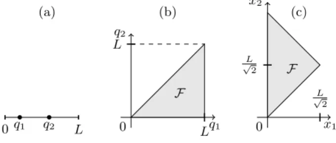
In this section we consider two identical particles on a line with Dirichlet boundary conditions at q = 0 and q = L (two particles in a box, see Fig. 1a). The particles shall interact only when they are at the same point, which is realized by a δ-potential. Furthermore we restrict our- selves to either bosons with zero spin or fermions with spin 1/2. In order to shorten notation, we use imaginary time and choose scaled units, i.e.,
β = it
~
and ~
22m = 1. (22)
Inside the configuration space Ω = {q ∈ R
2| 0 < q
i< L}
the Hamiltonian is given by H(q ˆ
1, q
2) = − ∂
2∂q
12− ∂
2∂q
22+ √
8˜ κ δ(q
1− q
2). (23) After introducing relative and center of mass coordinates
x
1= 1
√
2 (q
1− q
2), x
2= 1
√
2 (q
1+ q
2) (24) the Hamiltonian reads
H(x ˆ
1, x
2) = − ∂
2∂x
21− ∂
2∂x
22+ 2˜ κ δ(x
1). (25) For bosons, the wave functions must be symmetric with respect to particle exchange and, in the case of fermions, an interaction can only occur if the particles have differ- ent spin, i.e., the wave functions must be symmetric, too.
We can therefore restrict ourselves to bosons. For ˜ κ = 0 the system of two indistinguishable particles is equivalent to a system of one quasi-particle of the same mass in the fundamental domain F = {q ∈ Ω | q
1≤ q
2} while requir- ing a Neumann boundary condition on the line q
1= q
2[18]. In the interacting case the same arguments yield the very same equivalence but with a Robin boundary condition
∂
∂x
1ψ(x
1, x
2)
x1=0
= ˜ κψ(0, x
2) (26)
0 q
1q
2L (a)
q
1q
2F L L
0 (b)
x
1x
2F
√L 2
√L 2
0 (c)
FIG. 1. Equivalence of a (a) 1d two-particle system to a (b) 2d one-particle system with fundamental domain F; (c):
fundamental domain after a rotation of the coordinates.
on the symmetry line instead, as illustrated in figure 1(b),(c).
B. Smooth part of the DOS
Using the above equivalence of two particles on a line to one quasi-particle in the fundamental domain we can calculate the DOS directly from (17) and (21):
ρ(E) = L
28π Θ(E) − (2 + √ 2)L 8π
Θ(E) √ E
±
√ 2L 4π
√ Θ(E) E + ˜ µ + θ
10√ 2L 2π
Θ(E + ˜ µ)
√ E + ˜ µ + ρ
c(E),
(27)
with ˜ µ = ˜ κ
2in scaled units (22). We introduced the abbreviation θ
01= (1 ∓ 1)/2 here in order to shorten notation. The last term ρ
c(E) represents the contribu- tions coming from the corners in the fundamental do- main. Here we need the contribution from a π/4 corner with Dirichlet and Robin boundary conditions along the rays. The exact propagator for such a corner can be de- rived from the propagator for a π/2 corner with Robin boundary conditions on the axes,
K
π2
(x
0, x, t) = K
δ+(x
01, x
1, t)K
δ+(x
02, x
2, t). (28) The Dirichlet boundary condition at x
1= x
2can be sat- isfied by antisymmetrizing K
π2
with respect to this line.
This yields the expression K
π4
(x
0, x, t) = 1 2 h
K
π2
((x
01, x
02), (x
1, x
2), t)
− K
π2
((x
02, x
01), (x
1, x
2), t) i .
(29)
The factor 1/2 was chosen such that the trace can be taken in the first quadrant instead of only integrating the inside of the corner. This is possible due to the sym- metry of K
π2
. It is now convenient to write the symmetric propagator (20) as
K
δ+(x
0, x, t) = K
0(x
0, x, t) + K
R(x
0, x, t) (30)
x
1x
2Diric hlet
Diric hlet mixed
mixed
1
2 3
4
5
6 7
8
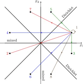
FIG. 2. Interpretation of the different terms in the propagator (32) for x
0= x numbered in order of appearance.
with
K
R(x
0, x, t) = K
0(−x
0, x, t) + 2K
κ(x
0, x, t). (31) Here K
R(x
0, x, t) can be interpreted as the correction to the free propagator representing the propagation from x to the point x
0via the boundary with mixed boundary condition. The propagator K
π4
now takes the form K
π4
(x
0, x, t) = 1 2
K
0(x
01, x
1, t)K
0(x
02, x
2, t) + K
R(x
01, x
1, t)K
R(x
02, x
2, t) + K
0(x
01, x
1, t)K
R(x
02, x
2, t) + K
R(x
01, x
1, t)K
0(x
02, x
2, t)
− K
0(x
02, x
1, t)K
0(x
01, x
2, t)
− K
R(x
02, x
1, t)K
R(x
01, x
2, t)
− K
0(x
02, x
1, t)K
R(x
01, x
2, t)
− K
R(x
02, x
1, t)K
0(x
01, x
2, t) .
(32)
The interpretation of the different terms for x
0= x is shown in Figs. 2 and 3. Tracing the above propaga- tor will lead to different contributions to the DOS. The first term can be identified as a volume term, and the third and fourth can be combined to a surface term cor- responding to mixed boundary conditions. The surface terms for the Dirichlet boundary are given by the fifth and part of the sixth term. All these contributions have to be dropped to get the parts that arise only from the corner:
K
π4
(x
0, x, t) = 1 2
K
R(x
01, x
1, t)K
R(x
02, x
2, t)
− K
R(x
02, x
1, t)K
R(x
01, x
2, t) + K
0(−x
02, x
1, t)K
0(−x
01, x
2, t)
− K
0(x
02, x
1, t)K
R(x
01, x
2, t)
− K
R(x
02, x
1, t)K
0(x
01, x
2, t) .
(33)
x
1x
2Diric hlet
mixed
0
4
3 2
1
x
1x
2Diric hlet
mixed
0
5
6 7 8
FIG. 3. Interpretation of the terms 1-8 in the propagator (32) associated with the corner as multiple reflections. The trajectories in the right figure include a single reflection at the ray with Dirichlet boundary condition, which results in a minus sign in Eq. (32).
The inverse Laplace transform (12) of the trace of this propagator yields the corner contribution. For the first term in (33) the trace can be calculated separately for each coordinate and the inverse Laplace transform can be calculated as a convolution of the density
L
−1βh Z
∞ 0dx K
R(x, x, t) i (E)
= L
−1βh
− 1 4 ± 1
2 e
µβ˜erfc( p
˜
µβ) + θ
01e
µβ˜i
(E)
= − 1
4 δ(E) ± 1 2π
r µ ˜ E
Θ(E)
E + ˜ µ + θ
10δ(E + ˜ µ)
(34)
with itself. The remaining four term of the propagator (33) are traced as a whole because most of the integrals do not have to be evaluated as they cancel mutually af- ter some elementary manipulations. Altogether, the π/4 corner contribution is
ρ
π4
(E) = 5
32 δ(E) + 1 4π
s
˜ µ E + ˜ µ
Θ(E) E + 2˜ µ
∓ 1 8π
r µ ˜ E
Θ(E) E + ˜ µ ∓ 1
4π r 2˜ µ
E Θ(E)
E + 2˜ µ (35)
− θ
10"
1
4 δ(E + ˜ µ) + 1 2π
s
˜ µ E + ˜ µ
Θ(E + ˜ µ) E + 2˜ µ
# .
Note that all the ˜ µ-dependent expressions give multiples of δ(E) in the limit ˜ µ → 0 (Neumann case), as expected.
Combining this result with the contribution from a π/2
Dirichlet-Dirichlet corner (see e.g. [24]) we finally obtain
the entire DOS for the system
ρ(E) = L
28π Θ(E) − (2 + √ 2)L 8π
Θ(E) √ E ±
√ 2L 4π
√ Θ(E) E + ˜ µ + θ
01√ 2L 2π
Θ(E + ˜ µ)
√ E + ˜ µ + 3
8 δ(E) ∓ 1 4π
r µ ˜ E
Θ(E) E + ˜ µ ∓ 1
2π r 2˜ µ
E Θ(E) E + 2˜ µ + 1
2π s
˜ µ E + ˜ µ
Θ(E) E + 2˜ µ
− θ
10"
1
2 δ(E + ˜ µ) + 1 π
s
˜ µ E + ˜ µ
Θ(E + ˜ µ) E + 2˜ µ
# .
(36)
The above result can be represented in a shorter form if we consider positive energies only. Then the cases of an attractive and a repulsive interaction only differ in the overall sign of the ˜ µ-dependent corner corrections:
ρ
+(E) = L
28π − (2 + √ 2)L 8π
√ 1 E +
√ 2L 4π
√ 1 E + ˜ µ
∓
"
1 4π
r µ ˜ E
1 E + ˜ µ + 1
2π r 2˜ µ
E 1 E + 2˜ µ
− 1 2π
s
˜ µ E + ˜ µ
1 E + 2˜ µ
# + 3
8 δ(E).
(37)
Note that the corner corrections are monotonous and nonzero for E > 0 but vanish for E → ∞. This means that the corner corrections are most important for ener- gies near the ground state or, in the case of an attractive interaction, close to E = 0.
In the regime −˜ µ < E < 0 the DOS is conveniently expressed in terms of the excitation energy E
∗= E + ˜ µ:
ρ
−(E
∗) =
√ 2L 2π
Θ(E
∗)
√ E
∗− 1
2 δ(E
∗)− 1 π
r µ ˜ E
∗Θ(E
∗) E
∗+ ˜ µ . (38) The first two terms correspond exactly to the DOS for one particle of mass 2m on a line with Dirichlet boundary conditions at the end points: for very strong interaction the two particles behave as one single particle. The third term represents the interplay of boundary reflections and the interaction. If integrated from −µ to 0 it reduces the level counting function by exactly 1/2 bound state.
C. Comparison with numerical calculations The comparison with the exact quantum mechanical DOS will be done using the level counting function
N (E) = Z
E−∞
dE
0ρ(E
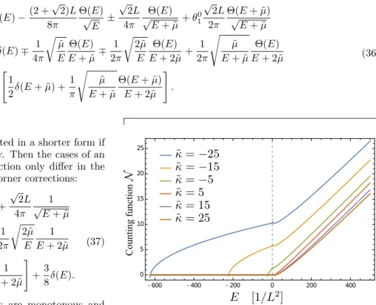
0). (39) In all plots E and ˜ µ will be given in units of 1/L
2(˜ κ in units of 1/L) which is equivalent to setting L = 1 in N . In Fig. 4 the semiclassical level counting function is plotted for −25 ≤ κ ˜ ≤ 25 in steps of ∆˜ κ = 10. For E < 0 the three curves representing the attractive cases κ = −25, −15, −5 resemble 1d single-particle counting functions.
- 600 - 400 - 200 0 200 400
0 5 10 15 20 25
Counting function
FIG. 4. Semiclassical level counting function for L = 1 and values of ˜ κ from -25 (left) to 25 (right) in steps of ∆˜ κ = 10.
x
1x
2m
D D
√L 2
√ 2L
√L 2
0
(a)
x
1x
2m D
D/N
√L 2
√L 2
0
(b)
x
1x
2m
m D D/N
D/N
√L 2
√L 2
0
(c)
FIG. 5. Fundamental domain and equivalent systems. The letters stand for mixed (m), Neumann (N) and Dirichlet (D) boundary conditions.
The exact solutions of the Schr¨ odinger equation for the Hamiltonian (25) can be found by using that the sys- tem is symmetric with respect to the line x
2= L/ √
2.
This means that we can determine a full set of energy
eigenstates that are either symmetric or antisymmetric
to that line [see Fig. 5(a)]. Except for normalization,
this is equivalent to considering only the lower part of
the fundamental domain while requiring either Neumann
or Dirichlet boundary conditions at the symmetry line
[see Fig. 5(b)]. The Dirichlet boundary condition at the
line x
1= x
2corresponds to the antisymmetric solutions
of the extended system shown in Fig. 5(c). Moreover,
the normalization constants for the original and the ex-
tended system are the same. The solutions can be writ-
0 100 200 300 400 500 0
5 10 15
QM SC
Counti ng function
FIG. 6. The quantum mechanical (staircase) and semiclassi- cal level counting functions for ˜ κ = 10 (repulsive case) and L = 1. The functions N
Nand N
Drepresent the limits ˜ κ → 0 and ˜ κ → ∞, respectively.
ten straightforwardly as antisymmetrized products of 1d wave functions.
ψ
Dmn= 1 2
ψ
Dm(x
1)ψ
Dn(x
2) − ψ
mD(x
2)ψ
Dn(x
1) , k
m, k
n∈ Spec
D, 0 ≤ m < n, ψ
Nmn= 1
2
ψ
Nm(x
1)ψ
Nn(x
2) − ψ
Nm(x
2)ψ
Nn(x
1) , k
m, k
n∈ Spec
N, 0 ≤ m < n.
(40)
Here, the 1d wave functions and the sets Spec
N/Dare defined by
ψ
nD(x) = A
Dnsin (k
n(x − d)) , Spec
D=
k
n| k
nd = nπ − arctan k
n˜ κ
, n ∈ N
0∪ n
k
0= i˜ k
0| ˜ k
0= −˜ κ tanh(˜ k
0d), k ˜
0> 0 o , ψ
Nn(x) =A
Nncos (k
n(x − d)) ,
Spec
N=
k
n| k
nd = nπ − π
2 − arctan k
n˜ κ
, n ∈ N
∪ n
k
0= i˜ k
0| ˜ k
0= −˜ κ coth(˜ k
0d), ˜ k
0> 0 o ,
where k
0∈ Spec
Dis chosen either positive or purely imaginary with positive imaginary part depending on the value of κd with d = L/ √
2. The energy eigenvalues of the system are now given as E
mn= k
2m+ k
2nwith k
m, k
neither both in Spec
Dor both in Spec
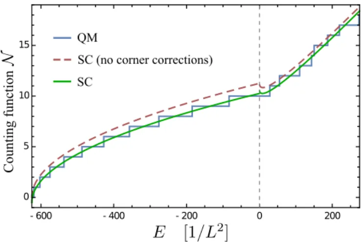
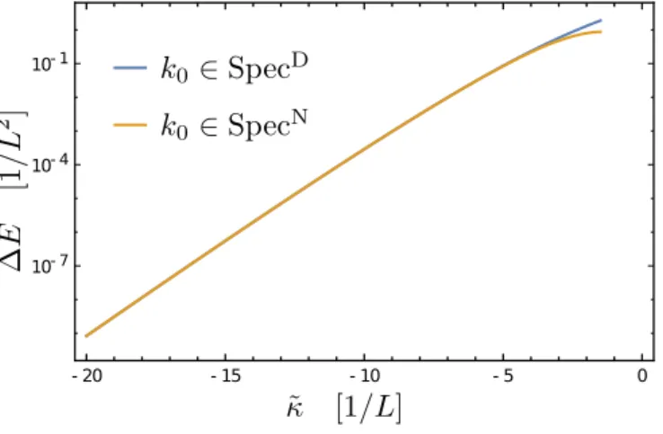
N. The energies have been calculated numerically and the comparison to the smooth level counting function is shown in Fig. 6 for the repulsive case (˜ κ = 10) and in Fig. 7 for the attractive case (˜ κ = −25).
The value ˜ κ = 10 for the repulsive case has been chosen such that the resulting level counting function lies well in between the two limits ˜ κ = 0 and ˜ κ → ∞ corresponding
- 600 - 400 - 200 0 200
0 5 10
15
QM
SC (no corner corrections) SC
Counti ng function
FIG. 7. The quantum mechanical (staircase) and semiclas- sical level counting functions N (E) for ˜ κ = −25 (attractive case).
to non-interacting bosons and fermions (denoted as N
Nand N
Din Fig. 6). For ˜ κ ≥ 0 numerical calculations show that the ratio of corner corrections in the DOS to the full semiclassical DOS at the ground state has a maximum of about 8% for ˜ κ ≈ 5.814 which is very close to the value at which the equation E
0= ˜ κ
2for the ground state energy holds (E
0varies smoothly from E
0= 2π
2for ˜ κ = 0 to E
0= 5π
2for ˜ κ = ∞). As this ratio decreases with the energy the corner corrections can be neglected in the DOS for high energies. This holds also true for the level counting function, where they decrease rapidly from 3/8 to −1/8 as the energy increases.
Figure 7 (attractive case) shows that the corner cor- rections are very important for negative energies and re- sult in a shift by one level in the level counting function at E = 0. In fact the corner corrections give a con- tribution that nearly exactly reproduces the quantum mechanical energy eigenstates. By integrating (38) to get N
−(E
∗) and substituting k
∗= √
E
∗the equation N
−(k
n∗) + 1/2 = n for n ∈ N yields
k
∗nd = nπ
2 − arctan k
∗n˜ κ
(41) which gives exactly the allowed real wave numbers in Spec
Dand Spec
N. Since the negative quantum- mechanical energy levels are always given as E = k
20+k
2nwith k
0purely imaginary and k
nreal we can see that the error in the approximation (41) of the eigenener- gies lies only in the assumption that the imaginary wave numbers k
0in both Spec
Dand Spec
Nare equal to −i˜ κ.
This approximation is very good for large absolute val- ues of ˜ κ and is still reasonable as long as the requanti- zation with ρ
−makes sense, i.e., the ground state en- ergy is negative. The error ∆E = |k
20− ˜ κ
2| of the semi- classically requantized energies is plotted in Fig. 8 for
−20 < ˜ κ < −2. The ground state energy changes sign at ˜ κ = −(3π)/(2 √
2) ≈ −3.332 (semiclassical prediction,
while the quantum mechanical result yields ˜ κ ≈ −3.286).
- 20 - 15 - 10 - 5 0 10- 7
10- 4 10- 1
FIG. 8. The absolute error ∆E
n= |k
02− ˜ κ
2| in the semiclas- sical approximations for k
0in each set Spec
D/N.
At this point the error is less than 0.45/L
2which is small compared to the mean level spacing [ρ
−(˜ µ)]
−1≈ 19/L
2. This shows that the corner corrections are essential for E < 0 and can be used to requantize the system in this regime. Moreover one can use the level counting func- tion directly to find the number of bound states in the system.
IV. CONCLUSION
We presented an alternative derivation for the propa- gator for a δ-potential in Section II A. The resulting ex- pression has a natural interpretation by means of free propagation and hard-wall reflection, taking exponen- tially weighted detours or shortcuts in the cases of repul- sive or attractive interaction, respectively. The propaga- tor can be used to calculate the single-particle DOS for arbitrary shaped billiards of any dimension with mixed boundary conditions and/or δ-barriers inside the volume.
Although the calculations do not include curvature terms the formalism is straightforward and allowed us to calcu- late the corrections from a Dirichlet-Robin (π/4)-corner correction to the DOS which, to our knowledge, have not been calculated before. The corrections given by these corners are, as expected, of lowest order in the energy but give very accurate corrections at low positive ener- gies, where the repulsive and the attractive case differ only in an overall sign. In the attractive case the corner corrections allow for the requantization of the system for negative energies, which shows the accuracy of the ap- proximations used in the formalism.
By using the equivalence of the 1d two-particle prob- lem with δ-interactions to the 2d problem in the funda- mental domain with mixed boundary conditions we pre- sented a powerful tool for the treatment of few-body sys- tems. Its natural application lies in the approximation of the DOS for an arbitrary number of δ-interacting par- ticles. It is important to note that the scattering and
bound states of such a system with infinite volume are known exactly [25]. This means that the short-time prop- agators required for the treatment of higher particle num- bers can, in principle, be calculated directly from them.
Our approach presented here can be extended to include smooth external potentials, which allowed us to examine the thermodynamics of a system of δ-interacting bosons in a harmonic confinement [26].
ACKNOWLEDGMENTS
BG thanks the Studienstiftung des deutschen Volkes for support.
Appendix A: Continuum limit of the propagator The antisymmetric solutions of the confined system have equidistant k’s, i.e. ∆k = k
n+1− k
n= π/L for arbitrary n. So the first line of Eq. (5) is easily verified to have the continuum limit
1 2π
Z
∞−∞
dk e
−2mi~tk2cos(k(x
0− x)) − cos(k(x
0+ x)) ,
whereas the second line needs a more careful treatment.
Omitting the indices we can write 2L
A
2ψ(x
0)ψ(x) = cos(k(|x
0| − |x|))
− cos(k(|x
0| + |x| − 2L)).
Using trigonometric identities and identifying sin(2kL) = 2 tan(kl)
1 + tan
2(kL) = −2
kκ1 +
kκ2cos(2kL) = 1 − tan
2(kL)
1 + tan
2(kL) = 1 −
kκ21 +
kκ2this yields
2L
A
2ψ(x
0)ψ(x) = cos(k(|x
0| + |x|)) + cos(k(|x
0| − |x|))
− 2 Re e
ik(|x0|+|x|)1 + i
kκ,
where the absolute values in the first two arguments can be dropped due to symmetry. Now, observing that A
2= 1 + O(L
−1) and ∆k
n= k
n+1− k
n= π/L +O(L
−2) for all n as L goes to infinity, the continuum limit can be performed exactly in the same way as for the anti- symmetric solutions. The bound state solution of the confined system has an exact limit for the free space, i.e., an exponentially decaying wave function localized at the potential. Summing up all the contributions we get Eq.
(6).
Appendix B: Inverse Laplace transformation
In Eq. (36) we need the inverse Laplace transform f
n(E) of functions of the form
F
n(β) = β
−ne
µβerfc( p
µβ) (B1)
with 2n ∈ N
0. To this end one can use the property of the two-sided Laplace transformation
L
Eh Z
E−∞
dE
0f (E
0) i (β) = 1
β L
Eh f (E) i
(β ) (B2)
to get f
nrecursively from f
0or f
12
. We will take a differ- ent approach that yields the full expression. It is straight- forward to show
nF
n+1(β) =
µ − ∂
∂β
F
n(β) − r µ
π β
−(n+12). (B3)
This can be used to verify by induction the formula F
n(β) = Γ(γ)
Γ(n)
µ − ∂
∂β
n−γF
γ(β)
− r µ
π
n−γ
X
k=1
Γ(n − k) Γ(n)
µ − ∂
∂β
k−1β
−(n−k+12), (B4)
where
γ :=
( 1 n ∈ N ,
1
2
n +
12∈ N . (B5)
Now one can use the linearity of the Laplace transforma- tion and the identity
L
Eh Ef (E) i
(β) = ∂
∂β L
Eh f (E) i
(β) (B6)
to get
f
n(E) = Γ(γ)
Γ(n) (E + µ)
n−γf
γ(E)−
− r µ
π
n−γ
X
k=1
Γ(n − k)
Γ(n)Γ(n − k +
12) (E + µ)
k−1E
n−k−12. (B7)
The functions f
γare given by [27]:
f
γ(E) =
2
π
arctan q
E µ
Θ(E) γ = 1,
√1 π
√Θ(E)
E+µ