Differences by Degree: Evidence of the Net Financial Rates of Return to Undergraduate Study for England and Wales

(1)

Lancaster University Management School Working Paper

2010/038

Differences by Degree: Evidence of the Net Financial Rates of Return to Undergraduate Study for England and Wales

Ian Walker and Yu Zhu

The Department of Economics Lancaster University Management School

Lancaster LA1 4YX UK

provided that full acknowledgement is given.

The LUMS Working Papers series can be accessed at http://www.lums.lancs.ac.uk/publications/

LUMS home page: http://www.lums.lancs.ac.uk/

(2)

Differences by Degree: Evidence of the Net Financial Rates of Return to Undergraduate Study for England and Wales

Ian Walker (LUMS) and Yu Zhu (Kent)

October 2010

Abstract

This paper provides estimates of the impact of higher education qualifications on the earnings of graduates in the UK by subject studied. We use data from the recent UK Labour Force Surveys which provide a sufficiently large sample to consider the effects of the subject studied, class of first degree, and postgraduate qualifications. Ordinary Least Squares estimates show high average returns for women that does not differ by subject.

For men, we find very large returns for Economics, Management and Law but not for other subjects – we even find small negative returns in Arts, Humanities and other Social Sciences. Quantile Regression estimates suggest negative returns for some subjects at the bottom of the distribution, or even at the median. Degree class has large effects in all subjects suggesting the possibility of large returns to effort. Postgraduate study has large effects, independently of first degree class.

A large rise in tuition fees across all subjects has only a modest impact on relative rates of return suggesting that little substitution across subjects would occur. The strong message that comes out of this research is that even a large rise in tuition fees makes little difference to the quality of the investment – those subjects that offer high returns (LEM for men, and all subjects for women) continue to do so. And those subjects that do not (especially OSSAH for men) will continue to offer poor returns. The effect of fee rises is dwarfed by existing cross subject differences in returns

* The data was provided by the UK Data Archive and is used with the permission of the Controller of Her Majesty’s Stationery Office. The data are available on request, subject to registering with the Data Archive. The usual disclaimer applies.

Corresponding author: Professor Ian Walker, Department of Economics, Lancaster University Management School, Lancaster LA1 4YX Email: ian.walker@lancaster.ac.uk

(3)

1. Introduction

This paper provides simple statistical estimates of the correlation between earnings and educational qualifications in England and Wales¹. We adopt regression methods applied to a conventional specification of a model of the determination of earnings². There is a long history of such research in economics, including work that focuses on the impact of academic qualifications – for example, on the impact of an undergraduate degree on earnings, on average: the so-called “college premium”. The literature on the returns to education is well known (see Walker and Zhu (2008)) and reports either the effects of years of schooling or the effects of qualifications. This paper updates the results in Walker and Zhu (2008) with more recent data and exploits information of degree subject and the recent availability of degree class to extend that paper.

The contribution of this paper is fourfold. First, we provide estimates of the college premium, the effect of postgraduate qualifications, and the attainment level of first degree, broken down by the broad subject of the first degree. Secondly, because we wish to make present value calculations and are therefore particularly interested in the lifecycle of earnings, we adopt a simple method that allows our data to identify the effects of experience on earnings separately from cohort effects in wages. Thirdly, we provide Quantile Regression estimates across the distribution of wages. Finally, we use our estimates to make crude comparisons of rates of return to higher education investments by subject and gender under alternative tuition fees.

The existing literature on the effect of “college major” is very thin (see Sloane and O‟Leary (2005) and references therein) but the studies that do exist report large differentials by major of study. No studies, to our knowledge, make any attempt to deal with the complex selection issues associated with major choice. Nor do they allow for the impact of taxation or tuition fees. The literature on the impact of postgraduate qualifications on earnings is similarly thin. A notable exception is Dolton et al (1990) for the UK but this uses a 1980 cohort of UK university graduates with earnings data observed just six years later so that they only identify qualification effects at a single, and early, point in the lifecycle – which we show below is a poor guide to lifecycle effects. There is a literature on the impact of college

1 We drop Scotland and Northern Ireland because of differences in their education systems – although including them makes little difference to our analysis.

2 This is the so-called human capital earnings function that restricts (log) earnings to be a linear function of a set

of characteristics, X, and a quadratic function of age (to proxy for work experience). We include qualifications variables into this model as measures of human capital.

(4)

quality (see Eide et al (1998)) for the US. But the UK studies (Chevalier (2009) and Hussain et al (2009)) are again limited to postal surveys of graduates early in their careers.

The paper aims to inform the debate on higher education funding in the UK. We use the latest and largest available dataset and allow our specification of the effects of qualifications on wages to be as flexible as the data can sustain. The major weakness of the research is that we provide estimates of only correlations, not causal effects of subject of study – the “major”. So far little progress has been made in this direction, so we share our weakness with the existing literature. There is an “ability-bias” argument that suggests that our estimates may be an upper bound to the true effect. However, there is a limited amount of evidence from elsewhere that this weakness may not be very important (see Blundell et al (2005)) – at least in the simpler specifications that have been a feature of the previous literature. A further weakness is that we are not able to control for institutional differences:

the data does not identify the higher education institution that granted the qualifications obtained. Again, this is a weakness that we share with the existing literature although there is a small literature on the effect of attending an elite college in the US (see, for example, Hoxby (2009)). In the UK this is also an important issue because it seems likely that there are important differences in the quality of student entrant by institution. Unfortunately, there is very limited data available on institution – the only systematic data is earnings recorded some six years after graduation but the response rate is poor and, as we will see below, early wages are not a good guide to lifecycle effects.

Section 2 reviews the data used here. Section 3 provides econometric estimates of the effects of the key determinants of wages. Section 4 uses these estimates to simulate crude lifecycles of earnings net of tax and tuition fees to allow us to compute private financial rates of return. Section 5 concludes.

2. Data

Our estimation uses a large sample of graduates (i.e. individuals in the data have successfully completed a first degrees) together with individuals who do not have a degree but who completed high school and attained sufficient qualifications to allow them, in principle, to attend university. We think of the latter group as our controls. The data is drawn from the Labour Forces Surveys – the LFS is the largest survey that UK National Statistics conduct, with slightly less than 1% of the population, and contains extensive information about labour market variables at the individual level. We drop all observations who did not

(5)

achieve high school graduation with the level of qualifications to enter university – i.e. less than 2 A-level qualifications. In the UK, HE entry is rationed by achievement recorded at the end of high school and those without the absolute minimum achievements to attend university are excluded here³. We also drop Scotland and Northern Ireland residents and recent immigrants who were educated outside the UK. We use data pooled from successive Labour Force Surveys from 1994 (although information about class of degree was first collected only from 2005) to 2009 (the latest currently available). The resulting sample size is 81,436. Wage data is derived from earnings and hours of work (converted to January 2006 prices using the RPI). Importantly for this work, LFS is a (albeit short) panel dataset from 1997 onwards. Postgraduate qualifications are categorised as either Masters level, PhD level, PGCE (a one year professional training for those entering teaching), and Other (we believe this will be largely qualifications associated with professional training that results in membership of chartered institutes and degrees such as MBA). Table 1 shows the simple breakdown of by gender and postgraduate qualification and Table 2 shows the corresponding average log wages. Women are twice as likely to have PGCE‟s as men, but less likely to have Master or Doctoral degrees. Overall 29% of graduates in our data have postgraduate qualifications and around half of these are to Masters level. Average hourly wage differentials are pronounced: males (females) with first degrees only earn 20% (31%) more than those with 2+ A-levels only – reflecting the lower gender discrimination in the graduate labour market; males (females) with a Masters degree earn 12 % (17%) more than those with a first degree alone; male (female) PhDs earn 4% (7%) more than Masters; male (female) PGCEs earn 6% less (7% more) than those with first degrees alone.

Table 1 Distribution of Highest Qualifications by Gender, %

Qualification Male Female Total

Doctoral 4.68 2.00 3.41

Master 12.09 9.01 10.63

PGCE 3.80 7.96 5.77

Other PG qualification 2.61 2.98 2.78

First degree 56.31 54.65 55.52

2+ A-Levels 20.51 23.41 21.88

Total 100.00 100.00

3 We would like to be able to test the stability of our estimates to this threshold but this is, unfortunately, all the data will allow us to do.

(6)

Table 2 Mean Log Wages by Highest Qualification and Gender

Qualification Male Female Total

Doctoral 2.915 2.783 2.879

Master 2.873 2.712 2.809

PGCE 2.704 2.615 2.646

Other PG qualification 2.838 2.664 2.75

First degree 2.762 2.543 2.66

2+ A-Level 2.566 2.231 2.396

Total 2.742 2.499 2.627

In the UK it is common for undergraduate students to study only a single subject – although this tendency is becoming less pronounced over time. Undergraduate degrees in the data are categorised into 12 subject areas which we, for reasons of sample size, collapse into four broad subject groups: STEM (Science, Technology, Engineering and Medicine which includes mathematics⁴); LEM (Law, Economics and Management), OSSAH (other social sciences, arts and humanities which includes languages), and COMB (those with degrees that combine more than one subject - but we do not know what these combinations are in our data).

Table 3 shows the simple breakdown of log wage by gender and first degree subject of major. The average college premium for OSSAH majors relative to 2+ A-levels (in Table 2) is 5% (18%) for males (females); while for COMB it is 20% (33%) for males (females);

for STEM it is 25% (38%) for males (females); and for LEM it is 32% (42%) for males (females). Table 3 is for all graduates, but similar differentials are obtained just looking at those with a first degree alone.

In the UK first degrees are classified by rank: first class (9.7% of non-missing degrees), upper second class (44.8%), lower second class (34.2%), third class (5.1%) and pass (6.3%). Table 4 shows the simple breakdown of log wage by gender and class of first degree. The premium for an upper second class degree over a lower second degree or worse is 8% (6%) for males (females), and the premium for a first over an upper second is 4% (6%) for males (females).

4 We have grouped architects and graduate nurses into STEM, although their sample size is small enough for this to make no difference to our broad conclusions.

(7)

Table 3 Mean Log Wages by First Degree Major by Gender: All Graduates

First degree major Male Female Total

STEM 2.814

2.893 2.610 2.769

2.609 2.649 2.412 2.557

2.745 2.801 2.499 2.660 LEM

OSSAH COMB

Table 4 Mean Log Wages by First Degree Class by Gender: All Graduates

First degree class Male Female Total

First class 2.868 2.661 2.766

Upper second 2.830 2.605 2.703

Below upper second 2.750 2.545 2.650

Degree class missing 2.821 2.640 2.732

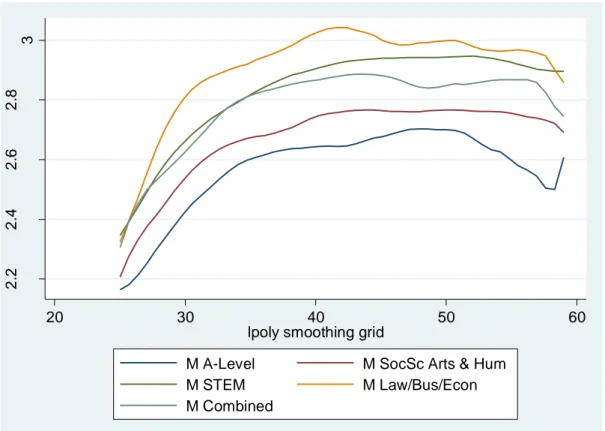
Figures 1 and 2 shows the observed relationship between log wages and age for A- level students and by degree major for men and women respectively. We use local regression methods to smooth the relationship. There are very clear differences between graduates and non-graduates and these differences vary by age for both men and women. There are also differences between majors for graduates which again differ by age. Age-earnings profiles differ and the differences are complicated: they do not appear to be parallel, which is what typical specifications assume. The figure for males suggests that the usual quadratic specification for the age-earnings profile would be a reasonable approximation to the data – but that a single quadratic relationship would be unlikely to fit each major equally well. For example, male LEM students enjoy faster growth in wages early in the lifecycle compared to other majors including STEM. There is no single college premium: wage premia seem to differ by major and by age.

These figures suggest that econometric analysis will need to be sufficiently flexible to capture these differences across majors. Moreover, Figure 2 looks quite different from Figure 1. The age-earnings profiles for women are much flatter - age is a poorer proxy for work experience for women because of time spent outside the labour market. This suggests that the conventional cross-section methods are probably not going to be able to provide a good guide to how the earnings of evolve over the lifecycle women.

(8)

Figure 1 Smoothed Local Regression Estimates of Age – Log Earnings Profiles: Men

Figure 2 Smoothed Local Regression Estimates of Age – Log Earnings Profiles: Women

2.22.42.62.8 3

20 30 40 50 60

lpoly smoothing grid

M A-Level M SocSc Arts & Hum

M STEM M Law/Bus/Econ

M Combined

22.22.42.62.8

20 30 40 50 60

lpoly smoothing grid

W A-Level W SocSc Arts & Hum

W STEM W Law/Bus/Econ

W Combined

(9)

3. Method and Estimates

The conventional approach to estimating the private financial return to education typically uses a simple specification such as:

(1) logw_i   Experience_iExperience_i²δX_iχQ_ie_i for i1..N

where X is a vector of individual characteristics such as migrant status and region of residence, and Q is a vector that records qualifications but, in many studies, simply measures years of completed full-time education. Age is often used as a proxy for work experience.

Here, we focus on graduates, postgraduates and a subset of non-graduates (those that could, in principle, have attended university) and allow differentiation by major studies in Q.

Using a control group that consists of those who might have attended university seems likely to reduce the impact of ability bias on our estimates, and so get us closer to estimating causal effects, although it seems unlikely that it would eliminate it altogether and this needs to be borne in mind when interpreting the estimates.

Our estimates of such the simple specification as (1) reflect the stylised facts that we reported in Section 3 and are not reported here. Rather, since we wish to use our estimates to inform public policy we need to ensure that the specification has the flexibility to reflect the policy issues as well as the realities of the raw data. Section 3 strongly suggests that we should not impose parallel age – earnings profiles so we will provide estimates broken down by highest qualification: that is, separate estimates for those with 2+ A-levels from those with STEM first degree, LEM, etc. That is, we would prefer to estimate

(2) logw_iq   _qExperience_i_qExperience_i²δ X_q _ie_iq for i1.. and N q0..4 which does not impose age earnings profiles to be parallel in q, qualification.

There are two further difficulties. First, as we saw in Section 3, age is a poor proxy for work experience for women. If we wish to model how wages evolve over the lifecycle conditional on continuous participation estimating such a cross section model is not likely to be helpful. The second problem is that it seems likely that there are cohort effects on wages and identifying cohort effects separately from lifecycle effects is impossible with a single cross-section of data and problematic with pooled cross sections over a relatively short span of time. We can resolve both of these difficulties by exploiting the panel element of the data.

If we time difference equation (2) we obtain

(10)

(3) logw_iq _q2_qExperience_iu_iq for i1.. and N q0..4

which allows us to estimate the parameters of the age-earnings profiles, by major (and for the 2+ A-level group) separately from cohort effects providing such cohort effects are additive in equation (2). Indeed, it seems likely that differencing will eliminate some of the unobservable determinants of wage levels that might otherwise contaminate the estimates of the age earnings profile. This then provides independent panel data estimates that can then be imposed in equation (2) which can then be estimated on the pooled cross section data.

Moreover, panel data estimation for employed women provides estimates that are likely to be much closer to the effects of experience. That is, we can then estimate

(4) logw_iq ( )c_i ˆ_qExperience_iˆ_qExperience_i²δ X_q _iv_iq for i1.. and N q0..4 from the pooled cross-section data. Tables 5a (men) and 5b (women) report our baseline OLS pooled cross-section estimates of equation (2) without cohort effects; together with estimates of (3), from the panel, and (4) from the pooled cross sections which include additive cohort effects (we include a cubic in year of birth)⁵. For men, in Table 5a, we find that the estimated lifecycle age-earnings parameters, the γ‟s and β‟s, are reassuringly similar for men whether estimated using the pooled cross-section estimates of the levels equations or from the panel data estimation of the wage difference equations. Nonetheless we find statistically important cohort effects when we impose the lifecycle coefficients from the panel estimation on the pooled cross section estimation of the levels equations. However, for women in Table 5b, we find that the panel estimation provides much steeper age earnings profile estimates – the estimated β‟s are, on average, approximately double those found in the pooled cross section estimates of the levels equation. Moreover, there are larger differences in profiles across majors. Thus, separating the estimation of lifecycle and cohort effects is important, at least for women. The estimates age-experience profiles are plotted in Appendix Figures A1a and A1b - for men the profile for LEM starts higher and is steeper and dominates all other subjects until late in the lifecycle when COMB catches up; for women, LEM and combined are very close but, while other subjects are slightly higher at an early age, their profiles are flatter.

5 We also include controls for region and immigrant status which are not reported but there are no significant

differences in the estimates when we include them. We find that our estimates of the crucial effects are not affected by aggregating the PG qualifications so we group all PG qualifications into a single variable to capture the average effect across all PG qualifications.

(11)

We have included degree class and postgraduate degrees in the specification as simple intercept shifts and we find important differences across subjects. There is a significant premium for degree class that varies across majors: there are particularly large effects for LEM graduates for both men and women; although the differences between first class and upper second class are generally not significant. There is an effect of having PG qualifications over and above the effect of degree class: with large PG premia over and above the first degree effects in all subjects for women and in LEM and COMB for men.

Tables 6a and 6b reports Quantile Regression results for equation (4) (where the estimated experience-earnings profile is drawn from OLS estimates of the wage growth equation using the panel data). Our motivation for investigating the effect of HE across quantiles of the residual wage distribution is the presumption that the latter captures the distribution of unobserved skills. Thus, it is of interest to estimate the effect of HE across this distribution. It is difficult to predict what these effects might look like. On the one hand one might argue that unobserved skills, like perseverance, might complement observed skills (like a specific HE qualification) and that we would therefore expect the Net Present Value (NPV) of a HE qualification to be higher at the top of the distribution than at the bottom. Indeed, low unobserved skills associated with poor high school performance would typically be associated with admission to a low ranked institution that may add less value than a higher rated institution. On the other hand, one might argue that those with poor unobserved skills might attempt to compensate for them by investing (unobserved) greater effort as an undergraduate student. In which case, we might see higher returns at the bottom of the distribution of unobserved skills.

The male premium for a first class is close to 10% across the quartiles for STEM, and the results for women are similar. The upper second premia are also close to 10% for STEM men, but are not significantly different from zero for women. The male LEM first class premia are large for the bottom quartile at 25% and similar for the median, but somewhat smaller for the upper quartile. The LEM bottom quartile female first class premium is very similar to the male premium and are over 30% for the median and top quartile. The LEM upper second premia is slightly smaller than the first premia for men, while for women they are similar to the male premium at the bottom decile but around 15% for the median and top quartile. The upper second effects for COMB men is small across the distribution; and the same is true for women. The first class effect for OSSAH is badly determined for men, while for women there is a 13% effect at the bottom, 9% at the median, but insignificant at the top.

(12)

Table 5a Estimated Age Earnings Profiles by Qualification: Men

Equation (2) Equations (3) and (4)

2+ A‟s STEM LEM COMB OSSAH 2+ A‟s STEM LEM COMB OSSAH

Constant 0.268 (0.257)

0.589 (0.163)

0.111 (0.308)

0.314 (0.278)

0.664 (0.244)

-0.379 (0.022)

-0.217 (0.017)

-1.281 (0.035)

-0.854 (0.029)

-0.554 (0.025)

β 0.109

(0.011)

0.092 (0.007)

0.122 (0.013)

0.116 (0.012)

0.082 (0.010)

0.121 (0.021)

0.107 (0.018)

0.168 (0.031)

0.116 (0.027)

0.130 (0.027)

γ -0.001

(0.000)

-0.001 (0.000)

-0.002 (0.000)

0.001 (0.000)

-0.001 (0.000)

1^st class - 0.075

(0.026)

0.221 (0.065)

0.163 (0.057)

0.052

(0.049) - 0.074

(0.026)

0.224 (0.065)

0.165 (0.058)

0.049 (0.049)

Upper 2^nd - 0.097

(0.018)

0.199 (0.035)

0.049 (0.030)

0.062

(0.026) - 0.095

(0.018)

0.198 (0.035)

0.050 (0.031)

0.061 (0.026) Lower 2^nd

and below - - - -

PG degree - 0.060

(0.018)

0.098 (0.031)

0.119 (0.036)

0.075

(0.027) - 0.048

(0.018)

0.089 (0.031)

0.106 (0.036)

0.051 (0.026) Cohort

effects N N N N N Y Y Y Y Y

R² 0.123 0.175 0.153 0.136 0.137 0.124 0.250 0.188 0.431 0.132

Notes: Region and immigrant controls and missing degree class included. Standard errors in parentheses.

(13)

Table 5b Estimated Age Earnings Profiles by Qualification: Women

Equation (2) Equations (3) and (4)

2+ As STEM LEM COMB OSSAH 2+ As STEM LEM COMB OSSAH

Constant 1.569 (0.220)

1.276 (0.187)

0.794 (0.318)

1.489 (0.227)

1.398 (0.158)

-0.411 (0.019)

0.336 (0.023)

-0.078 (0.042)

-0.242 (0.026)

-0.288 (0.018)

β 0.035

(0.009)

0.059 (0.008)

0.092 (0.014)

0.053 (0.010)

0.049 (0.007)

0.089 (0.020)

0.108 (0.024)

0.125 (0.035)

0.085 (0.024)

0.089 (0.020)

γ -0.000

(0.000)

-0.001 (0.000)

-0.000 (0.000)

-0.001 (0.000)

1^st class - 0.084

(0.033)

0.242 (0.065)

0.054 (0.046)

0.096

(0.033) - 0.082

(0.033)

0.249 (0.065)

0.062 (0.046)

0.100 (0.033)

Upper 2nd - 0.022

(0.022)

0.136 (0.035)

0.064 (0.024)

0.078

(0.018) - 0.021

(0.022)

0.135 (0.035)

0.065 (0.024)

0.078 (0.018) Lower 2^nd

and below - - - -

PG degree - 0.162

(0.020)

0.197 (0.034)

0.164 (0.030)

0.148

(0.018) - 0.153

(0.020)

0.183 (0.034)

0.149 (0.030)

0.123 (0.017) Cohort

effects N N N N N Y Y Y Y Y

R² 0.031 0.103 0.134 0.066 0.106 0.145 0.127 0.184 0.371 0.396

Notes: Region and immigrant controls and missing degree class included. Standard errors in parentheses.

(14)

Table 6a Quantile Regression results: Men

Bottom quartile Median Top quartile

2+ As STEM LEM COMB OSSAH 2+ As STEM LEM COMB OSSAH 2+ As STEM LEM COMB OSSAH

Constant _(0.022)^-0.759 _(0.019)^-0.440 _(0.038)^-1.523 _(0.040)^-1.127 _(0.031)^-0.819 _(0.025)^-0.321 _(0.015)^-0.185 _(0.041)^-1.295 _(0.027)^-0.423 _(0.027)^-0.523 _(0.029)^0.006 _(0.024)^0.050 _(0.044)^-0.924 _(0.030)^-0.242 _(0.030)^-0.242 1^st class ^- _(0.029)^0.098 _(0.074)^0.245 _(0.077)^0.024 _(0.061)^0.001 ^- _(0.022)^0.107 _(0.077)^0.232 _(0.053)^0.178 _(0.051)^0.087 ^- _(0.036)^0.080 _(0.080)^0.162 _(0.061)^0.208 _(0.057)^0.081 Upper 2nd ^- _(0.020)^0.107 _(0.040)^0.180 _(0.041)^0.026 _(0.033)^0.009 ^- _(0.015)^0.105 _(0.042)^0.228 _(0.029)^0.023 _(0.028)^0.089 ^- _(0.025)^0.108 _(0.043)^0.193 _(0.033)^0.059 _(0.031)^0.101 Sub upper

2^nd ^- ^- ^- ^- ^- ^- ^- ^- ^- ^- ^- ^- ^-

PG degree ^- _(0.021)^0.019 _(0.036)^0.094 _(0.049)^0.189 _(0.033)^0.144 ^- _(0.015)^0.023 _(0.037)^0.075 _(0.033)^0.116 _(0.028)^0.067 ^- _(0.024)^0.049 _(0.038)^0.135 _(0.035)^0.094 _(0.031)^0.033

N ¹⁸⁰⁰ ³⁴⁵³ ¹³²² ¹³⁵⁹ ¹⁶⁸² ¹⁸⁰⁰ ³⁴⁵³ ¹³²² ¹³⁵⁹ ¹⁶⁸² ¹⁸⁰⁰ ³⁴⁵³ ¹³²² ¹³⁵⁹ ¹⁶⁸²

Note: Estimates of β and γ are imposed from the right hand blocks of Table 5a. Cohort effects are included throughout. Region and immigrant controls and missing degree class also included. Standard errors in parentheses.

Table 6b Quantile Regression results: Women

Bottom quartile Median Top quartile

2+ As STEM LEM COMB OSSAH 2+ As STEM LEM COMB OSSAH 2+ As STEM LEM COMB OSSAH

Constant _(0.030)^-0.696 _(0.023)^0.336 _(0.049)^-0.423 _(0.034)^0.097 _(0.027)^-0.590 _(0.021)^-0.461 _(0.034)^0.097 _(0.054)^-0.068 _(0.024)^0.399 _(0.019)^-0.234 _(0.028)^-0.105 _(0.026)^0.613 _(0.044)^0.269 _(0.026)^0.613 _(0.018)^0.043 1^st class ^- _(0.033)^0.082 _(0.045)^0.235 _(0.056)^0.016 _(0.047)^0.130 ^- _(0.046)^0.100 _(0.085)^0.330 _(0.066)^0.066 _(0.034)^0.090 ^- _(0.037)^0.055 _(0.070)^0.380 _(0.037)^0.055 _(0.032)^0.035 Upper 2nd ^- _(0.022)^0.021 _(0.042)^0.204 _(0.030)^0.052 _(0.026)^0.129 ^- _(0.031)^0.037 _(0.046)^0.144 _(0.035)^0.057 _(0.019)^0.067 ^- _(0.024)^-0.004 _(0.038)^0.152 _(0.024)^-0.004 _(0.017)^0.022 Sub upper

2^nd ^- ^- ^- ^- ^- ^- ^- ^- ^- ^- ^- ^- ^- ^- ^-

PG degree ^- _(0.020)^0.153 _(0.040)^0.201 _(0.038)^0.191 _(0.026)^0.229 ^- _(0.029)^0.161 _(0.045)^0.169 _(0.043)^0.143 _(0.018)^0.101 ^- _(0.022)^0.157 _(0.037)^0.112 _(0.022)^0.157 _(0.016)^0.067

N ²⁰⁴⁷ ²³¹⁶ ¹¹⁰¹ ¹⁸²⁵ ³¹⁶⁸ ²⁰⁴⁷ ²³¹⁶ ¹¹⁰¹ ¹⁸²⁵ ³¹⁶⁸ ²⁰⁴⁷ ²³¹⁶ ¹¹⁰¹ ¹⁸²⁵ ³¹⁶⁸

Note: Estimates of β and γ are imposed from the right hand blocks of Table 5b. Cohort effects are included throughout. Region and immigrant controls and missing degree class included. Standard errors in parentheses.

(15)

The PG effect is small for STEM men across the quartiles, but around 15% for STEM women across the quartiles. The PG effect for LEM males is 9% for the bottom quartile, slightly lower at the median and slightly higher at the upper quartile; while for women, the effect is 20% at the bottom, lower at the median and about half at the upper quartile. The effect of COMB women is in the mid to upper teen, and somewhat lower for men. The Peffect for OSSAH is 14% for men at the lower quartile, half this at the median, and half again at the upper quartile. A similar pattern holds for OSSAH women but from a higher level.

4. Lifetime impacts and rates of return

The implied college premia will vary with experience, degree class, cohort, and presence of PG qualifications⁶. Thus, in Table 7 we present, using the estimates of equations (3) and (4) from Tables 5a and 5b, the NPVs associated with a lifetime (from 22 to 65) with each major and a lifetime with 2+ A-levels (from 19 to 65) using various discount rates. We also include the internal rate of return (IRR), obtained from grid search. The assumption throughout is that there are tuition fees of either £3,200 or £7,000 pa for three years and opportunity costs are the (discounted) net of tax earnings that they would have received had they not entered university (i.e. those given by the estimates for 2+ A-levels) from 19 to 21.

We allow for income taxes and employee social security contributions using the 2010 schedules⁷. We assume that individuals intend to work full-time throughout their working age lives⁸. We view this as a prospective simulation and focus on a current cohort looking forward. While Table 7 does not allow for the presence of a loan scheme, in Appendix Table A7 we make allowance for this - to the extent that this scheme allows students to shift their tuition costs forward in time with no virtually interest penalty (and that the scheme contains an element of debt forgives) we are underestimating the NPVs (except when the discount rate is zero) and IRRs in Table 7. However, even at a 10% discount rate the differences in NPVs in Table A7 compared to Table 7 are just 3 to 4 thousand pounds.

The IRRs are large for women for all majors and for both good and bad degrees. The tuition fee makes only a small dent in the IRR - around 2 to 2.5%. The differences across majors are very small. For men, there is substantially more variation. The returns to LEM is

6 Surprisingly, we find that the effects of qualifications do not differ across regions. In particular, the impact of major does not vary across regions: which is surprising given the concentration of LEM majors in London.

7 Welfare programmes and the minimum wage are hardly relevant over the range of data being considered here.

8 One might also want to incorporate some part of subsistence costs while studying. For example, many UK students study away from home and incur additional housing costs.

(16)

large for both good and bad degrees, and the tuition fee rise makes a modest difference of around 3%. STEM, Combined and OSSAH all return modest levels according to the calculated IRRs with a bad OSSAH degree generating negative returns – although, in that case, the fee rise has little impact.

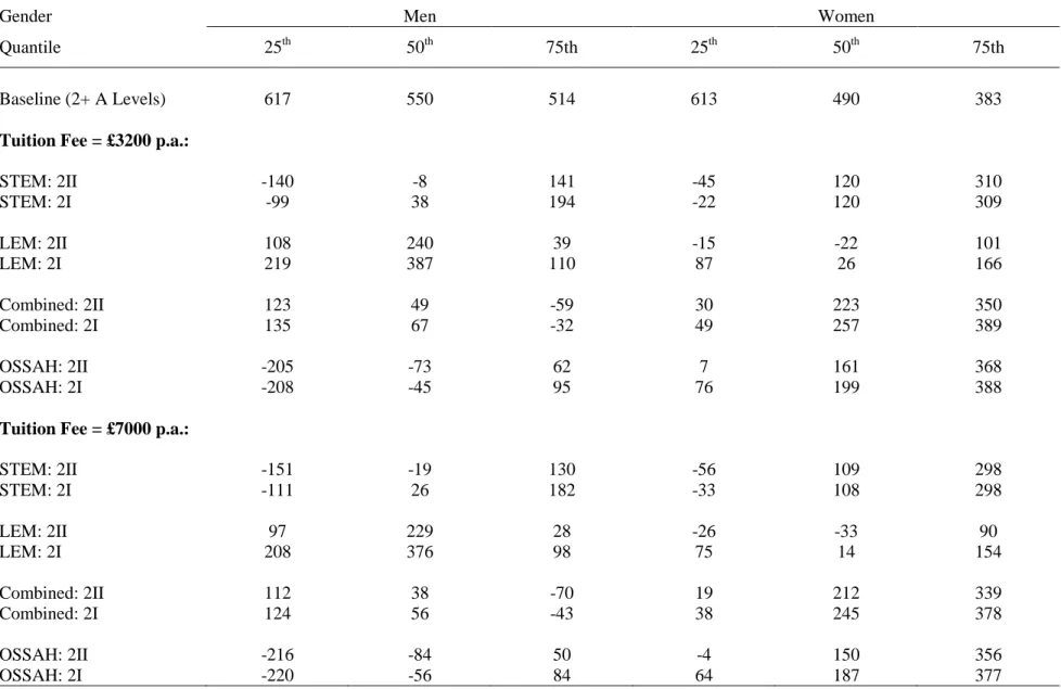
In Table 8 we use the corresponding estimates from tables 6a and 6b to show how the NPV results vary by quantile of the distribution at a given discount rate, 5%, by gender, degree class and major. The median figures in Table 8 are close to the average figures that OLS yields in Table 7. However, there are huge differences across the quantiles within Table 8. Even for women, it would appear that the effects of STEM on NPV at the bottom quartile are much lower and even negative. At higher fees even the STEM median goes negative for women. Huge negative effects are associated with OSSAH for men. Note that the table demonstrates NPVs that rise across the distribution in some cases but not all. For example, for STEM and OSSAH, NPVs rise as we move up the distribution, but the opposite is true for OSSAH. There is no strongly theoretical presumption that any particular pattern should manifest itself and the estimates allow for all possibilities. Table 9 translates the NPV findings across the quantiles into rates of return. This confirms the relatively modest effects of the tuition rise on the returns on student investments. Those subjects that offer low returns at fees of £3200, offer just slightly lower returns at fees of £7000. Subjects that offer high returns at £3200 suffer larger falls if fees rise to £7000, but still offer handsome returns.

5. Conclusion

This paper has used the latest and largest dataset available to estimate as flexible specification as possible. We allowed for tuition fees and the tax system in calculating the NPV associated with higher education (and also the loan scheme). And we provide independent estimates for graduates with different degree majors. The results are large for women - reflecting the greater discrimination that women face in the sub-degree labour market. Indeed, they are large across the board.

The results for men vary considerably across majors: with LEM having very large returns for both good and bad degrees, although higher tuition fees knock around 3% off these figures. The return to STEM is around 5% for a bad degree and 7% for a good one;

COMB degrees are slightly higher; while OSSAH degrees are so low that they turn negative in the case of a bad degree. The first notable feature of the results is that the scale of tuition

(17)

Table 7: NPVs relative to 2+ A-levels (£,000) and IRRs (%)) by Gender, Major, Degree Class, and Discount Rate,

Gender Men Women

Discount Rate 0% 2.5% 5% 7.5% 10% IRR(%) 0% 2.5% 5% 7.5% 10% IRR(%)

Baseline (2+ A Levels) 1679 942 587 403 298 - 1331 766 491 345 262 -

Tuition Fee = £3200 p.a.:

STEM: 2II 226 67 1 -27 -40 5.1 549 290 161 92 51 16.8

STEM: 2I 368 142 46 3 -19 7.7 579 307 172 99 57 17.5

LEM: 2II 1292 671 373 219 133 22.7 700 359 194 108 59 16.8

LEM: 2I 1752 922 523 317 201 28.0 925 484 270 159 95 20.5

Combined: 2II 705 269 92 15 -20 8.3 1080 502 248 127 65 16.3

Combined: 2I 807 322 121 34 -7 9.4 1203 566 285 151 81 17.9

OSSAH: 2II -7 -17 -25 -32 -37 -2.0 1035 469 223 108 49 14.6

OSSAH: 2I 58 20 -3 -17 -26 4.6 1192 551 271 138 71 16.7

STEM: 2II 214 55 -10 -38 -51 4.4 537 278 150 80 40 14.5

STEM: 2I 357 131 35 -9 -31 6.8 567 295 160 88 45 15.1

LEM: 2II 1281 660 362 208 122 20.1 688 347 183 96 48 14.8

LEM: 2I 1741 911 512 305 190 24.8 914 472 259 147 84 18.1

Combined: 2II 694 258 80 4 -31 7.7 1069 491 236 116 53 14.5

Combined: 2I 796 310 110 22 -18 8.6 1191 555 274 140 70 15.9

OSSAH: 2II -18 -28 -37 -44 -49 -2.2 1023 458 212 96 38 13.1

OSSAH: 2I 47 9 -14 -28 -38 3.3 1180 540 259 127 59 14.8

(18)

Table 8: Quantile Regression Estimates of NPVs (graduates are all relative to 2+ A-levels) at 5% Discount Rate, £,000.

Gender Men Women

Quantile 25^th 50^th 75th 25^th 50^th 75th

Baseline (2+ A Levels) 617 550 514 613 490 383

STEM: 2II -140 -8 141 -45 120 310

STEM: 2I -99 38 194 -22 120 309

LEM: 2II 108 240 39 -15 -22 101

LEM: 2I 219 387 110 87 26 166

Combined: 2II 123 49 -59 30 223 350

Combined: 2I 135 67 -32 49 257 389

OSSAH: 2II -205 -73 62 7 161 368

OSSAH: 2I -208 -45 95 76 199 388

STEM: 2II -151 -19 130 -56 109 298

STEM: 2I -111 26 182 -33 108 298

LEM: 2II 97 229 28 -26 -33 90

LEM: 2I 208 376 98 75 14 154

Combined: 2II 112 38 -70 19 212 339

Combined: 2I 124 56 -43 38 245 378

OSSAH: 2II -216 -84 50 -4 150 356

OSSAH: 2I -220 -56 84 64 187 377

(19)

Table 9: Internal Rate of Returns (IRRs) for Quantile Regression Estimates of NPVs, %.

Gender Men Women

Quantile 25^th 50^th 75th 25^th 50^th 75th

Baseline (2+ A Levels) - - - - - -

STEM: 2II <0 4.5 13.7 0.4 14.2 27.7

STEM: 2I <0 7.4 16.6 3.1 14.2 27.6

LEM: 2II 11.2 18.2 8.0 4.0 3.1 12.5

LEM: 2I 16.1 24.2 12.4 9.7 6.9 16.7

Combined: 2II 9.3 6.9 2.2 6.1 15.3 23.6

Combined: 2I 9.7 7.6 3.5 6.8 16.7 25.5

OSSAH: 2II <0 <0 11.4 5.3 12.0 23.4

OSSAH: 2I <0 <0 14.0 7.6 13.6 24.4

STEM: 2II <0 3.8 11.9 0.0 12.3 23.6

STEM: 2I <0 6.4 14.4 2.3 12.3 23.6

LEM: 2II 10.0 16.0 6.9 3.4 2.4 10.8

LEM: 2I 14.4 21.3 10.8 8.7 5.9 14.4

Combined: 2II 8.5 6.4 1.9 5.7 13.6 20.4

Combined: 2I 8.9 7.0 3.2 6.3 14.9 21.9

OSSAH: 2II <0 <0 9.5 4.9 10.8 20.3

OSSAH: 2I <0 <0 11.8 7.1 12.2 21.1

(20)

fee rise envisaged does not change the relative IRRs across subjects very much. Such rises are dwarfed by the scale of life earnings differentials. These results suggest that we might not see much substitution across majors in the face of even quite large tuition fee changes⁹. The second feature is that, while there is little variation in returns across majors for women, STEM subjects do not seem to exhibit large returns for men. They are dominated by COMB degrees and vastly so by LEM degrees. Indeed, if we imagined that the IRR reflected relative scarcity there would not seem to be a compelling case for thinking that there was a STEM shortage. On the contrary, there would seem to be a case for wanting to encourage a switch from OSSAH to LEM for men. The results are, of course, simulations using averages. There is likely to be wide variation around the averages and this is confirmed when we use Quantile Regression to look across quantiles of the residual log wage distribution. The best way to think of these quantiles is differences in wages that reflect unobservable differences across individuals. We might imagine that the prime suspect behind these unobservable effects is

“ability” – there is likely to be wide variation across individuals in their unobserved abilities to make money. This will be conflated with institutional effects and family background – low ability students are likely to attend lower perceived quality institutions. Unfortunately, we have no way of knowing how much of the large variation in returns across quantiles is due to individual differences and how much because of institutional differences. Only richer data will allow us to address this point.

However, we find consistently strong returns to a 2.1 vs a 2.2 – it would appear that, in all subjects, there is a strong return to effort. A good degree raises the IRR by about 1-3% - - although we are unable to say how much effort is required to generate such a better result¹⁰. Finally, a rise in tuition fees lowers returns by about 1-3%. The strong message that comes out of this research is that even a large rise in tuition fees makes little difference to the quality of the investment – those subjects that offer high returns (LEM for men, and all subjects for women) continue to do so. And those subjects that do not (especially OSSAH for men) will continue to offer poor returns.

9 Arciadiacono et al (2010) provide estimates of the sensitivity of choice of college major to perceptions of differentials in returns of the US. No such research is available for the UK.

10 Strinebricker and Strinebricker (2009) show that effort has a large effect on US degree scores – the GPA.

(21)

References

Arciadiacono, P., V. Joseph Hotz, and S. Kang (2010), “Modelling college major choice using elicited measures of expectations and counterfactuals”, NBER WP 15729.

Blundell, R.W., L. Dearden and B. Sianesi, (2005), “Evaluating the impact of education on earnings: Models, methods and results from the NCDS”, Journal of the Royal Statistical Society Series A, 168, 473-512.

Chevalier, A., (2009), „Does Higher Education Quality Matter in the UK?‟ Royal Holloway, University of London, mimeo.

Dolton, P.J., G.D. Inchley and G.H. Makepeace (1990), “The early careers of 1980 graduates:

earnings, earnings differentials and postgraduate study”, UK Department of Employment Research Paper No. 78.

Eide, E., D. Brewer and R.G. Ehrenberg (1998). “Does It Pay to Attend an Elite Private College? Evidence on the Effects of Undergraduate College Quality on Graduate School Attendance”, Economics of Education Review, 17, 371–376.

Hoxby, C. (2009), “The Changing Selectivity of American Colleges”, NBER WP 15446.

Hussain, I., S. McNally, and S. Telhaj, (2009), “University Quality and Graduate Wages in the UK”, IZA WP 4043.

Sloane, P.J. and N.C. O'Leary (2005), “The Return to a University Education in Great Britain”, National Institute Economic Review, 193, 75-89

Strinebrickner, R. and T.R. Strinebrickner (2008), “The causal effect of studying on academic performance”, BE Journal of Economic Analysis and Policy, 8, 1-53.

Walker, I and Y. Zhu (2008), “The College Wage Premium and the Expansion of Higher Education in the UK”, Scandinavian Journal of Economics, 110, 695-709.

(22)

Appendix

Figure A1a: Estimated age - earnings profiles by subject (2II for graduates), men

Figure A1b: Estimated age - earnings profiles by subject (2II for graduates), women

22.5 33.5 44.5

20 25 30 35 40 45 50 55 60 65

age

A-Level STEM

Law/Econ/Man Combined

SocSc, Arts & Hum

22.5 33.5 4

20 25 30 35 40 45 50 55 60 65