Differences by Degree:Evidence of the Net Financial Rates of Return to Undergraduate Study for England and Wales

DISCUSSION PAPER SERIES

Forschungsinstitut zur Zukunft der Arbeit Institute for the Study of Labor

Differences by Degree:

Evidence of the Net Financial Rates of Return to Undergraduate Study for England and Wales

IZA DP No. 5254

October 2010 Ian Walker Yu Zhu

Differences by Degree:

Evidence of the Net Financial Rates of Return to Undergraduate Study for

England and Wales

Ian Walker

Lancaster University Management School and IZA

Yu Zhu

Kent University

Discussion Paper No. 5254 October 2010

IZA P.O. Box 7240

53072 Bonn Germany Phone: +49-228-3894-0 Fax: +49-228-3894-180

E-mail: iza@iza.org

Any opinions expressed here are those of the author(s) and not those of IZA. Research published in this series may include views on policy, but the institute itself takes no institutional policy positions.

The Institute for the Study of Labor (IZA) in Bonn is a local and virtual international research center and a place of communication between science, politics and business. IZA is an independent nonprofit organization supported by Deutsche Post Foundation. The center is associated with the University of Bonn and offers a stimulating research environment through its international network, workshops and conferences, data service, project support, research visits and doctoral program. IZA engages in (i) original and internationally competitive research in all fields of labor economics, (ii) development of policy concepts, and (iii) dissemination of research results and concepts to the interested public.

IZA Discussion Papers often represent preliminary work and are circulated to encourage discussion.

Citation of such a paper should account for its provisional character. A revised version may be

IZA Discussion Paper No. 5254 October 2010

ABSTRACT

Differences by Degree: Evidence of the Net Financial Rates of Return to Undergraduate Study for England and Wales

This paper provides estimates of the impact of higher education qualifications on the earnings of graduates in the UK by subject studied. We use data from the recent UK Labour Force Surveys which provide a sufficiently large sample to consider the effects of the subject studied, class of first degree, and postgraduate qualifications. Ordinary Least Squares estimates show high average returns for women that does not differ by subject. For men, we find very large returns for Law, Economics and Management but not for other subjects.

Quantile Regression estimates suggest negative returns for some subjects at the bottom of the distribution, or even at the median in Other Social Sciences, Arts and Humanities for men. Degree class has large effects in all subjects suggesting the possibility of large returns to effort. Postgraduate study has large effects, independently of first degree class. A large rise in tuition fees across all subjects has only a modest impact on relative rates of return suggesting that little substitution across subjects would occur. The strong message that comes out of this research is that even a large rise in tuition fees makes little difference to the quality of the investment – those subjects that offer high returns (LEM for men, and all subjects for women) continue to do so. And those subjects that do not (especially OSSAH for men) will continue to offer poor returns. The effect of fee rises is dwarfed by existing cross subject differences in returns.

JEL Classification: I23, I28

Keywords: rate of return, college premium

Corresponding author:

Ian Walker

Department of Economics

Lancaster University Management School Lancaster LA1 4YX

United Kingdom

E-mail: ian.walker@lancaster.ac.uk

* The data was provided by the UK Data Archive and is used with the permission of the Controller of

1. Introduction

This paper provides simple statistical estimates of the correlation between earnings and educational qualifications in England and Wales¹. We adopt regression methods applied to a conventional specification of a model of the determination of earnings²

The contribution of this paper is fourfold. First, we provide estimates of the college premium, the effect of postgraduate qualifications, and the attainment level of first degree, broken down by the broad subject of the first degree. Secondly, because we wish to make present value calculations and are therefore particularly interested in the lifecycle of earnings, we adopt a simple method that allows our data to identify the effects of experience on earnings separately from cohort effects in wages. Thirdly, we provide Quantile Regression estimates across the distribution of wages. Finally, we use our estimates to make crude comparisons of rates of return to higher education investments by subject and gender under alternative tuition fees.

. There is a long history of such research in economics, including work that focuses on the impact of academic qualifications – for example, on the impact of an undergraduate degree on earnings, on average: the so-called “college premium”. The literature on the returns to education is well known (see Walker and Zhu (2008)) and reports either the effects of years of schooling or the effects of qualifications. This paper updates the results in Walker and Zhu (2008) with more recent data and exploits information of degree subject and the recent availability of degree class to extend that paper. Dearden et al (2010) also models the lifecycles of earnings of graduates and our work complements theirs by decomposing the calculations by degree subject and degree class. Our work is also more closely focused on the student and we therefore consider the impacts net of the income tax liability that applies at the simulated earnings.

The existing literature on the effect of “college major” is very thin (see Sloane and O’Leary (2005) and references therein) but the studies that do exist report large differentials by major of study. No studies, to our knowledge, make any attempt to deal with the complex selection issues associated with major choice. Nor do they allow for the impact of taxation or tuition fees. The literature on the impact of postgraduate qualifications on earnings is

1 We drop Scotland and Northern Ireland because of differences in their education systems – although including them makes little difference to our analysis.

2This is the so-called human capital earnings function that restricts (log) earnings to be a linear function of a set of characteristics, X, and a quadratic function of age (to proxy for work experience). We include qualifications variables into this model as measures of human capital.

similarly thin. A notable exception is Dolton et al (1990) for the UK but this uses a 1980 cohort of UK university graduates with earnings data observed just six years later so that they only identify qualification effects at a single, and early, point in the lifecycle – which we show below is a poor guide to lifecycle effects. There is a literature on the impact of college quality (see Eide et al (1998)) for the US. But the UK studies (Chevalier (2009) and Hussain et al (2009)) are again limited to postal surveys of graduates early in their careers.

The paper aims to inform the debate on higher education funding in the UK. We use the latest and largest available dataset and allow our specification of the effects of qualifications on wages to be as flexible as the data can sustain. The major weakness of the research is that we provide estimates of only correlations, not causal effects of subject of study – the “major”. So far little progress has been made in this direction, so we share our weakness with the existing literature. There is an “ability-bias” argument that suggests that our estimates may be an upper bound to the true effect. However, there is a limited amount of evidence from elsewhere that this weakness may not be very important (see Blundell et al (2005)) – at least in the simpler specifications that have been a feature of the previous literature. A further weakness is that we are not able to control for institutional differences:

the data does not identify the higher education institution that granted the qualifications obtained. Again, this is a weakness that we share with the existing literature although there is a small literature on the effect of attending an elite college in the US (see, for example, Hoxby (2009)). In the UK this is also an important issue because it seems likely that there are important differences in the quality of student entrant by institution. Unfortunately, there is very limited data available on institution – the only systematic data is earnings recorded some six years after graduation but the response rate is poor and, as we will see below, early wages are not a good guide to lifecycle effects.

Section 2 reviews the data used here. Section 3 provides econometric estimates of the effects of the key determinants of wages. Section 4 uses these estimates to simulate crude lifecycles of earnings net of tax and tuition fees to allow us to compute private financial rates of return. Section 5 concludes.

2. Data

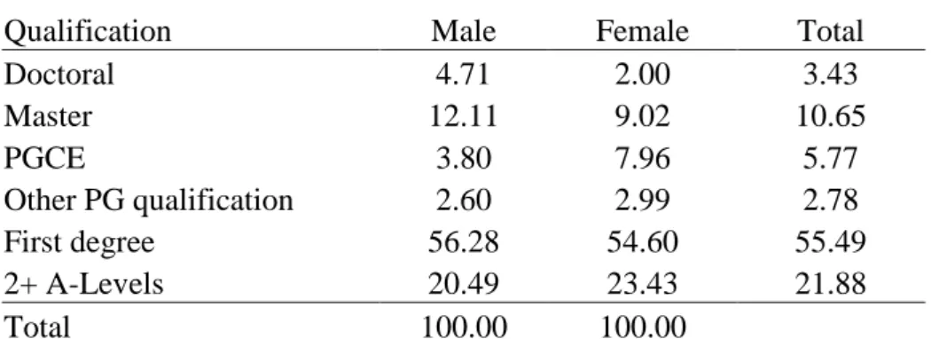
Our estimation uses a large sample of graduates (i.e. individuals in the data have successfully completed a first degrees) together with individuals who do not have a degree but who completed high school and attained sufficient qualifications to allow them, in principle, to attend university. We think of the latter group as our controls. The data is drawn from the Labour Forces Surveys – the LFS is the largest survey that UK National Statistics conduct, with slightly less than 1% of the population, and contains extensive information about labour market variables at the individual level. We drop all observations who did not achieve high school graduation with the level of qualifications to enter university – i.e. less than 2 A-level qualifications. In the UK, HE entry is rationed by achievement recorded at the end of high school and those without the absolute minimum achievements to attend university are excluded here³. We also drop Scotland and Northern Ireland residents and recent immigrants who were educated outside the UK. We use data pooled from successive Labour Force Surveys from 1994 (although information about class of degree was first collected only from 2005) to 2009 (the latest currently available). The resulting sample size of 25-60 year olds is 82,002. Wage data is derived from earnings and hours of work (converted to January 2010 prices using the RPI). Importantly for this work, LFS is a (albeit short) panel dataset from 1997 onwards. Postgraduate qualifications are categorised as either Masters level, PhD level, PGCE (a one year professional training for those entering teaching), and Other (we believe this will be largely qualifications associated with professional training that results in membership of chartered institutes and degrees such as MBA). Table 1 shows the simple breakdown of by gender and postgraduate qualification and Table 2 shows the corresponding average log wages. Women are twice as likely to have PGCE’s as men, but less likely to have Master or Doctoral degrees. Overall 29% of graduates in our data have postgraduate qualifications and around half of these are to Masters level. Average hourly wage differentials are pronounced: males (females) with first degrees only earn 20% (31%) more than those with 2+ A-levels only – reflecting the lower gender discrimination in the graduate labour market; males (females) with a Masters degree earn 12 % (17%) more than those with a first degree alone; male (female) PhDs earn 4% (7%) more than Masters; male (female) PGCEs earn 6% less (7% more) than those with first degrees alone.

3 We would like to be able to test the stability of our estimates to this threshold but this is, unfortunately, all the data will allow us to do.

Table 1 Distribution of Highest Qualifications by Gender, %

Qualification Male Female Total

Doctoral 4.71 2.00 3.43

Master 12.11 9.02 10.65

PGCE 3.80 7.96 5.77

Other PG qualification 2.60 2.99 2.78

First degree 56.28 54.60 55.49

2+ A-Levels 20.49 23.43 21.88

Total 100.00 100.00

Table 2 Mean Log Wages by Highest Qualification and Gender

Qualification Male Female Total

Doctoral 3.035 2.902 2.999

Master 2.991 2.831 2.927

PGCE 2.824 2.734 2.765

Other PG qualification 2.957 2.784 2.869

First degree 2.881 2.662 2.779

2+ A-Level 2.684 2.350 2.515

Total 2.861 2.618 2.746

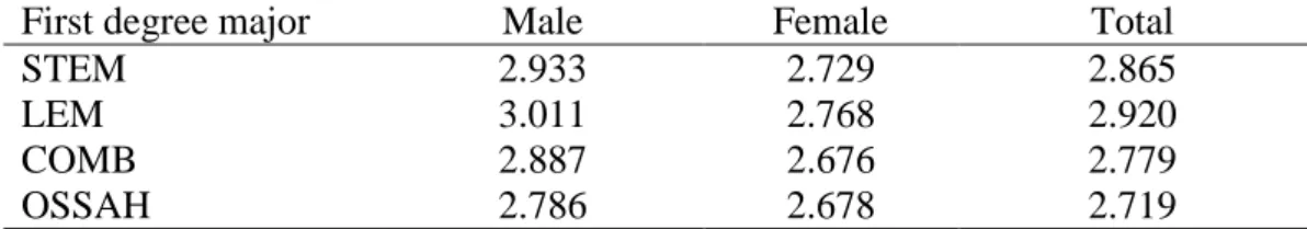
In the UK it is common for undergraduate students to study only a single subject – although this tendency is becoming less pronounced over time. Undergraduate degrees in the data are categorised into 12 subject areas which we, for reasons of sample size, collapse into four broad subject groups: STEM (Science, Technology, Engineering and Medicine which includes mathematics⁴

Table 3 shows the simple breakdown of log wage by gender and first degree subject of major. The average college premium for OSSAH majors relative to 2+ A-levels (in Table 3) is 10% (33%) for males (females); while for COMB it is 20% (33%) for males (females);

for STEM it is 25% (38%) for males (females); and for LEM it is 33% (42%) for males (females). Table 3 is for all graduates, but similar differentials are obtained just looking at those with a first degree alone.

); LEM (Law, Economics and Management), OSSAH (other social sciences, arts and humanities which includes languages), and COMB (those with degrees that combine more than one subject - but we do not know what these combinations are in our data).

4 We have grouped architects and graduate nurses into STEM, although their sample size is small enough for this to make no difference to our broad conclusions.

In the UK first degrees are classified by rank: first class (9.7% of non-missing degrees), upper second class (45.5%), lower second class (33.8%), third class (5.0%) and pass (6.1%). Table 4 shows the simple breakdown of log wage by gender and class of first degree. The premium for an upper second class degree over a lower second degree or worse is 8% (6%) for males (females), and the premium for a first over an upper second is 4% (5%) for males (females).

Table 3 Mean Log Wages by First Degree Major by Gender: All Graduates

First degree major Male Female Total

STEM 2.933

3.011 2.887 2.786

2.729 2.768 2.676 2.678

2.865 2.920 2.779 2.719 LEM

COMB OSSAH

Table 4 Mean Log Wages by First Degree Class by Gender: All Graduates

First degree class Male Female Total

First class 2.988 2.778 2.884

Upper second 2.948 2.724 2.821

Below upper second 2.869 2.665 2.770

Degree class missing 2.937 2.754 2.847

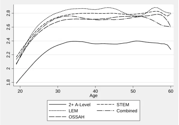
Figures 1 and 2 shows the observed relationship between log wages and age for A- level students and by degree major for men and women respectively. We use local regression methods to smooth the relationship. There are very clear differences between graduates and non-graduates and these differences vary by age for both men and women. There are also differences between majors for graduates which again differ by age. Age-earnings profiles differ and the differences are complicated: they do not appear to be parallel, which is what typical specifications assume. The figure for males suggests that the usual quadratic specification for the age-earnings profile would be a reasonable approximation to the data – but that a single quadratic relationship would be unlikely to fit each major equally well. For example, male LEM students enjoy faster growth in wages early in the lifecycle compared to other majors including STEM. There is no single college premium: wage premia seem to differ by major and by age.

These figures suggest that econometric analysis will need to be sufficiently flexible to capture these differences across majors. Moreover, Figure 2 looks quite different from Figure 1. The age-earnings profiles for women are much flatter - age is a poorer proxy for work experience for women because of time spent outside the labour market. This suggests that the

conventional cross-section methods are probably not going to be able to provide a good guide to how the earnings of women evolve over the lifecycle.

Figure 1 Smoothed Local Regression Estimates of Age – Log Earnings Profiles: Men

Figure 2 Smoothed Local Regression Estimates of Age – Log Earnings Profiles: Women

1.522.533.5

20 30 40 50 60

Age

2+ A-Level STEM

LEM Combined

OSSAH

1.822.22.42.62.8

20 30 40 50 60

Age

2+ A-Level STEM

LEM Combined

OSSAH

3. Method and Estimates

The conventional approach to estimating the private financial return to education typically uses a simple specification such as:

(1) logw_i = +α βExperience_i+γExperience_i²+δX χQ_i+ _i+e_i for i=1..N

where X is a vector of individual characteristics such as migrant status and region of residence, and Q is a vector that records qualifications but, in many studies, simply measures years of completed full-time education. Age is often used as a proxy for work experience.

Here, we focus on graduates, postgraduates and a subset of non-graduates (those that could, in principle, have attended university) and allow differentiation by major studies in Q.

Using a control group that consists of those who might have attended university seems likely to reduce the impact of ability bias on our estimates, and so get us closer to estimating causal effects, although it seems unlikely that it would eliminate it altogether and this needs to be borne in mind when interpreting the estimates.

Our estimates of such a simple specification as (1) reflect the stylised facts that we reported in Section 2 and are not reported here. Rather, since we wish to use our estimates to inform public policy we need to ensure that the specification has the flexibility to reflect the policy issues as well as the realities of the raw data. Section 2 strongly suggests that we should not impose parallel age – earnings profiles so we will provide estimates broken down by highest qualification: that is, separate estimates for those with 2+ A-levels from those with STEM first degree, LEM, etc. That is, we would prefer to estimate

(2) logw_iq = +α β_qExperience_i+γ_qExperience_i² +δ X_{q i}+e_iq for i=1.. and N q=0..4 which does not impose age earnings profiles to be parallel in q, qualification.

There are two further difficulties. First, as we saw in Section 2, age is a poor proxy for work experience for women. If we wish to model how wages evolve over the lifecycle conditional on continuous participation estimating such a cross section model is not likely to be helpful. The second problem is that it seems likely that there are cohort effects on wages and identifying cohort effects separately from lifecycle effects is impossible with a single cross-section of data and problematic with pooled cross sections over a relatively short span of time. We can resolve both of these difficulties by exploiting the panel element of the data.

If we time difference equation (2) we obtain

(3) ∆logw_iq =β_q+2γ_qExperience_i+u_iq for i=1.. and N q=0..4

which allows us to estimate the parameters of the age-earnings profiles, by major (and for the 2+ A-level group) separately from cohort effects providing such cohort effects are additive in equation (2). Indeed, it seems likely that differencing will eliminate some of the unobservable determinants of wage levels that might otherwise contaminate the estimates of the age earnings profile. This then provides independent panel data estimates that can then be imposed in equation (2) which can then be estimated on the pooled cross section data.

Moreover, panel data estimation for employed women provides estimates that are likely to be much closer to the effects of experience. That is, we can then estimate

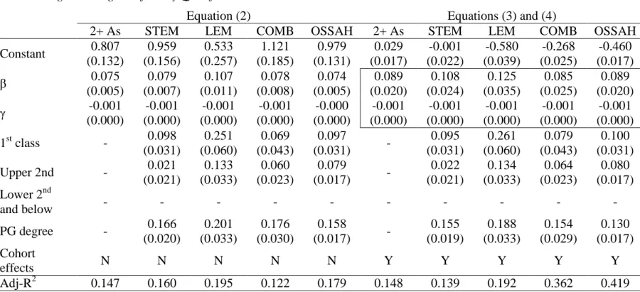
(4) logw_iq =α( )c_i +βˆ_qExperience_i+γˆ_qExperience_i²+δ X_{q i}+v_iq for i=1.. and N q=0..4 from the pooled cross-section data. Tables 5a (men) and 5b (women) report our baseline OLS pooled cross-section estimates of equation (2) without cohort effects; together with estimates of (3), from the panel, and (4) from the pooled cross sections which include additive cohort effects (we include a cubic in year of birth)⁵. For men, in Table 5a, we find that the estimated lifecycle age-earnings parameters, the γ’s and β’s, are reassuringly similar for men whether estimated using the pooled cross-section estimates of the levels equations or from the panel data estimation of the wage difference equations. Nonetheless we find statistically important cohort effects when we impose the lifecycle coefficients from the panel estimation on the pooled cross section estimation of the levels equations. However, for women in Table 5b, we find that the panel estimation provides much steeper age earnings profile estimates – the estimated β’s are, on average, approximately 20% higher than those found in the pooled cross section estimates of the levels equation. Moreover, there are larger differences in profiles across majors. Thus, separating the estimation of lifecycle and cohort effects is important, at least for women. The estimates age-experience profiles are plotted in Appendix Figures A1a and A1b - for men the profile for LEM starts higher and is steeper and dominates all other subjects until late in the lifecycle when COMB catches up; for women, OSSAH and COMB are very close but, while other subjects are slightly higher at an early age, their profiles are flatter⁶

5 We also include controls for region and immigrant status which are not reported but there are no significant

differences in the estimates when we include them. We find that our estimates of the crucial effects are not affected by aggregating the PG qualifications so we group all PG qualifications into a single variable to capture the average effect across all PG qualifications.

.

6 See Appendix Table A7’ for NPVs based on these estimated age-earnings profiles for full-time workers alone.

We have included degree class and postgraduate degrees in the specification as simple intercept shifts and we find important differences across subjects. There is a significant premium for degree class that varies across majors: there are particularly large effects for LEM graduates for both men and women; although the differences between first class and upper second class are generally not significant. There is an effect of having PG qualifications over and above the effect of degree class: with PG premia at around 15% in all subjects for women. For men, the corresponding PG premia range between 5-10%, with higher returns for LEM and COMB.

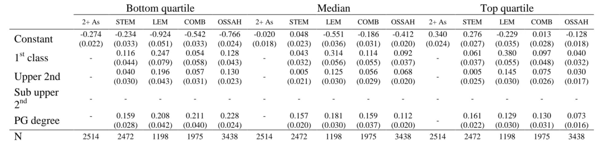
Tables 6a and 6b reports Quantile Regression results for equation (4) (where the estimated experience-earnings profile is drawn from OLS estimates of the wage growth equation using the panel data). Our motivation for investigating the effect of HE across quantiles of the residual wage distribution is the presumption that the latter captures the distribution of unobserved skills. Thus, it is of interest to estimate the effect of HE across this distribution. It is difficult to predict what these effects might look like. On the one hand one might argue that unobserved skills, like perseverance, might complement observed skills (like a specific HE qualification) and that we would therefore expect the Net Present Value (NPV) of a HE qualification to be higher at the top of the distribution than at the bottom. Indeed, low unobserved skills associated with poor high school performance would typically be associated with admission to a low ranked institution that may add less value than a higher rated institution. On the other hand, one might argue that those with poor unobserved skills might attempt to compensate for them by investing (unobserved) greater effort as an undergraduate student. In which case, we might see higher returns at the bottom of the distribution of unobserved skills.

The male premium for a first class is close to 10% across the quartiles for STEM, and the results for women are similar. The upper second premia are also close to 10% for STEM men, but are not significantly different from zero for women. The male LEM first class premia are large for the bottom quartile at 25% and similar for the median, but somewhat smaller for the upper quartile. The LEM bottom quartile female first class premium is very similar to the male premium and are over 30% for the median and top quartile. The LEM upper second premia is slightly smaller than the first premia for men, while for women they are similar to the male premium at the bottom decile but around 15% for the median and top quartile. The upper second effects for COMB men is small across the distribution; and the

Table 5a Estimated Age Earnings Profiles by Qualification: Men

Equation (2) Equations (3) and (4)

2+ A’s STEM LEM COMB OSSAH 2+ A’s STEM LEM COMB OSSAH

Constant 0.158 (0.154)

0.435 (0.138)

-0.103 (0.254)

0.105 (0.225)

0.200 (0.200)

-0.537 (0.019)

-0.339 (0.017)

-1.407 (0.033)

-1.051 (0.028)

-0.567 (0.024)

β 0.119

(0.006)

0.107 (0.006)

0.138 (0.011)

0.129 (0.009)

0.108 (0.008)

0.121 (0.021)

0.107 (0.018)

0.168 (0.031)

0.116 (0.027)

0.131 (0.027)

γ -0.001

(0.000)

-0.001 (0.000)

-0.001 (0.000)

-0.001 (0.000)

-0.001 (0.000)

-0.001 (0.000)

-0.001 (0.000)

-0.002 (0.000)

0.001 (0.000)

-0.001 (0.000)

1^st class - 0.075

(0.025)

0.236 (0.062)

0.139 (0.054)

0.040

(0.046) - 0.075

(0.025)

0.236 (0.062)

0.141 (0.054)

0.047 (0.046)

Upper 2^nd - 0.090

(0.018)

0.185 (0.034)

0.053 (0.029)

0.050

(0.025) - 0.088

(0.017)

0.182 (0.034)

0.053 (0.029)

0.052 (0.025) Lower 2^nd

and below - - - -

PG degree - 0.066

(0.018)

0.094 (0.031)

0.121 (0.034)

0.072

(0.026) - 0.050

(0.017)

0.086 (0.030)

0.106 (0.034)

0.065 (0.025) Cohort

effects N N N N N Y Y Y Y Y

Adj-R² 0.311 0.242 0.226 0.211 0.214 0.142 0.257 0.189 0.452 0.127

Notes: Region and immigrant controls and missing degree class included. Standard errors in parentheses.

Table 5b Estimated Age Earnings Profiles by Qualification: Women

Equation (2) Equations (3) and (4)

2+ As STEM LEM COMB OSSAH 2+ As STEM LEM COMB OSSAH

Constant 0.807 (0.132)

0.959 (0.156)

0.533 (0.257)

1.121 (0.185)

0.979 (0.131)

0.029 (0.017)

-0.001 (0.022)

-0.580 (0.039)

-0.268 (0.025)

-0.460 (0.017)

β 0.075

(0.005)

0.079 (0.007)

0.107 (0.011)

0.078 (0.008)

0.074 (0.005)

0.089 (0.020)

0.108 (0.024)

0.125 (0.035)

0.085 (0.025)

0.089 (0.020)

γ -0.001

(0.000)

-0.001 (0.000)

-0.001 (0.000)

-0.001 (0.000)

-0.000 (0.000)

-0.001 (0.000)

-0.001 (0.000)

-0.001 (0.000)

-0.001 (0.000)

-0.001 (0.000)

1^st class - 0.098

(0.031)

0.251 (0.060)

0.069 (0.043)

0.097

(0.031) - 0.095

(0.031)

0.261 (0.060)

0.079 (0.043)

0.100 (0.031)

Upper 2nd - 0.021

(0.021)

0.133 (0.033)

0.060 (0.023)

0.079

(0.017) - 0.022

(0.021)

0.134 (0.033)

0.064 (0.023)

0.080 (0.017) Lower 2^nd

and below - - - -

PG degree - 0.166

(0.020)

0.201 (0.033)

0.176 (0.030)

0.158

(0.017) - 0.155

(0.019)

0.188 (0.033)

0.154 (0.029)

0.130 (0.017) Cohort

effects N N N N N Y Y Y Y Y

Adj-R² 0.147 0.160 0.195 0.122 0.179 0.148 0.139 0.192 0.362 0.419

Notes: Region and immigrant controls and missing degree class included. Standard errors in parentheses.

Table 6a Quantile Regression results: Men

Bottom quartile Median Top quartile

2+ As STEM LEM COMB OSSAH 2+ As STEM LEM COMB OSSAH 2+ As STEM LEM COMB OSSAH

Constant _(0.027) ^-0.920 _(0.019) ^-0.574 _(0.032) ^-1.663 _(0.041) ^-1.332 _(0.028) ^-0.840 _(0.022) ^-0.484 _(0.016) ^-0.309 _(0.035) ^-1.412 _(0.027) ^-1.021 _(0.027) ^-0.530 _(0.024) ^-0.156 _(0.021) ^-0.062 _(0.043) ^-1.036 _(0.034) ^-0.694 _(0.027) ^-0.260 1^st class ^- _(0.029) ^0.092 _(0.063) ^0.243 _(0.079) ^-0.003 _(0.053) ^{0.007 -} _(0.024) ^0.102 _(0.064) ^0.231 _(0.052) ^0.110 _(0.051) ^{0.093 -} _(0.030) ^0.089 _(0.078) ^0.208 _(0.066) ^0.149 _(0.050) ^0.085 Upper 2nd ^- _(0.020) ^0.103 _(0.034) ^0.157 _(0.042) ^0.014 _(0.029) ^{0.002 -} _(0.017) ^0.098 _(0.035) ^0.225 _(0.028) ^0.018 _(0.027) ^{0.076 -} _(0.021) ^0.082 _(0.042) ^0.168 _(0.035) ^0.060 _(0.027) ^0.103 Sub upper

2^{nd - - - - - - - - - - - - -}

PG degree ^- _(0.021) ^0.043 _(0.031) ^0.092 _(0.051) ^0.194 _(0.030) ^{0.158 -} _(0.017) ^0.027 _(0.032) ^0.071 _(0.033) ^0.128 _(0.028) ^{0.070 -} _(0.021) ^0.057 _(0.038) ^0.110 _(0.039) ^0.090 _(0.029) ^0.049

N ^{2202 3668 1405 1474 1807 2202 3668 1405 1474 1807 2202 3668 1405 1474 1807}

Note: Estimates of β and γ are imposed from the right hand blocks of Table 5a. Cohort effects are included throughout. Region and immigrant controls and missing degree class also included. Standard errors in parentheses.

Table 6b Quantile Regression results: Women

Bottom quartile Median Top quartile

2+ As STEM LEM COMB OSSAH 2+ As STEM LEM COMB OSSAH 2+ As STEM LEM COMB OSSAH

Constant _(0.022) ^-0.274 _(0.033) ^-0.234 _(0.051) ^-0.924 _(0.033) ^-0.542 _(0.024) ^-0.766 _(0.018) ^-0.020 _(0.023) ^0.048 _(0.036) ^-0.551 _(0.031) ^-0.186 _(0.020) ^-0.412 _(0.024) ^0.340 _(0.027) ^0.276 _(0.035) ^-0.229 _(0.028) ^0.013 _(0.018) ^-0.128 1^st class ^- _(0.044) ^0.116 _(0.079) ^0.247 _(0.058) ^0.054 _(0.043) ^{0.128 -} _(0.032) ^0.043 _(0.056) ^0.314 _(0.055) ^0.114 _(0.037) ^{0.092 -} _(0.037) ^0.061 _(0.055) ^0.380 _(0.048) ^0.097 _(0.032) ^0.040 Upper 2nd ^- _(0.030) ^0.040 _(0.043) ^0.196 _(0.031) ^0.057 _(0.023) ^{0.130 -} _(0.021) ^0.005 _(0.030) ^0.125 _(0.029) ^0.056 _(0.020) ^{0.068 -} _(0.025) ^0.005 _(0.030) ^0.145 _(0.026) ^0.075 _(0.017) ^0.030 Sub upper

2^{nd - - - - - - - - - - - - - - -}

PG degree ^- _(0.028) ^0.159 _(0.042) ^0.208 _(0.040) ^0.211 _(0.024) ^{0.228 -} _(0.020) ^0.157 _(0.030) ^0.181 _(0.037) ^0.159 _(0.020) ^{0.112 -} _(0.022) ^0.161 _(0.030) ^0.129 _(0.031) ^0.130 _(0.016) ^0.073

N ^{2514 2472 1198 1975 3438 2514 2472 1198 1975 3438 2514 2472 1198 1975 3438}

Note: Estimates of β and γ are imposed from the right hand blocks of Table 5b. Cohort effects are included throughout. Region and immigrant controls and missing degree class included. Standard errors in parentheses.

same is true for women. The first class effect for OSSAH is badly determined for men, while for women there is a 13% effect at the bottom, 9% at the median, but insignificant at the top.

The PG effect is small for STEM men across the quartiles, but around 15% for STEM women across the quartiles. The PG effect for LEM males is 9% for the bottom quartile, slightly lower at the median and slightly higher at the upper quartile; while for women, the effect is 20% at the bottom, lower at the median and about half at the upper quartile. The effect of COMB women is in the mid to upper teen, and somewhat lower for men. The effect for OSSAH is 14% for men at the lower quartile, half this at the median, and half again at the upper quartile. A similar pattern holds for OSSAH women but from a higher level.

4. Lifetime impacts and rates of return

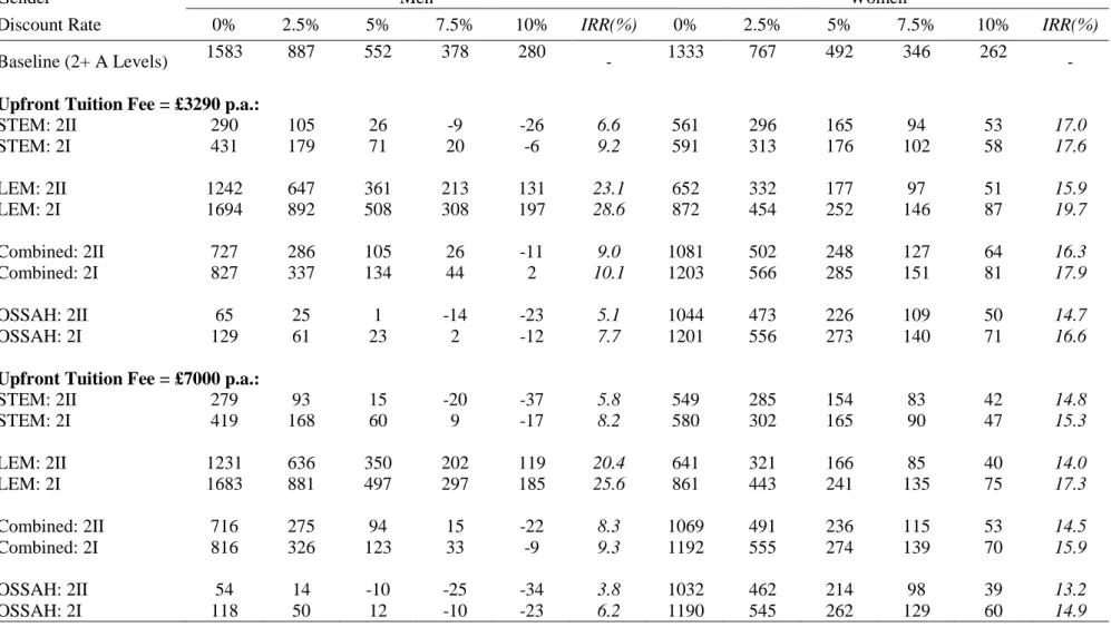
The implied college premia will vary with experience, degree class, cohort, and presence of PG qualifications⁷. Thus, in Table 7 we present, using the estimates of equations (3) and (4) from Tables 5a and 5b, the NPVs associated with a lifetime (from 22 to 65) with each major and a lifetime with 2+ A-levels (from 19 to 65) using various discount rates. We also include the internal rate of return (IRR), obtained from grid search. The assumption throughout is that there are tuition fees of either £3,290 (the level for 2010/11) or £7,000 pa for three years and opportunity costs are the (discounted) net of tax earnings that they would have received had they not entered university (i.e. those given by the estimates for 2+ A- levels) from 19 to 21. We allow for income taxes and employee social security contributions using the 2010 schedules⁸. We assume that individuals intend to work full-time throughout their working age lives⁹

7 Surprisingly, we find that the effects of qualifications do not differ across regions. In particular, the impact of major does not vary across regions: which is surprising given the concentration of LEM majors in London.

. We view this as a prospective simulation and focus on a current cohort looking forward. The simulations in Table 7 are for an “up-front” fee scheme since it does not allow for the presence of a loan scheme. In Table 10 and Appendix Table A7 we make allowance for this. To the extent that this scheme allows students to shift their tuition costs forward in time with no virtually interest penalty (and that the scheme contains an element of debt forgives) we are underestimating the NPVs (except when the discount rate is zero) and IRRs in Table 7. However, even at a 10% discount rate the differences in NPVs in Table A7 compared to Table 7 are proportionately very small - just 3 to 4 thousand pounds.

8 Welfare programmes and the minimum wage are hardly relevant over the range of data being considered here.

9 One might also want to incorporate some part of subsistence costs while studying. For example, many UK students study away from home and incur additional housing costs.

Table 7: NPVs relative to 2+ A-levels (£,000) and IRRs (%)) by Gender, Major, Degree Class, and Discount Rate

Gender Men Women

Discount Rate 0% 2.5% 5% 7.5% 10% IRR(%) 0% 2.5% 5% 7.5% 10% IRR(%)

Baseline (2+ A Levels) 1583 887 552 378 280

- 1333 767 492 346 262

-

Upfront Tuition Fee = £3290 p.a.:

STEM: 2II 290 105 26 -9 -26 6.6 561 296 165 94 53 17.0

STEM: 2I 431 179 71 20 -6 9.2 591 313 176 102 58 17.6

LEM: 2II 1242 647 361 213 131 23.1 652 332 177 97 51 15.9

LEM: 2I 1694 892 508 308 197 28.6 872 454 252 146 87 19.7

Combined: 2II 727 286 105 26 -11 9.0 1081 502 248 127 64 16.3

Combined: 2I 827 337 134 44 2 10.1 1203 566 285 151 81 17.9

OSSAH: 2II 65 25 1 -14 -23 5.1 1044 473 226 109 50 14.7

OSSAH: 2I 129 61 23 2 -12 7.7 1201 556 273 140 71 16.6

Upfront Tuition Fee = £7000 p.a.:

STEM: 2II 279 93 15 -20 -37 5.8 549 285 154 83 42 14.8

STEM: 2I 419 168 60 9 -17 8.2 580 302 165 90 47 15.3

LEM: 2II 1231 636 350 202 119 20.4 641 321 166 85 40 14.0

LEM: 2I 1683 881 497 297 185 25.6 861 443 241 135 75 17.3

Combined: 2II 716 275 94 15 -22 8.3 1069 491 236 115 53 14.5

Combined: 2I 816 326 123 33 -9 9.3 1192 555 274 139 70 15.9

OSSAH: 2II 54 14 -10 -25 -34 3.8 1032 462 214 98 39 13.2

OSSAH: 2I 118 50 12 -10 -23 6.2 1190 545 262 129 60 14.9

Table 8: Quantile Regression Estimates of NPVs (graduates are all relative to 2+ A-levels) at 5% Discount Rate, £,000.

Gender Men Women

Quantile 25^th 50^th 75th 25^th 50^th 75th

Baseline (2+ A Levels) 580 517 483 615 491 384

Tuition Fee = £3290 p.a.:

STEM: 2II -111 16 161 -42 124 314

STEM: 2I -72 60 212 -18 123 314

LEM: 2II 110 235 44 -29 -34 89

LEM: 2I 215 374 111 70 13 152

Combined: 2II 136 62 -43 30 223 350

Combined: 2I 148 80 -17 49 257 389

OSSAH: 2II -175 -47 84 9 163 370

OSSAH: 2I -178 -20 117 78 201 391

Tuition Fee = £7000 p.a.:

STEM: 2II -122 5 150 -53 112 303

STEM: 2I -83 49 201 -30 112 302

LEM: 2II 99 223 33 -41 -45 78

LEM: 2I 204 363 100 58 2 141

Combined: 2II 125 51 -54 18 212 339

Combined: 2I 137 69 -28 38 245 378

OSSAH: 2II -186 -59 73 -2 152 359

OSSAH: 2I -189 -31 106 67 190 380

Table 9: Internal Rate of Returns (IRRs) for Quantile Regression Estimates of NPVs, %.

Gender Men Women

Quantile 25^th 50^th 75th 25^th 50^th 75th

Baseline (2+ A Levels) - - - - - -

Tuition Fee = £3290 p.a.:

STEM: 2II <0 6.0 15.3 0.8 14.4 27.8

STEM: 2I <0 8.9 18.2 3.4 14.4 27.8

LEM: 2II 11.6 18.6 8.5 3.0 2.0 11.7

LEM: 2I 16.5 24.6 12.8 8.8 6.0 15.8

Combined: 2II 10.0 7.6 2.9 6.1 15.2 23.5

Combined: 2I 10.4 8.4 4.2 6.8 16.7 25.4

OSSAH: 2II <0 <0 13.4 5.3 12.1 23.5

OSSAH: 2I <0 0.5 15.9 7.7 13.6 24.4

Tuition Fee = £7000 p.a.:

STEM: 2II <0 5.3 13.2 0.2 12.5 23.8

STEM: 2I <0 7.8 15.7 2.7 12.5 23.8

LEM: 2II 10.3 16.3 7.3 2.5 1.4 10.1

LEM: 2I 14.7 21.6 11.1 7.9 5.1 13.7

Combined: 2II 9.2 6.9 2.5 5.6 13.6 20.3

Combined: 2I 9.5 7.6 3.8 6.3 14.9 21.9

OSSAH: 2II <0 <0 11.3 4.9 10.9 20.4

OSSAH: 2I <0 <0 13.5 7.1 12.3 21.2

The IRRs are large for women for all majors and for both good and bad degrees. This increase in tuition fee, on the scale envisaged in the Browne Report, makes a not economically insignificant dent in the IRR - around 2 to 2.5%. The differences across majors are quiet small. For men, there is substantially more variation. The return to LEM is large for both good and bad degrees, and the tuition fee rise makes a sizeable difference of around 3%.

STEM, Combined and OSSAH all return modest levels according to the calculated IRRs.

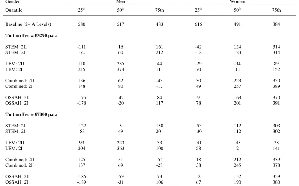
In Table 8 we use the corresponding estimates from Tables 6a and 6b to show how the NPV results vary by quantile of the distribution at a given discount rate, 5%, by gender, degree class and major. The median figures in Table 8 are close to the average figures that OLS yields in Table 7. However, there are huge differences across the quantiles within Table 8. Even for women, it would appear that the effects of STEM on NPV at the bottom quartile are much lower and even negative. At higher fees even the LEM median goes negative for women. Huge negative effects are associated with OSSAH for men. Note that the table demonstrates NPVs that rise across the distribution in some cases but not all. For example, for STEM and OSSAH, NPVs rise as we move up the distribution, but the opposite is true for Combined. There is no strongly theoretical presumption that any particular pattern should manifest itself and the estimates allow for all possibilities. Table 9 translates the NPV findings across the quantiles into rates of return. This confirms the relatively modest effects of the tuition rise on the returns on student investments. Those subjects that offer low returns at fees of £3290, offer somewhat lower returns at fees of £7000. Subjects that offer high returns at £3290 suffer larger falls if fees rise to £7000, but still offer handsome returns.

We also analyse the impact of the additional maintenance costs that might reasonably be associated with higher education participation. It would not be appropriate for all of subsistence expenditure during studying for a degree to be counted as an opportunity cost – only that expenditure that is over and above what would normally be spent had the individual not attended university. We know little about what these expenditures might be but a convenient figure would be £3250 p.a. (say £2800 p.a. for rent¹⁰

10 £70 per week for 30 weeks plus half rent for the summer vacation.

and £450 p.a. for study materials). Under the current loan scheme students from low income backgrounds are eligible to a maximum maintenance grant of £2906 pa, while students from higher income backgrounds are eligible to a loan to cover such costs. So, in Table 10, we simulate the effect of adding this expenditure to the opportunity costs of a degree and the comparison between two adjacent columns tells us about the value of being eligible to a grant, as opposed to a

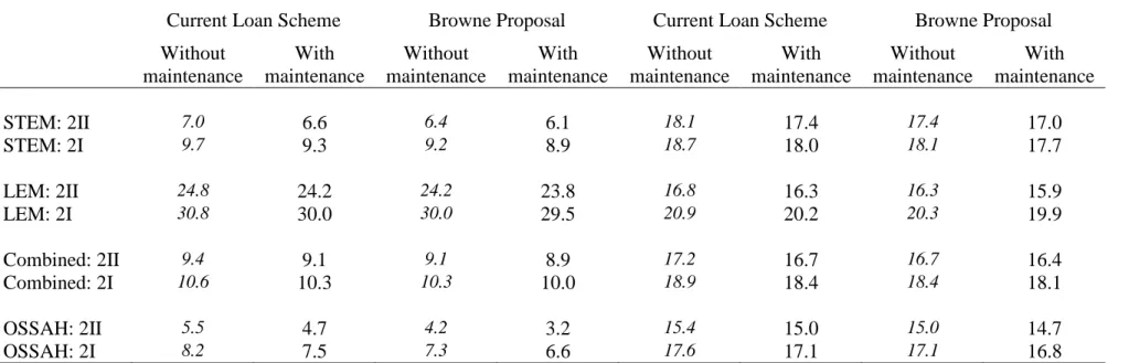
loan, to cover such spending. That is, the column headed “without maintenance” assumes that there is a grant to cover such costs, (i.e. this corresponds to a student from a low income household) while the column headed “with maintenance” assumes that students borrow (i.e from a higher income household). Comparing the figures for the current loan scheme in Table 10 for those “without maintenance” (i.e. whose maintenance cost are covered by a grant) with the figures in the top half of Table 7 we see the effect of this additional expenditure makes very little difference to the IRR. Having to borrow to cover this maintenance expenditure (comparing the first and second columns of Table 10 for men, and the fifth and sixth form women) rather than having a grant to cover this, lowers the IRR - but by less than one percentage point in all cases. Figure 10 also simulates a version of the proposals put forward by the Browne Review (Browne, 2010). In those proposals a fee level of £7000 becomes a focal point (as opposed to the current £3290) and we adopt the other proposals – an interest rate of 2.2% (as opposed to zero), debt write off after 30 years (rather than 25), and payable at 9% of earnings above £21,000 p.a. (as opposed to £15,000). The results suggests a small, almost always less than one percentage point, fall in the IRR.

5. Conclusion

This paper has used the latest and largest dataset available to estimate as flexible specification as possible. We allowed for tuition fees and the tax system in calculating the NPV associated with higher education (and also the loan scheme). And we provide independent estimates for graduates with different degree majors. The results are large for women - reflecting the greater discrimination that women face in the sub-degree labour market. Indeed, they are large across the board.

The results for men vary considerably across majors: with LEM having very large returns for both good and bad degrees, although higher tuition fees knock around 3% off these figures. The return to STEM is around 7% for a bad degree and 9% for a good one;

COMB degrees are slightly higher; while OSSAH degrees are only 5% in the case of a bad degree. The first notable feature of the results is that the scale of tuition fee rise envisaged does not change the relative IRRs across subjects very much. Such rises are dwarfed by the scale of life earnings differentials. These results suggest that we might not see much substitution across majors in the face of even quite large tuition fee changes¹¹

11 Arciadiacono et al (2010) provide estimates of the sensitivity of choice of college major to perceptions of differentials in returns of the US. No such research is available for the UK.

. The second feature is that, while there is little variation in returns across majors for women, STEM

subjects do not seem to exhibit large returns for men. They are dominated by COMB degrees and vastly so by LEM degrees. Indeed, if we imagined that the IRR reflected relative scarcity there would not seem to be a compelling case for thinking that there was a STEM shortage.

On the contrary, there would seem to be a case for wanting to encourage a switch from OSSAH to LEM for men. The results are, of course, simulations using averages. There is likely to be wide variation around the averages and this is confirmed when we use Quantile Regression to look across quantiles of the residual log wage distribution. The best way to think of these quantiles is differences in wages that reflect unobservable differences across individuals. We might imagine that the prime suspect behind these unobservable effects is

“ability” – there is likely to be wide variation across individuals in their unobserved abilities to make money. This will be conflated with institutional effects and family background – low ability students are likely to attend lower perceived quality institutions. Unfortunately, we have no way of knowing how much of the large variation in returns across quantiles is due to individual differences and how much because of institutional differences. Only richer data will allow us to address this point.

However, we find consistently strong returns to a 2.1 vs a 2.2 – it would appear that, in all subjects, there is a strong return to effort. A good degree raises the IRR, ranging from 1% to 5.5% - although we are unable to say how much effort is required to generate such a better degree result¹²

Finally, a rise in tuition fees to £7000 would lower returns by about 1-3% - not economically insignificant. The strong message that comes out of this research is that even a large rise in tuition fees makes relatively little difference to the quality of the investment – those subjects that offer high returns (LEM for men, and all subjects for women) continue to do so. And those subjects that do not (especially OSSAH for men) will continue to offer poor returns. The Browne Report proposes slightly lower fees (£7000 is a focal point of the report) than originally envisaged but suggests an unsubsidized interest rate (of 2.2%) which is repayable only when incomes exceed a higher threshold (£21,000 rather than £15,000). Our analysis suggests that this proposal would have somewhat more modest detrimental effects on the soundness of an investment in higher education - but large cross subject differences will remain.

.

12 Strinebricker and Strinebricker (2009) show that effort has a large effect on US degree scores – the GPA. We know of no UK work on this topic.

Table 10: A Comparison of IRRs (relative to A-levels) under Current Scheme and Browne Proposal, %

MEN WOMEN

Current Loan Scheme Browne Proposal Current Loan Scheme Browne Proposal Without

maintenance

With maintenance

Without maintenance

With maintenance

Without maintenance

With maintenance

Without maintenance

With maintenance

STEM: 2II 7.0 6.6 6.4 6.1 18.1 17.4 17.4 17.0

STEM: 2I 9.7 9.3 9.2 8.9 18.7 18.0 18.1 17.7

LEM: 2II 24.8 24.2 24.2 23.8 16.8 16.3 16.3 15.9

LEM: 2I ^30.8 30.0 ^30.0 29.5 ^20.9 20.2 ^20.3 19.9

Combined: 2II 9.4 9.1 9.1 8.9 17.2 16.7 16.7 16.4

Combined: 2I ^10.6 10.3 ^10.3 10.0 ^18.9 18.4 ^18.4 18.1

OSSAH: 2II 5.5 4.7 4.2 3.2 15.4 15.0 15.0 14.7

OSSAH: 2I 8.2 7.5 7.3 6.6 17.6 17.1 17.1 16.8

Notes: Current loan scheme: Fee of £3290, 0% real interest rate, repayment on 9% of annual earnings over £15k and writing-off after 25 years; Browne Proposal: Fee of £7000, 2.2% real interest rate, repayment on 9% of annual earnings over £21k and writing-off after 30 years; Maintenance: £2906 (£3250) added to tuition fees under current loan scheme (Browne Proposal).

References

Arciadiacono, P., V. Joseph Hotz, and S. Kang (2010), “Modelling college major choice using elicited measures of expectations and counterfactuals”, NBER WP 15729.

Blundell, R.W., L. Dearden and B. Sianesi, (2005), “Evaluating the impact of education on earnings: Models, methods and results from the NCDS”, Journal of the Royal Statistical Society Series A, 168, 473-512.

Browne, J (Lord Browne of Madingley), (2010), Securing a Sustainable Future for Higher Education”

Chevalier, A., (2009), ‘Does Higher Education Quality Matter in the UK?’ Royal Holloway, University of London, mimeo.

Dolton, P.J., G.D. Inchley and G.H. Makepeace (1990), “The early careers of 1980 graduates:

earnings, earnings differentials and postgraduate study”, UK Department of Employment Research Paper No. 78.

Dearden, L., A. Goodman, G. Kaplan and G. Wyness (2010), “Future arrangements for funding higher education”, IFS Commentary C115.

Eide, E., D. Brewer and R.G. Ehrenberg (1998). “Does It Pay to Attend an Elite Private College? Evidence on the Effects of Undergraduate College Quality on Graduate School Attendance”, Economics of Education Review, 17, 371–376.

Hoxby, C. (2009), “The Changing Selectivity of American Colleges”, NBER WP 15446.

Hussain, I., S. McNally, and S. Telhaj, (2009), “University Quality and Graduate Wages in the UK”, IZA WP 4043.

Sloane, P.J. and N.C. O'Leary (2005), “The Return to a University Education in Great Britain”, National Institute Economic Review, 193, 75-89

Strinebrickner, R. and T.R. Strinebrickner (2008), “The causal effect of studying on academic performance”, BE Journal of Economic Analysis and Policy, 8, 1-53.

Walker, I and Y. Zhu (2008), “The College Wage Premium and the Expansion of Higher Education in the UK”, Scandinavian Journal of Economics, 110, 695-709.

Appendix

The 82,002 observations in Section 2 is a sample of 25-60 year olds pooled from 1994-2009 Wave 5. This is effectively the same sample as was used in Walker and Zhu (2008), updated with 3 more years.

The cross-sectional estimation sample relaxes the age range to 19-60 (22-60 for graduates), with the sample size increased to 90,388.

The panel data is a panel of addresses and ensuring it is a panel of individuals results in some attrition. The wage panel is based on post 1997 LFS, N=43,545 which can be matched to almost 75% of the post-1997 cross-sectional sample.

The sample with degree class information is post-2005, N=22,153. This sample of 19- 60 (22-60 for graduates) year olds is the actual sample used for simulation. The age range 61- 65 in the simulation results are extrapolated from the 19-60 sample, but we think we are probably justified in doing so because of selectivity issues (too few women are still working above 60 and the differential pension age in public/private sectors for men).

Figure A1a: Estimated age - earnings profiles by subject (2II for graduates), men

Figure A1b: Estimated age - earnings profiles by subject (2II for graduates), women

22.533.544.5

20 25 30 35 40 45 50 55 60 65

age

2+ A-Level STEM

LEM Combined

OSSAH

2.533.544.5

20 25 30 35 40 45 50 55 60 65

age

2+ A-Level STEM

LEM Combined

OSSAH