How star cluster evolution shapes protoplanetary disc sizes
I n a u g u r a l - D i s s e r t a t i o n
zur
Erlangung des Doktorgrades
der Mathematisch-Naturwissenschaftlichen Fakult¨ at der Universit¨ at zu K¨ oln
vorgelegt von Kirsten Vincke
aus Arnsberg
K¨ oln
2019
Prof. Dr. Peter Schilke . . . .
Tag der m¨ undlichen Pr¨ ufung: 23.07.2018
Zusammenfassung
Die meisten Sterne entstehen nicht in Isolation, sondern als Teil von Gruppen, die zwischen einigen zehn bis mehreren hunderttausend Mitglieder enthalten k¨ onnen. Die Sterne entste- hen durch den Kollaps einer kalten Riesenmolek¨ ulwolke, wobei ein Anteil des Gases in der Molek¨ ulwolke in Sterne umgewandelt wird, w¨ ahrend der Rest sp¨ atestens einige Millionen Jahre nach Beginn der Sternentstehung aus der Sterngruppe ausgestoßen wird. Wurde weniger als 30% der Molek¨ ulwolkenmasse in Sterne umgewandelt, so wird hierbei ein Teil der Sterngruppe ungebunden. Entstehen allerdings Sterne aus mehr als 60% der Masse, bleibt die Sterngruppe gr¨ oßtenteils gebunden. Im ersten Fall spricht man von kurzlebigen
Assoziationen, in letzterem von langlebigen Sternhaufen, die sich zu Offenen Sternhaufenmit Lebensdauern von vielen Milliarden Jahren entwickeln k¨ onnen. Die beiden Typen von Sterngruppen unterscheiden sich sehr in ihren Eigenschaften und ihrer Entwicklung im Bezug auf Dichte und Gr¨ oße.
Jeder Stern, unabh¨ angig von der Art seiner Sterngruppe, ist von einer
protoplanetaren Scheibeumgeben, aus der sich potentiell Planeten bilden k¨ onnen. Bis heute wurden mehr als 3 700 Planeten entdeckt, die andere Sterne umkreisen. Viele dieser Planetensysteme unterscheiden sich allerdings stark von unserem Sonnensystem. In dieser Arbeit wird un- tersucht, inwieweit die Art der Sterngruppe, in der ein Stern entstanden ist, Einfluss auf die Gr¨ oße eines sich formenden Planetensystems haben kann. Zwei Prozesse, welche maßge- blich die Gr¨ oße der protoplanetaren Scheibe verkleinern oder sie gar komplett zerst¨ oren, sind (1) die externe
Photoevaporationdurch Winde der massiven Sterne und (2) gravitative Wechselwirkungen zwischen den Sterngruppenmitgliedern (Vorbeifl¨
uge). Die Wirksamkeitdieser Prozesse h¨ angt direkt vom Abstand der beiden involvierten Sterne und damit von der Dichte der Sterngruppe ab. Mit Hilfe von Computersimulationen wird der Einfluss der gravitativen Wechselwirkungen auf die Gr¨ oße von protoplanetaren Scheiben in verschiede- nen Assoziationen und Sternhaufen untersucht.
Die Ergebnisse zeigen, dass in Assoziationen die gravitativen Wechselwirkungen nur in
den ersten 3 Millionen Jahren der Sterngruppenentwicklung eine Rolle spielen; danach ist
die stellare Dichte zu gering. Typischerweise werden nur wenige Scheiben auf Gr¨ oßen unter
100 Astronomische Einheiten (AE) reduziert. Im Gegensatz dazu werden die Scheiben
in langlebigen Sternhaufen im Mittel auf 20 AE reduziert und ein betr¨ achtlicher Anteil
systeme.
Es gibt viele Hinweise darauf, dass auch unser Sonnensystem als Teil einer Sterngruppe
entstanden ist, welche sich entweder aufgel¨ ost hat oder aus welcher die Sonne heraus-
geschleudert wurde. In unserem Sonnensystem f¨ allt die Massendichte jenseits 30 AE drama-
tisch ab, was potentiell durch den Vorbeiflug eines Mitgliedes des Ursprungssternhaufens
herbeigef¨ uhrt worden sein kann. Die Simulationen zeigen, dass unser Sonnensystem ver-
mutlich Teil einer sehr massiven Assoziation, wie zum Beispiel NGC 6611, gewesen ist, oder
sogar in einem Sternhaufen wie dem Arches-Sternhaufen entstanden ist.
Abstract
The majority of stars form from cold, collapsing
Giant Molecular Clouds (GMCs), whichnot only yield single stars, but groups of a few up to many hundreds of thousands of stars.
The gas and dust which was not transformed into stars is expelled at the end of the star formation process. Stellar groups react very differently to this mass removal, depending on their virial state and on the fraction of gas which is transformed into stars, called
star- formation efficiency (SFE).In one type of group, called
associations, the SFE is rather low(≤ 0.3) and the gas removal leaves the stellar members (largely) unbound. On the other hand, if the SFE is higher, observations and theory find that the stellar accumulations largely remain bound and can survive many billions of years in this state, which makes them
stellar clusters. These two types of stellar groups evolve on very distinct tracksconcerning their density, size, and mass.
It is probable that most – if not all – stars are initially surrounded by a protoplanetary disc, the formation site of planets. In the last decades – and especially since the launch of
Keplerin 2009 – observations were able to find more than 3 700 planets orbiting other stars. Many of these
extrasolar planets (exoplanets)are part of planetary systems, which differ significantly from our own solar system. External processes in the stellar birth envi- ronments like gravitational interactions between the cluster members (fly-bys) and
external photoevaporationare possible reasons for these differences. The strength of such processes is directly connected to the dynamical and density evolution of the environments.
Simulations of different associations and clusters were performed and the influence of fly-bys on protoplanetary discs was investigated. In associations, the most fly-bys happen in the phase, where they are still embedded in their natal gas. After gas expulsion, most members of the associations become unbound and thus the effect of stellar fly-bys becomes less important. In systems comparable to the
Orion Nebular Cluster (ONC), the discs inthe simulations are cut down to a few hundreds of AU, which fits observational findings very well. By contrast, stellar clusters, like for example the
Arches, retain their high stellardensity even after gas expulsion. In such dense clusters, fly-bys play an important role in shaping disc properties at later evolutionary stages as well, cutting down discs to much smaller sizes of
≈20 AU.
For a long time, such very dense systems were considered to be too hostile to yield, for
the results presented in this thesis show that the solar system was most probably part of a
very massive association, like for example NGC 6611, or a stellar cluster, like Arches.
Contents
1 Introduction 1
1.1 Associations and stellar clusters
. . . . 2
1.1.1 Star formation in associations and clusters
. . . . 2
1.1.2 Associations
. . . . 5
1.1.3 Compact clusters
. . . . 8
1.2 Protoplanetary discs and extrasolar planets
. . . . 9
1.2.1 Protoplanetary-disc lifetimes and destruction processes
. . . . 11
1.2.2 Extrasolar planets
. . . . 18
1.3 The Solar System
. . . . 21
1.3.1 Indications for early membership in an association or a stellar cluster
21
1.3.2 Birth environment of the solar system. . . . 23
1.4 Simulations
. . . . 25
1.4.1 Association and cluster simulations
. . . . 25
1.4.2 Analysis of protoplanetary disc sizes
. . . . 29
1.5 Aim of this work
. . . . 30
2 Publications 33 2.1 Vincke, Breslau & Pfalzner (2015)
. . . . 34
2.2 Vincke & Pfalzner (2016)
. . . . 44
2.3 Vincke & Pfalzner (2018)
. . . . 54
3 The birth environment of the solar system 69 3.1 Method
. . . . 69
3.2 Properties of solar-system-forming fly-bys
. . . . 70
3.3 Solar-system analogues
. . . . 72
3.4 The birth environment of the solar system
. . . . 75
4 Discussion 77 4.1 Simulations
. . . . 77
4.1.1 Cluster simulations
. . . . 77
4.1.2 Discs
. . . . 81
Bibliography 91
5 Summary 99
6 Conclusion 101
1 Introduction
A remarkable feature of our solar system is that all planets orbit in a plane on nearly circular orbits around the Sun. Based on this observation, theories of how the solar system formed have been developed for hundreds of years. The so-called
nebula hypothesiswas already proposed in 1734 by Swedenborg (1734) and later expanded by Kant (1755). At almost the same time as Kant, Pierre-Simon Laplace postulated a similar theory (see for example See, 1909). It stated that the Sun and the planets all formed from the same nebula. This theory is still the basis of solar system – and in general planet – formation.
Soon afterwards, it was speculated that not only the Sun but also other stars are sur- rounded by planetary systems. This was confirmed in 1995, when the first planet outside our solar system – extrasolar planet or
exoplanet– was found around a main-sequence star (Mayor & Queloz, 1995).
Planetary systems are formed from the material present in the protoplanetary disc sur- rounding a star after its formation. Therefore, the properties of the planets is strongly influenced by the properties of the disc.
On the one hand, the discs are shaped by their host’s magnetic fields and stellar winds.
On the other hand, most stars are born not in isolation but as part of a stellar group (Lada & Lada, 2003). This environment can influence the discs through external photoe- vaporation by the most massive stars (Johnstone et al., 1998; St¨ orzer & Hollenbach, 1999;
Scally & Clarke, 2001; Clarke et al., 2001; Matsuyama et al., 2003; Johnstone et al., 2004;
Alexander et al., 2005; Adams et al., 2006; Alexander et al., 2006; Ercolano et al., 2008;
Drake et al., 2009; Gorti & Hollenbach, 2009; Winter et al., 2018b), and through gravita- tional interactions between its members (see e.g. Clarke & Pringle, 1993; Hall, 1997; Scally
& Clarke, 2001; Olczak et al., 2006; Pfalzner et al., 2006; Pfalzner & Olczak, 2007; Olczak et al., 2010; de Juan Ovelar et al., 2012; Breslau et al., 2014; Rosotti et al., 2014; Stein- hausen & Pfalzner, 2014; Vincke et al., 2015; Portegies Zwart, 2016; Vincke & Pfalzner, 2016; Breslau et al., 2017; Winter et al., 2018a,b). Therefore, the environment can alter the protoplanetary disc significantly and strongly influence the shape of a planetary system.
Stellar groups themselves are dynamical entities, which evolve drastically over the first
several million years and can live up to many hundreds of millions of years. Their develop-
ment and properties can influence the formation and shape of protoplanetary discs, which
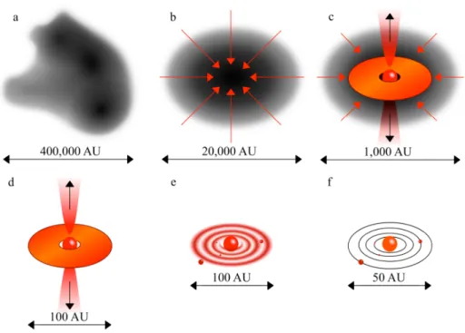
Figure 1.1:Schematic depiction of star formation: from GMCs to stars with planetary systems. Taken fromBraiding (2011).
has an impact on the structure of eventually forming planetary systems.
1.1 Associations and stellar clusters
Observations found that the majority of stars (70
−90%) form in stellar groups with
>100 stars (Lada & Lada, 2003). However, most of these groups in the solar neighbourhood seem to dissolve with time, as their birthrate is much larger than the observed number of groups would suggest. On the other hand, open clusters like for example Praesepe (Beehive Cluster, M44) or Hyades are 790
±60 Myr and 750
±100 Myr old, respectively, (Brandt &
Huang, 2015b,a) and still bound.
A distinction between the precursors of solar neighbourhood clusters and of clusters like Praesepe and Hyades can be made when looking at their formation and dynamical evolution.
1.1.1 Star formation in associations and clusters
Stellar clusters form from
Giant Molecular Clouds (GMCs)consisting of gas and dust with masses of 10
2−10
6M
, temperatures of 10
−20 K, and sizes of 10
−100 pc (Fig.
1.1a).Typically, the density in GMCs is low, between 20 M
pc
−2and of the order of 100 M
pc
−2(Elmegreen, 1985, 1993; Larson, 2003), so gravitational instabilities are necessary to trig-
1.1 Associations and stellar clusters
ger star formation (Fig.
1.1b). The GMCs may also have filamentary or clumpy structures(Williams et al., 2000), which – if they are massive and large enough – may form stellar groups. The minimum mass needed to get gravitational instabilities, and thus trigger star formation, is the
Jeans massMJ:
MJ
=
π6
c3s
G2/3ρ1/2,
(1.1)
where
csis the isothermal sound speed,
Gthe gravitational constant, and
ρthe density (see also Binney & Tremaine, 1987).
The collapsing gas forms
protostars, which are surrounded by a dust envelope fromwhich they accrete material (Dunham et al., 2014). Their temperature is too low to trigger hydrogen burning and radiation emitted from such stars usually stems from the accreted envelope, not from the core directly (1.1c). At first, the energy produced through the gravitational collapse can directly be transported away from the protostar’s surface by infra-red radiation. As more material is accreted, the system becomes opaque and the radiation cannot penetrate the dust envelope. Therefore, the core temperature increases further and the resulting pressure counteracts the gravitational in-fall of material (Larson, 1969). Eventually, the protostar blows away the remaining envelope, becoming optically visible and developing into a
pre-main-sequence star(PMS star, Fig.
1.1d). The core furthercontracts until the
hydrogen burningsets in once a temperature of 10
7K is reached. A balance between gravitational collapse and pressure from nucleosynthesis stabilises the core, yielding a
main-sequence star (MS star). The mass distribution of the newly formed starswithin a stellar group is usually described by a so-called
initial mass function (IMF), (cf.for example IMFs by Salpeter, 1955; Kroupa, 2002). For an overview of star formation and the involved processes, see for example Larson (2003); McKee & Ostriker (2007); Dunham et al. (2014) and Scilla (2016).
During protostar formation, a circumstellar disc forms around them due to angular mo- mentum conservation (Fig.
1.1c, see e.g.Cassen & Moosman (1981)). When the protostar turns into a PMS star, the disc can already show signs of structures, like spiral arms (Fig.
1.1e). If the protoplanetary disc is massive enough, a planetary system might formaround the star (Fig.
1.1f).During this process, even though up to several tens of thousands of stars can form together in a stellar cluster, only a portion of the gas of the GMC is transformed into stars.
This portion is quantified by the
star-formation efficiency(SFE):
SF E
=
MstarsMstars
+
Mgas,
(1.2)
where
Mstarsis the total stellar mass of the cluster and
Mgasthe mass of the left-over gas at the end of the star formation process.
With time, gas which is not already transformed into stars is driven outwards by a number of processes, for example, bipolar stellar outflows (Matzner & McKee, 2000), stellar winds of the most massive stars, or super-nova explosions (Zwicky, 1953; Pelupessy & Portegies Zwart, 2012).
The duration of this gas expulsion and the SFE mainly determine whether a group of stars disperses or remains bound (see e.g. Lada et al., 1984; Adams, 2000). Short-lived groups are referred to as
associations, whereas long-lived stellar systems are calledstellar clusters.It is important to note that there is no consistent nomenclature within the community, for example the term cluster might be used for all stellar aggregates, whose density is much higher than that of the stellar field, even if they are not necessarily bound in the long term (e.g. Fall & Chandar, 2012; Craig & Krumholz, 2013). In this thesis, as well as in the publications attached, the nomenclature
associationsfor short-lived and
clustersfor long-lived stellar groups will be used.
Figure
1.2shows the observed density and radius of a number of young and massive (> 10
3M
) associations (bottom) and clusters (top). The association/cluster ages are colour coded: very young systems are shown in red, systems between 4
−10 Myr in green, and older systems (> 10 Myr) in blue. It is evident, that the sizes and masses of clusters and associations evolve along two separate, well defined time tracks (Pfalzner & Kaczmarek, 2013b).
1The distinction of two types of stellar groups is not only visible in the Milky Way, also extragalactic clusters in the local group show this bimodal development (Da Costa et al., 2009).
It is important to note that there are studies claiming that the ”gap” in the half-mass radius mass plane between open clusters in the Milky Way and old globular clusters is filled by young, massive clusters like the Orion Nebula Cluster (ONC) (Portegies Zwart et al., 2010). However, it is questionable if systems like, for example, the ONC are massive enough to evolve into old, open or globular clusters. Currently it is unknown why stellar groups appear as either associations or clusters. Studies of globular clusters in the outer halo of the Galaxy indicate that the cluster formation process yields a bimodal distribution (Elmegreen, 2008; Baumgardt et al., 2010).
The two cluster types represent very distinct (birth) environments of protoplanetary discs and planetary systems, therefore, their properties and evolution are discussed in more detail in the following section.
1Note thatPfalzner(2009) uses the termleaky clusterfor associations andstarburst cluster for clusters.
1.1 Associations and stellar clusters
1 10
Cluster radius [pc]
0.01 1 100 10000 1e+06
Cluster density [M sunpc-3 ]
15000 Msunpc-3/R4 5000 Msunpc-3/R3
> 10 Myr 4Myr < age < 10Myr
< 4Myr
Galactic center cluster RSGC2
RSGC1
I Lac Upper Cen Lup Lower Cen Crux Ori Ia chi Per
h Per
U Sco Ori Ic Westerlund 1
Quintuplet
Ori Ib IC 1805NGC 7380 NGC 2244
NGC 6611 Cyg OB2 Arches
NGC 3606
Westerlund 2
DBS2003 Trumpler
CLUSTERS
ASSOCIATIONS
Figure 1.2:Observed densities and radii for clusters (top) and associations (bottom). The age of the systems is shown by colour: very young (<4 Myr) in red, 4−10 Myr in green, and old (>10 Myr) blue. Taken fromPfalzner(2009). The labels for cluster types were changed according to nomenclature used in this work.
1.1.2 Associations
Observations found that, in the solar neighbourhood, most associations disperse rather quickly (< 10 Myr) and their members become part of the
field star population(Lada &
Lada, 2003; Porras et al., 2003). Lamers & Gieles (2008) compared the star-formation rate in the solar neighbourhood and the surface density of open clusters – including effects like stellar evolution, tidal stripping, perturbations by spiral arms, and encounters with other GMCs – and estimated an
infant mortality, that is the dispersion of very young systems,of 50
−95%.
This high infant mortality cannot be explained by two-body dispersion of the clusters alone. Two-body relaxation becomes important after a timespan of
ttbr= 10N ln (N )
∗tcross, where
Nis the number of stars,
tcross=
R/Vthe crossing time,
Rthe cluster radius, and
Vthe average velocity (Binney & Tremaine, 1987). Even for a cluster with 1 000 stars, this yields
ttbr= 10
−100 Myr, which cannot account for the short dispersion timescale of
<
10 Myr found by observations (Krumholz et al., 2014).
One theory which can explain the fast dispersal is that these associations already formed
from gravitationally unbound GMCs (e.g. Clark et al., 2005). However, this kind of simu-
lations did not include stellar feedback, such that even unbound GMCs might form bound
stellar clusters (Krumholz et al., 2014).
Gas expulsion
Another explanation for the short lifetimes of associations in the solar neighbourhood is the effect of gas expulsion due to stellar feedback. Most of them have a rather low SFE of 30% at most (Lada & Lada, 2003), so when the remaining gas is expelled at the end of the star formation process, they lose 70% of their mass. As a result, they expand quickly and most – if not all – stars become unbound (Baumgardt & Kroupa, 2007).
Gas expulsion and its effect on associations and stellar clusters has been studied thor- oughly in the past, focussing on the conditions under which a bound remnant survives the gas expulsion (Tutukov, 1978; Hills, 1980; Lada et al., 1984; Goodwin, 1997a,b; Kroupa et al., 1999; Adams, 2000; Geyer & Burkert, 2001; Kroupa et al., 2001; Boily & Kroupa, 2003a,b; Fellhauer & Kroupa, 2005; Bastian & Goodwin, 2006; Baumgardt & Kroupa, 2007;
Goodwin, 2009; L¨ ughausen et al., 2012; Pfalzner & Kaczmarek, 2013a,b).
Figure
1.3shows the percentage of bound mass as a function of the SFE for associations (”loose massive clusters”) and star clusters (”compact massive clusters”). The higher the SFE, the more mass in associations remains bound. In the more compact clusters, however, the bound mass does not exceed
≈82% in the simulated models. They are less susceptible to gas expulsion, but they continuously lose stars due to gravitational interactions between the cluster members (Pfalzner & Kaczmarek, 2013b).
Star formation within a clump is not homogeneous. Observations found that the local surface density of
young stellar objects (YSOs)depends on the local column density of the gas within the cloud (Gutermuth et al., 2011). This local dependence can be described by the
star formation efficiency per free-fall time f f(Krumholz & McKee, 2005; Parmentier
& Pfalzner, 2013). Even systems with a low overall SFE of 10% can thus form systems which leave a bound remnant after gas expulsion, because the SFE in the system centre is higher. In summary, recent studies found that an SFE between 10% and 35% is needed to form a bound association.
However, the bound fraction is not only a function of the SFE, but also of the timescale on which the gas is expelled. The
gas-expulsion timescaleis considered to be of the order of, or smaller than, the
dynamical timescaleof the association/cluster, which describes the time a typical star needs to cross the system:
tdyn
=
GMcl r3hm
−1/2
,
(1.3)
where
Gis the gravitational constant,
Mclis the total association/cluster mass, and
rhmthe half-mass radius (Geyer & Burkert, 2001; Melioli & de Gouveia dal Pino, 2006; Porte-
gies Zwart et al., 2010). Typical dynamical timescales of associations can be between a few
Myr up to several tens of Myr, whereas for clusters they are of the order of 1 Myr or less.
1.1 Associations and stellar clusters
0 20 40 60 80 100
star formation efficiency(%) 0
20 40 60 80 100
percentage of bound mass
low density cluster loose massive cluster compact massive clusters
Figure 1.3:Simulated percentage of bound mass as a function of the SFE after a simulation time of 20 Myr for low-density clusters (dashed line, triangles), association (drawn line, circles), and clusters (dotted line, diamonds); taken fromPfalzner & Kaczmarek(2013a). Note that associations are called loose clusters and clusters are called massive clusters here.
A compilation can be found in (Portegies Zwart et al., 2010).
If the gas expulsion is slow, i.e. adiabatically, even associations with a relatively low SFE can remain bound, because they have enough time to adjust to the mass loss. On the other hand, if the expulsion happens fast, a high SFE is required to yield a bound remnant.
In addition, the more substructure an association/a cluster shows, the more probable it is to remain bound (see e.g. Smith et al., 2011). It is important to note that even if a remnant remains bound, its surface density might be so low that it would not be detected by observations which are based on searches for stellar surface densities (Pfalzner et al., 2015b).
Another key parameter for association/cluster survivability is the virial ratio
Q=
−T /U,which is the ratio between kinetic and potential energy (see also Goodwin, 2009). An asso- ciation or a cluster in virial equilibrium (Q = 0.5) is dynamically stable, whereas so-called
hotsystems (Q > 0.5) are bound less strongly and expand; in
coldsystems (Q < 0.5) the gravitational energy dominates and the systems contract. As a result, hot systems are more prone to destruction compared to systems which are in virial equilibrium or cold (see e.g. Goodwin, 2009). After gas expulsion, the system is out of virial equilibrium, which it regains within a few crossing times, if a bound remnant remains.
In summary, four parameters determine whether an association/a cluster is destroyed
or a bound cluster remains: the SFE, the duration of the gas expulsion itself, the stellar
distribution within the association/cluster, and the virial ratio Q.
The Orion Nebula Cluster
One of the most studied associations is the Orion Nebula Cluster, because it is the closest dense stellar group in which stars are still formed. It contains about 4 000 stars, is roughly 1 Myr old and has a half-mass radius of about 1 pc (Hillenbrand & Hartmann, 1998). It still contains some of its gas and is therefore used as a model for young, massive, embedded clusters in many numerical studies concerning protoplanetary discs and their evolution (see e.g. Scally & Clarke, 2001; Olczak et al., 2006; Pfalzner & Olczak, 2007; Steinhausen et al., 2012; Portegies Zwart, 2016).
Observations of today’s ONC suggest an approximately isothermal density profile in the outer parts of the cluster (McCaughrean & Stauffer, 1994; Hillenbrand & Hartmann, 1998) and a flatter profile in the core (Scally et al., 2005). Olczak et al. (2010) provide a three- dimensional density distribution which, after 1 Myr of evolution, yields the current density distribution of the ONC:
ρ0
(r) =
ρ0
(r/R
0.2)
−2.3, r∈(0, R
0.2]
ρ0(r/R
0.2)
−2.0, r∈(R
0.2, R]0, r
∈(R,
∞],(1.4)
where
ρ0= 3.1
×10
3stars pc
−3is the density,
R0.2= 0.2 pc the core radius, and
R= 2.5 pc the cluster radius.
Associations in general cover a wide density range, for example the ones presented in Fig- ure
1.2have densities between 0.07
−40 M
pc
−3(Pfalzner, 2009, and references therein).
The initial conditions in the simulations discussed in the papers included are chosen in such a way as to cover this wide range of densities. They all have the same density profile and, as such, can be regarded density-scaled versions of the ONC, meaning that the half-mass radius and the density distribution are the same as for the ONC. However, the number of stars was varied: models with 1 000, 2 000, 4 000 (ONC model), 8 000, 16 000, and 32 000 stars were simulated.
1.1.3 Compact clusters
In contrast to associations, young, massive stellar clusters are much denser and eventually develop into open clusters, which can become several hundreds of millions of years old.
Clusters – also called compact clusters or starburst clusters – are preferably located in the Galactic centre and in the spiral arms. Estimates predict that only about 10% of all stars in the Milky Way are born in such long-lived clusters (Schweizer, 2006).
The major difference in the formation process between clusters and associations are the
1.2 Protoplanetary discs and extrasolar planets
much higher SFE (Bastian, 2011; Pfalzner & Kaczmarek, 2013a,b), and the smaller half- mass radius at the end of star formation (Stolte et al., 2010). Observations of young, massive clusters find rather low velocity dispersions in the systems, making it likely that they are in or close to virial equilibrium (see e.g. Mengel & Tacconi-Garman, 2007; Clark- son et al., 2012; H´ enault-Brunet et al., 2012). As the observed clusters are still young, this could indicate that their SFE was high. Comparing observations to numerical simulations of clusters, Pfalzner & Kaczmarek (2013b) found that the evolution of clusters with an SFE of 60
−70% is in accordance with the observed increase in cluster size during the first 20 Myr. This high SFE renders them less prone to disruption due to gas expulsion.
However, clusters lose mass and expand as well, see Figure
1.3(dotted line, diamonds).
The reason for this are stellar interactions, which lead to ejections of stars from the clusters and, consequently, to expansion (Pfalzner & Kaczmarek, 2013b).
Two of the most well observed young, massive clusters are Arches and Westerlund 2.
Both are between 1.5
−2.5 Myr old, have a mass of the order of 10
4M
and densities of 4
·10
5M
pc
−3and 5
·10
3M
pc
−3, respectively (Figer, 2008, and references therein).
They will most probably develop into open clusters like the Hyades or Praesepe (790
±60 Myr and 750
±100 Myr, respectively, see Brandt & Huang, 2015b,a).
Arches was taken as a model for the simulations of clusters in this theses, assuming an initial half-mass radius of 0.2 pc (core radius of current Arches, see Stolte et al., 2010) and a stellar population of 32 000 stars, analogue to the most massive association and in accordance with Arches’ current mass (Figer, 2008, and references therein). To date, no gas-embedded precursor of clusters has been detected, thus, the embedded phase is most probably very short, as is the gas expulsion itself. Therefore, two different types of cluster simulations were performed. The first type was embedded for 1 Myr, which is an upper limit for the embedded timescale. In the second type of clusters, the gas was expelled at the beginning of the simulations (t
emb= 0 Myr), mimicking a very short embedded time of
temb1 Myr.
1.2 Protoplanetary discs and extrasolar planets
Protoplanetary discs form as a consequence of angular-momentum conservation around most – if not all – stars. The launch of the
Hubble Space Telescope (HST)made it possible to directly detect discs, for example, around young stars in the ONC (O’dell et al., 1993).
Since then, a large number of protoplanetary discs around field stars, as well as around
association and cluster members has been found. Together with theoretical models and
Figure 1.4:Schematic depiction of a protoplanetary disc. The physical grain-growth processes are depicted on the left of the plot. On the bottom right, different telescopes are listed: theAtacama Large Millimeter/sub- millimeter Array (ALMA), theVery Large Telescope Interferometer (VLTI)with the Multi Aperture Mid-Infrared Spectroscopic Experiment (MATISSE), theEuropean Extremely Large Telescope (EELT), and theJames Webb Space Telescope (JWST)with theMid-Infrared Instrument (MIRI). The colours depict the areas within the disc which they oberve with their given rage of wavelengths. The axis shows the logarithmic radial distance from the central star in AU. Taken fromTesti et al.(2014).
simulations, the evolution of discs and eventually forming planetary systems has been studied thoroughly.
Here, only a brief overview of disc evolution, dust growth, and planet formation will be given. For a comprehensive review see, for example, Testi et al. (2014).
At birth, a protoplanetary disc consists of gas and dust from the GMC. The dust par- ticles are micrometer-sized and thus coupled to the gas. Larger dust particles sink to the mid-plane of the disc (vertical settling) and are transported inwards (radial drift ), whereas small particles are mixed vertically by turbulences and are transported outwards. Drag forces (Whipple, 1972; Weidenschilling, 1977), radial drift (Whipple, 1972; Adachi et al., 1976; Weidenschilling, 1977), dust trapping, and radial mixing lead to collisions of dust particles and therefore grain growth, as long as their relative velocities are low. Addition- ally, condensation of gaseous material or the sublimation of solids can form small particles, but these effects are less important for larger dust grains (see Testi et al., 2014).
Due to the partial sorting of the particles by size within the disc, its different areas can
be observed with specific wavelengths. This is important to keep in mind when it comes
to the measurement of the disc size, as the observational techniques may otherwise limit
or bias the resulting size. Figure
1.4depicts a simplified protoplanetary and its internal
1.2 Protoplanetary discs and extrasolar planets
structure (right). The areas within the disc are colour coded, the corresponding wavelengths and telescopes, with which the different areas can be observed, are presented below. The grain-growth mechanisms are shown on the left hand side of the picture.
1.2.1 Protoplanetary-disc lifetimes and destruction processes
If the discs are massive and dense enough, planets or planetary systems might form. There- fore, the lifetime of protoplanetary discs constrains the formation and evolution time of planets significantly. It is not straightforward to determine the age of young stars and their protoplanetary disc. Especially around field stars this is rather difficult and prone to significant errors. The age of stellar clusters and associations can be constrained to a certain degree with the help of their
Hertzsprung-Russel diagram (HRD), which depicts theluminosity and the effective temperature of the cluster members. When stars have turned most of their hydrogen in the core to Helium, they turn into red giants, and leave the main sequence in the HRD. This point is called the
Main-Sequence turn-offand quantifies the cluster age, assuming that all stars formed at the same time. Multiple Main-Sequence turn-offs can be either a sign of a stellar age spread within the cluster or of cluster-rotation (see Yang et al., 2013, and references therein). Therefore, it is preferable to observe discs in associations or clusters to constrain the formation, evolution, and (possibly) destruction timescales more accurately. However, a dense environment leads to observational difficul- ties, for example, due to the high luminosity in the centre.
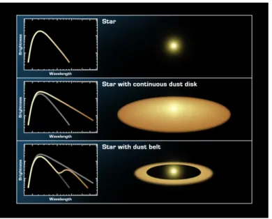
Figure 1.5:SED of a star without a disc (black body, top), of a star with a smooth dusty disc (mid), and of a star with a dust belt (disc with gap, bottom). Credit: NASA/JPL-Caltech/T. Pyle (SSC), http:
//www.spitzer.caltech.edu/images/2632-sig05-026-The-Invisible-Disk.
A disc surrounding a star can not only be discovered directly, but also indirectly through the infra-red excess in the stellar
spectral energy distribution (SED). If a disc is present,the SED shows characteristic deviations (Figure
1.5mid and bottom) from the one of a black body (Figure
1.5top).
If the membership of an association/a cluster is well determined, the
disc fraction, i.e.the fraction of stars in the stellar group, which is surrounded by a protoplanetary disc, can be obtained. With the help of the disc fraction of many associations/clusters and the systems’ age, the timescales of disc formation and of the influence of external effects by the environment can be constrained.
The disc fraction has been determined by observations in a variety of associations and clusters, and seems to decline with association/cluster age, see Figure
1.6.Haisch et al.
(2001) concluded from their investigation of clusters (black points) that almost all stars lose their disc within the first 5 Myr. Taking more clusters into account, Mamajek (2009) revised the linear fit by Haisch et al. (2001) by fitting an exponential function of the disc fraction to the data and found a half-life time of 2
−3 Myr.
However, recently, there have been cautious remarks concerning these disc lifetimes (Pfalzner et al., 2014), as selection effects might bias the data above. Firstly, the de- picted clusters with ages of
>3 Myr (after gas expulsion) are rather large and massive.
Younger systems, which are still forming stars, will not necessarily evolve in the same way, because they do not contain enough gas to reach such masses. Thus, the sample of clusters is inhomogeneous.
Secondly, the systems lose stellar members due to gas expulsion and stellar interactions.
Especially associations respond very strongly to gas expulsion, as a result, they usually cover several tens of parsecs in radius. However, observations focus on the inner few parsecs, where the stellar density is highest. This means that the plot depicts only the stars which still reside within a few parsecs from core after gas expulsion took place, which might not be representative for the cluster as a whole.
Thirdly, clusters as well as associations expand, which means that the stars which ini- tially resided in the innermost, densest part of the system now cover the inner few parsecs.
Observations therefore pick out discs which are most likely already influenced or destroyed by fly-bys, external photoevaporation, and other effects.
Summarising, the data in the above mentioned work depicts the discs around stars 1. in massive clusters,
2. which reside within a few parsecs of the cluster after gas expulsion,
3. and originated from the very dense system centre.
1.2 Protoplanetary discs and extrasolar planets
Figure 1.6:Disc fraction as a function of system age. Open symbols represent embedded associations/clusters, filled symbols associations/clusters after gas expulsion. The red symbols depict very low-density associations.
The purple symbols indicate associations where the disc fraction was observed outside the cluster core.
Taken from Pfalzner et al.(2014), based onHaisch et al.(2001) (linear fit, dashed), Mamajek(2009) (exponential fit, solid), and values fromFang et al.(2013) (low-density associations, red).
Therefore, according to these new findings, the lifetimes of discs in very low-density associations, for example, are much longer than predicted before (red squares in Fig.
1.6,see also Pfalzner et al. (2014)).
This poses a crucial question:
Are protoplanetary discs and planetary systems in associations and clusters similar, or is there a systematic influence of the environment on their shape?To investigate this, the different processes involved in protoplanetary disc destruction or manipulation will be discussed in more detail in the following.
Internal disc-dispersal mechanisms
There are a number of processes which can alter or completely destroy a protoplanetary disc, for example viscous torques (Shu et al., 1987), turbulent effects (Klahr & Bodenheimer, 2003), magnetic fields (Balbus & Hawley, 2002), and viscous accretion (Lynden-Bell &
Pringle, 1974).
Currently, one favoured disc-dispersal process is
internal photoevaporation, meaning thatstrong stellar winds of the disc-hosting star can heat up and/or blow away material from the
disc (Hollenbach et al., 1994). The strength of the internal photoevaporation is affected by
the radiative transfer within the disc, hydrodynamics, and thermodynamics. In addition,
optically thick discs are affected differently than optically thin discs (Alexander et al.,
2014).
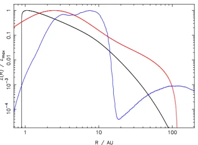
Figure 1.7:Normalised mass-loss profile, i.e. the mass loss at radiusR, ˙Σ(R), devided by the maximum mass loss Σ˙max, due to photoevaporation by EUV radiation (black,Font et al.(2004)), X-rays (red,Owen et al.
(2012)), and FUV radiation (blue,Gorti et al.(2009)), as a function of the disc radius R. Taken from Alexander et al.(2014).
To date, it is computationally not possible to include all the above effects in an all- encompassing simulation, therefore, separate numerical simulations are performed to study the effects and the strength of the photoevaporation. One way of classifying different wave- length regimes in the simulations is to distinguish between
far-ultravioletradiation (FUV, 6-13.6 eV),
extreme ultravioletradiation (EUV, 13.6-100 eV), and
X-rays(100 eV-10 keV), see Alexander et al. (2014). 13.6 eV is the ionization energy of atomic hydrogen. Below this energy, mainly neutral dissociation of molecules takes place. The different types of radiation are most effective in different parts of the disc. They will be discussed in more detail the following, an overview of the areas where they are most effective is given in Figure
1.7.EUV radiation ionises hydrogen atoms in the disc, such that an ionised atmosphere forms. Close to the star, the material is still bound, but beyond the critical radius
Rc,EU V= 1.8
·(M
star/1 M) AU it becomes unbound in form of ionised wind (Alexan- der et al., 2014).
X-rays are capable of inner-shell ionising heavy elements, for example oxygen, carbon, and iron. The resulting photoelectrons heat up the hydrogen atoms/molecules, creating a smooth transition from a very hot corona close to the star, to an ionised atmosphere, and down to a cold disc. The mass loss due to X-rays is larger than the one caused by EUV (Owen et al., 2012).
Finally, in photoevaporation simulations, FUV radiation is usually assumed to be non-
ionising and
H2dissociating. It is mostly absorbed by dust grains and then re-emitted
1.2 Protoplanetary discs and extrasolar planets
as IR continuum. In contrast to EUV radiation and X-rays, FUV radiation is capable of depleting the disc mass at large radii (≥ 100 AU, see also Gorti & Hollenbach (2009)).
However, its effectiveness strongly depends on the incident flux and the density of the disc.
There is still much ongoing work in order to constrain the heating/cooling rates in the discs and thus the importance of FUV radiation.
External disc dispersal mechanisms
In addition to internal photoevaporation, massive stars in the vicinity of a disc-hosting star influence the outer parts of the disc (external photoevaporation, see e.g. Johnstone et al. (1998); St¨ orzer & Hollenbach (1999); Scally & Clarke (2001); Clarke et al. (2001);
Matsuyama et al. (2003); Johnstone et al. (2004); Alexander et al. (2005, 2006); Ercolano et al. (2008); Drake et al. (2009); Gorti & Hollenbach (2009); Winter et al. (2018b)).
The timescales on which external photoevaporation can destroy discs are still under discussion. Simulation results vary between
tphoto ≈0.1 Myr up to
≈10 Myr (numerical simulations by Scally & Clarke, 2001; Gorti & Hollenbach, 2009; Adams et al., 2006; Winter et al., 2018b). A recent study argues that photoevaporation within a cluster with a number density of
nc ≈10
4(comparable to the models presented above) is the main mechanism shaping and destroying protoplanetary discs within 3 Myr (Winter et al., 2018b). They estimate that even the gas in the clusters is not capable of preventing disc destruction due to photoevaporation. However, they did not model the gas explicitly, instead, they took a Monte Carlo approach to obtain the fly-by history of the stars and the disc sizes after fly-bys. The stars remain in a ”fixed stellar environment” for the whole simulation time, exposed to constant FUV radiation with
G0= 3000 (Winter et al., 2018b). However, associations react strongly to gas expulsion after 2 Myr and stars move outwards, away from each other and the most massive association members. Therefore, the effect might be overestimated for those discs. If a disc-hosting star resides far away from the most massive cluster members, or becomes unbound as a result of gas expulsion, its disc will most probably not be influenced significantly by external photoevaporation. Discs which reside sufficiently close to or pass by massive stars are most probably destroyed by either mechanism, fly-bys or photoevaporation. For a detailed overview of the theoretical basis of internal and external photoevaporation and their effects, see e.g. Alexander et al. (2014).
Stellar interactions
The external process which is investigated in detail in this work is
stellar interactions.2Associations and stellar clusters are highly dynamical environments and stellar fly-bys can
2In the publications attached, these interactions are calledencounters orfly-bys.
Figure 1.8:Pictures of the protoplanetary discs around HL Tauri (left) and TW Hydrae (right) taken with the Atacama Large Millimeter/submillimeter Array (ALMA). Credit left: ALMA (ESO/NAOJ/NRAO), http://www.eso.org/public/images/eso1436a/. Credit right: S. Andrews (Harvard-Smithsonian CfA);
B. Saxton (NRAO/AUI/NSF); ALMA (ESO/NAOJ/NRAO), http://www.eso.org/public/images/
eso1611a/.
change the angular momentum, the mass, and the size of the discs (see e.g. Clarke &
Pringle, 1993; Hall, 1997; Scally & Clarke, 2001; Olczak et al., 2006; Pfalzner et al., 2006;
Pfalzner & Olczak, 2007; Olczak et al., 2010; de Juan Ovelar et al., 2012; Breslau et al., 2014; Rosotti et al., 2014; Steinhausen & Pfalzner, 2014; Vincke et al., 2015; Portegies Zwart, 2016; Vincke & Pfalzner, 2016; Breslau et al., 2017; Winter et al., 2018a).
The size is most sensitive to changes due to stellar interactions, because fly-bys can push material inwards without removing it, thus shrinking the disc without changing its mass (Hall, 1997; Rosotti et al., 2014; Vincke et al., 2015). Together with the disc mass, the disc size pre-defines the position and mass of eventually forming planets.
There are two main methods of disc observation: direct and indirect detection. Con- nected with this, there are also two ways of determining the sizes of protoplanetary disc sizes. Two very famous examples of direct detection are shown in Fig.
1.8, namely thediscs HL Tauri and TW Hydrae, which show signs of structure (rings). The size of such discs is usually determined by taking the outer luminosity drop as the disc radius (O’dell, 1998; Vicente & Alves, 2005). Large, luminous discs in the vicinity of the Sun are the best candidates for direct detection, as they are bright enough to be around their host star.
Smaller discs which are less luminous and/or too far away can be detected indirectly by analysing the SED of a star, looking for infra-red access. The disc size is then assumed to be the truncation radius of the disc (see e.g. Andrews & Williams, 2007).
A number of protoplanetary discs have been found in associations like, for example, Tau-
rus, the ONC, and Ophiuchus (McCaughrean & O’dell, 1996; Vicente & Alves, 2005; An-
1.2 Protoplanetary discs and extrasolar planets
drews & Williams, 2007; Eisner et al., 2008; Andrews et al., 2009, 2010; Brinch & Jørgensen, 2013; Harsono et al., 2014). Their radii range from about 10 AU up to
≈500 AU in the ONC (McCaughrean & O’dell, 1996) to up to 700 AU in Ophiuchus (Andrews & Williams, 2007). However, even in these low-stellar-density environments, it is questionable whether the discs are pristine or already shaped by, for example, fly-bys of other association mem- bers.
To study the effect of fly-bys on protoplanetary discs in more detail, a variety of theo- retical models and numerical simulations have been developed and performed in the last decades. Most of them have modelled isolated star-disc fly-bys, where one star – surrounded by a disc – is passed by another star without a disc. They found a very simple connection between the disc size after the fly-by and the periastron distance of the passing star: the disc is truncated to 1/2 (Clarke & Owen, 2015) or 1/3 (Hall et al., 1996; Kobayashi &
Ida, 2001) of the fly-by’s periastron distance (e.g. Adams et al., 2006; Brasser et al., 2006;
Adams, 2010; Malmberg et al., 2011; Jim´ enez-Torres et al., 2011; Pfalzner, 2013). However, these disc-size limits were obtained only considering
equal-mass fly-bys, meaning that thedisc-hosting star and the perturbing star have the same mass. However, the stellar masses in associations and clusters cover a broad parameter space, therefore, the mass ratio be- tween two interacting stars is, in most cases, not unity.
In principle, it would be preferable not to model such star-disc interactions in isolation, but to accurately model protoplanetary discs within an association or a stellar cluster, and then to determine their size after each stellar fly-by. Rosotti et al. (2014) performed such simulations, combining
smooth-particle hydrodynamics (SPH)simulations of discs and NBody simulations of an association of 100 equal-mass stars, and evolving the association for 0.5 Myr. They found that discs can indeed be strongly influenced by stellar fly-bys.
The difficulty with such combined simulations is that they are computationally very costly.
Stellar clusters, which are much more massive and much denser than the association studied by Rosotti et al. (2014), can therefore not be studied with a realistic initial mass function (see Sect.
1.4.1) with these kinds of simulations.Therefore, a two-step approach is taken here, separating the simulation of young, massive associations/clusters with NBody from the disc simulations, which are described in more detail in Sect.
1.4.Breslau et al. (2014) defined a disc-size limit which mimics the disc sizes as they would
be found by observations: they took the steepest point in the disc’s density distribution as
the outer disc rim. With this criterion, they performed an extensive parameter study of star-disc fly-bys, with different periastron distances and stellar-mass ratios. They found a simple dependence of the final disc size
rdiscon these parameters:
rdisc
=
0.28
·rperi·m−0.3212 ,if
rdisc < rprevious rprevious,if
rdisc ≥rprevious,,
(1.5)
where
m12=
m2/m1is the mass ratio between the disc-hosting star (m
1) and the per- turber (m
2),
rperithe periastron distance in AU, and
rpreviousis the disc size previous to the fly-by in AU. This equation is valid for all types of mass ratios typically found in clusters, but covers only coplanar, prograde, parabolic fly-bys. The disc was assumed to be flat, and to consist of mass-less tracer particles, that means that no viscosity or self-gravity was included. For a detailed description of the simulation set-up, the approximations made, and their influence on the results, see Breslau et al. (2014) and Vincke et al. (2015).
On the basis of this work, Bhandare et al. (2016) extended the parameter study to include
randomly orientatedfly-bys, meaning that the perturber orbit and the disc are not necessarily in the same plane. In extreme cases, the fly-by could also be retrograde.
According to their results, the disc size after a fly-by – averaged over all inclinations ranging from 0-180 degrees – only depends on
rperiand
m12:
3rdisc
= 1.6
·r0.72peri·m−0.212 .(1.6) This fit-formula focusses on penetrating (r
peri ≤ rprevious) or very close fly-bys. The largest periastron distances included are 5 times the initial disc size
rinit. For more details and the non-averaged data, see Bhandare et al. (2016).
1.2.2 Extrasolar planets
Under specific conditions, planets or planetary systems can form from protoplanetary discs on timescales of less than one to several tens of millions of years (cf. e.g. Alibert et al., 2005; Pfalzner et al., 2015a). The first confirmed extrasolar planet – or short
exoplanet– around a pulsar was found by observations in 1992 (Wolszczan & Frail, 1992), the first one around a main sequence star three years later (Mayor & Queloz, 1995). Since then, observations have found a little more than 3 700 exoplanets
4, see Figure
1.9.3An open access data base of their results for the whole parameter space covered (periastron distance, mass ratio, inclination, and angle of periastron) as well as a tool to easily plot disc/particle properties after fly-bys can be found athttp://www3.mpifr-bonn.mpg.de/encounter-properties/.
4Value taken fromhttps://exoplanets.nasa.gov/newworldsatlas/on 22 May, 2018.
1.2 Protoplanetary discs and extrasolar planets
1990 1995 2000 2005 2010 2015
1200
1000
800
600
400
200
0
First Publication Date
Distribution
exoplanets.org | 5/22/2018
Figure 1.9:Number of exoplanets found since 1990. The plot was produced onhttp://exoplanet.eu/(Han et al., 2014) on 22 May, 2018.
A stellar fly-by can not only shape a protoplanetary disc, but also force an already formed planet on a different orbit. In extreme cases, planets can even become unbound.
If more than one planet is present in the system after the fly-by, long-term instabilities can be triggered, leading to planet-planet scattering (Davies et al., 2014). The timescale of isolated star-disc fly-bys which influence the disc is, depending on the mass ratio and periastron distance, of the order of 10
3−10
4yr.
Detection and statistics
There is a variety of detection mechanisms for exoplanets, for example
direct imaging, transit photometry, astrometry, radial velocity (RV) measurements, several time-variation measurements, andgravitational microlensing. Each of these has biases according to whichtype of planets it can detect. As a result, the planets and planetary systems detected might be biased towards close-in, massive, large planets, because most have been detected via transit photometry, followed by RV measurements and direct imaging.
So far, most exoplanets and exoplanetary systems have been detected around field stars.
Determining the age of such planets/planetary systems and their host stars is very difficult.
Without a clear restriction on a system’s age, conclusions about its evolutionary phase,
planet formation processes, and timescales are somewhat speculative. The advantage of
stellar clusters and associations is that their ages – and therefore the stellar ages – can be
determined well. However, it was speculated for a long time whether planetary systems
can exist at all in the very hostile environment of dense, long-lived clusters (e.g. Paulson
et al., 2004).
Table 1.1:Observed properties of planets in open clusters.
Cluster properties Planet properties References
Cluster
tclHost star
mpl apl epl[Myr] [ M
X] [AU]
NGC 4349 200 No. 127 19.8
a)2.38 0.19 (1)
Praesepe/M44 578
±12 Pr 0201 0.540
a)0.057 0 (2), (3), (4) Pr 0211 1.8a), b) 0.03
b)0.011
b)(4), (5)
7.79
a)5.5 0.71 (5)
K2-95 — 0.069
d)0.16 (6)
K2-100 — 0.029
d)0.24 (6)
K2-101 — 0.11
d)0.10 (6)
K2-102 — 0.083
d)0.10 (6)
K2-103 — 0.13
d)0.18 (6)
K2-104 — 0.025
d)0.18 (6)
Hyades 625
±50 Tau 7.6 1.93 0.151 (7), (8)
HD 285507 0.917
a)0.06
d)0.086 (9) LP 358-348 0.0047 0.075
d) <0.72 (10)
0.0365 0.132
d) <0.47 (10) 0.0145 0.162
d) <0.75 (10)
K2-25
<3 — 0.27 (11)
NGC 2423 750 No. 3 10.6
a)2.10 0.21 (1)
NGC 6811 1 000
±170 Kepler 66
≤0.06 0.1352 — (12), (13) Kepler 67
≤0.06 0.1171 — (13)
M 67 3 500
−4 000 YBP1194 0.34
a)0.07 0.24 (14), (15), (16) YBP1514 0.40
a)0.06
d)0.39 (16)
SAND364 1.54
a)0.53
d)0.35 (16) YBP401 0.46
a)0.05
d)0.15 (17), (18)
Notes: Column 1 indicates the cluster name and Col. 2 its age tcl; Col. 3 gives the name of the planet- hosting star,mpl the planet mass,apl its semi-major axis,eplits eccentricity, and Col. 7 the references.
References: (1)Lovis & Mayor(2007), (2) Delorme et al. (2011), (3) Kraus & Hillenbrand (2007), (4) Quinn et al. (2012), (5)Malavolta et al.(2016), (6) Mann et al.(2016b), (7) Perryman et al.(1998), (8) Sato et al. (2007), (9) Quinn et al. (2014), (10)Livingston et al. (2018), (11)Mann et al. (2016a), (12) Janes et al.(2013), (13)Meibom et al.(2013), (14)Sarajedini et al.(2009), (15)Richer et al.(1998), (16) Brucalassi et al.(2014), (17)Pietrinferni et al.(2004), (18)Brucalassi et al.(2016).
Comments: a) given asmpl∗sin(i), where i is the inclination between the orbital plane and the line of view;
b) combined planet properties from (4) and (5); c) note the large error in fitted period: P = 4 850+4560−1750 days; d) calculated from given orbital periods. Taken fromVincke & Pfalzner(2018).
1.3 The Solar System
The number of detected planets in clusters is still low, but to date, 23 exoplanets have been found in open clusters, among them even a planetary system in Praesepe (M44), see Table
1.1. Two planets orbit the star PR 0211, the inner one on a nearly circular orbit(e = 0.01) very close to the star with a semi-major axis of
apl= 0.03 AU, the outer planet, however, resides at
apl= 5.5 AU on a very eccentric orbit (e = 0.7). Such a system could have been shaped by a stellar fly-by with a probability of about 10% for a system being cut down to the size of PR 0211 (Pfalzner et al., 2018). In addition to the disc size, a fly-by can change the orbits of already formed planets at the outer rim of the system. They can be excited to eccentric orbits, while planets close to the star remain (almost) unperturbed (see Bhandare et al., 2016; Pfalzner et al., 2018).
It is expected that planetary systems in open clusters are much smaller than in associ- ations. Simulations suggest that, the denser an association or a cluster is, and the more substructure it has, the less probable it is that a planetary system survives (Zheng et al., 2015). However, the interaction rate in associations with 100
−1 000 stars was found to be low, such that most systems in such environments remain unperturbed (Adams et al., 2006).
The question is: does the environment leave an imprint on protoplanetary discs or already formed planetary systems though stellar fly-bys?
1.3 The Solar System
Investigating fly-bys in associations/clusters is not only interesting in terms of exoplanetary- system formation, but also when it comes to the formation of our own solar system. It is very probable that our Sun was – like 90% of all stars – born in an association or a cluster.
Therefore, it could have undergone a stellar fly-by by one or several siblings of the Sun, i.e.
stars which were born in the same environment.
1.3.1 Indications for early membership in an association or a stellar cluster There are several indications that the Sun might have indeed been part of an association or a stellar cluster, the strongest indicators are the following:
Outer edge
The surface density of the solar system drops steeply – by a factor of more than 1 000
(Morbidelli et al., 2003) – outside Neptune’s orbit at
≈30 AU. This so-called
outer edge cut-offimplies that the solar protoplanetary disc must have extended to at least this value
to enable planet formation. A stellar fly-by could be the culprit for the cut-off, stripping
most material outside 30 AU away, leaving a clear edge behind (Ida et al., 2000; Kobayashi
& Ida, 2001; Melita et al., 2002; Pfalzner et al., 2015a).
Highly eccentric Trans-Neptunian objects
In the Kuiper belt region, many objects on highly eccentric, inclined orbits can be found.
For most of them, the deviation from the planetary plane can be explained by interac- tions with the planets. However, there exists a group of so-called
Trans-Neptunian objects (TNOs)– with a very large pericentre and high eccentricity – whose orbits cannot be ex- plained by interactions with the planets alone (see e.g. Gladman et al., 2002). Examples for such extreme TNOs are Sedna (Brown et al., 2004), 2012 VP
113(Trujillo & Sheppard, 2014), 2014 UZ
224(Gerdes et al., 2017), 2004 VN
112Becker et al. (2007), and 2010 GB
174(Chen et al., 2013).
Culprits responsible for the TNOs’ unusual orbital parameters could be stellar fly-bys (see e.g. Brown et al., 2004; Kenyon & Bromley, 2004; Morbidelli & Levison, 2004; Rickman et al., 2004; Brasser et al., 2006; Dukes & Krumholz, 2012; Soares & Gomes, 2013; Brasser
& Schwamb, 2015) or perturbations caused by an additional planet (Brown et al., 2004;
Gomes et al., 2006; Soares & Gomes, 2013). This proposed
ninth planetin the outer solar system could be responsible for the large pericentres and high eccentricities of some TNOs (Batygin & Brown, 2016a). However, it is still under debate whether one planet alone can reproduce the observed simultaneous clustering in argument of pericentre, longitude of the ascending node, and longitude of perihelion of the TNOs (Shankman et al., 2017).
Abundances of short-lived radionuclides
The abundances of precursors of
short-lived radionuclides (SLRs), most prominently of60
Fe (t
1/2= 1.5 Myr) and
26Al (t
1/2= 1.7 Myr), found in
calcium-aluminium rich inclu- sions (CAIs)in chondritic meteorites (MacPherson et al., 1995) are thought to have been produced by supernova explosions. As such massive stars predominantly exist in rather massive stellar groups, it is probable that the protoplanetary solar system was part of a massive association or a stellar cluster (see e.g. Nicholson & Parker, 2017). A single super- nova very close (≤ 0.3 pc, Adams, 2000) to the Sun could have enriched the protoplanetary solar disc directly during its explosion (Chevalier, 2000; Busso et al., 2003; Ouellette et al., 2007). A progenitor of such a supernova has to have a stellar mass of
≈25 M
(Adams, 2000), and is thus most probable to form in a massive cluster. However, the details of the enrichment process(es) are still under debate.
Some studies argue that
60Fe does not necessarily has to have been injected by a super-
nova, and that typical molecular clouds already contain enough
60Fe – and possibly
26Al –
to explain today’s abundances in the solar system (Gounelle & Meibom, 2008; Gounelle
1.3 The Solar System
Table 1.2:Constraints on birth environment of the solar system.
Variable Value Limiting factor References N
>4 000 chemical composition Lee et al. (2008) N
<several 10
4radiation field Adams (2010)
ρC >10
3M
pc
−3Sedna orbit Brasser et al. (2006)
ρC <10
5M
pc
−3Sedna orbit Schwamb et al. (2010)
Notes: N is the number of stars in the system andρCthe cluster density. Taken fromPfalzner(2013).
et al., 2009). The abundance of
60Fe and
26Al in the early solar system could also be a hint of hierarchical star formation within an association/a cluster, with the Sun being a second- or third-generation star, and the disc being imprinted by the first and second generation stars (Gounelle & Meynet, 2012; Gritschneder et al., 2012; Gounelle, 2015).
Which of the scenarios – direct pollution or triggered star formation – is most probable is still a topic of debate, see e.g. Parker & Dale (2016). A detailed discussion of the different enrichment scenarios can be found in Sect.
4.3. The effect of chemical enrichment dependsstrongly on the birth environment and can thus influence the evolution of planets/planetary systems through nuclear heating (Lichtenberg et al., 2016).
1.3.2 Birth environment of the solar system
Today, the solar system is not part of an association or a cluster anymore. Either its orig- inal birth association simply dispersed over time (see Section
1.1.2and Portegies Zwart (2009); Mart´ınez-Barbosa et al. (2016)), or it became unbound due to gas expulsion or stellar fly-bys.
During its time in the association/cluster, the Sun probably interacted with its siblings.
The current shape of the solar system strongly constrains the strength of a stellar fly-bys during this period. The solar system consists of eight confirmed planets which orbit the Sun on almost coplanar (inclination
i ≤3.5
◦) and circular (eccentricity 0
≤ e ≤0.09) orbits
5. Outside the planets’ orbits lies the Kuiper belt, which, in contrast, is dynamically excited (e.g. Luu & Jewitt, 2002). A stellar fly-by could have been strong enough to cause this excitement, but has to have been weak enough to leave the inner solar system unperturbed. The strength of the fly-by can be an indication for the properties of the Sun’s birth environment, as close fly-bys in dense clusters are expected to be more common than in less dense associations.
5One exception is Mercury with an orbital eccentricity of≈0.2.
![Fig. 1. a) Relative final disc size (asterisks) and disc mass (open squares) after an equal-mass encounter event (m 12 = 1) as a function of the relative periastron distance r p = r peri /r previous , with r peri periastron distance [AU] and r previous dis](https://thumb-eu.123doks.com/thumbv2/1library_info/3695687.1505797/45.892.66.837.119.408/relative-asterisks-encounter-function-relative-periastron-distance-periastron.webp)
![Fig. 5. Median disc size in cluster models D0 (open squares), D2 (aster- (aster-isks), and D5 (open triangles) as a function of the stellar mass [M ] and spectral type.](https://thumb-eu.123doks.com/thumbv2/1library_info/3695687.1505797/48.892.73.423.112.374/median-cluster-models-squares-triangles-function-stellar-spectral.webp)