The Evolution of Binary Populations in Young Star Clusters: From the ONC to OB associations

The Evolution of Binary Populations in Young Star Clusters:

From the ONC to OB associations

Doktorarbeit - PhD Thesis

I n a u g u r a l - D i s s e r t a t i o n

zur

Erlangung des Doktorgrades

der Mathematisch-Naturwissenschaftlichen Fakultät

der Universität zu Köln

vorgelegt von

Thomas Kaczmarek

aus Köln

1. Physikalisches Institut Universität zu Köln

Köln, den 20. August 2012

Prof. Dr. Joachim Krug . . . .

Tag der mündlichen Prüfung: 19. Oktober 2012

Zusammenfassung

Beobachtungen der Doppelsternpopulationen in jungen Sternhaufen zeigen, dass kurz nach dem Ende des Sternentstehungsprozesses ein Großteil der Sterne Teil eines Doppelsternsystems sind. Im Gegen- satz dazu beträgt die Doppelsternrate im Feld nur ∼ 50%. Die meisten Sterne und damit auch die meisten Doppelsterne, entstehen in dichten Sternhaufen, was zu der Frage führt, ob die Geburtsstät- ten der Doppelsterne für die Abnahme der Doppelsternrate verantwortlich sind. In dieser Arbeit wird eine Antwort auf diese Frage gesucht. Zu diesem Zwecke wurden numerische N-Teilchen Simulatio- nen von Doppelsternpopulationen in Sternhaufen mit unterschiedlichen Dichten durchgeführt.

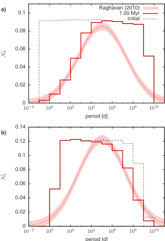
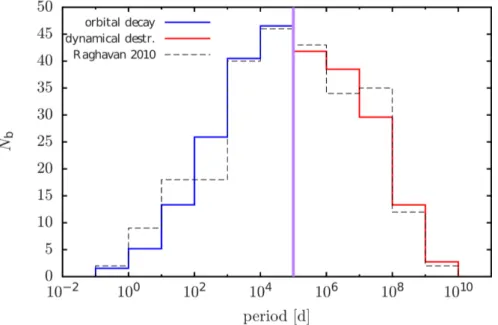
Zunächst wurde die Entwicklung von Doppelsternen in “Orion Nebula Cluster”-artigen (ONC- artigen) Sternhaufen untersucht. Es konnte gezeigt werden, dass die Entwicklung der normalisierten Anzahl an Doppelsternen unabhängig von der initialen Doppelsternrate ist. Dies ermöglicht es, die Entwicklung der Doppelsternpopulationen in ONC-artigen Haufen vorherzusagen, ohne das weitere numerische Rechnungen erforderlich sind. Zusätzlich wurde gezeigt, dass die dynamischen Inter- aktionen vorrangig Doppelsternsysteme massearmer Sterne zerstören, was in Übereinstimmung mit Beobachtungen im ONC zu einer erhöhten Doppelsternrate für massive Sterne führt. Eine Kombina- tion der dynamischen Entwicklung mit dem gas-induzierten Schrumpfen der Orbits von in Gas einge- betteten Doppelsternen wandelt eine logarithmisch gleichverteilte Verteilung der Umlaufzeiten, wie sie in jungen Sternhaufen beobachtet wird, zu einer logarithmisch normalen Umlaufzeitenverteilung um, wie sie in der Feld Population beobachtet wird.

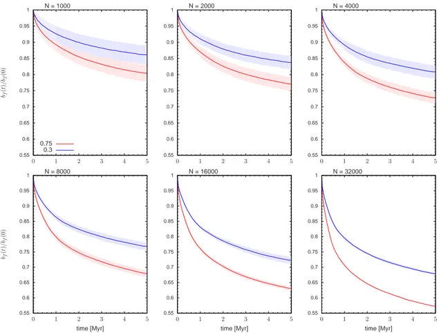
Anschließend wurden die Rechnungen für Sternhaufen mit beliebigen Dichten verallgemeinert, in- dem Simulationen von Sternhaufen mit bis zu achtfach höheren Dichten als im ONC durchgeführt wurden. Es konnte nachgewiesen werden, dass auch in diesen Sternhaufen die Entwicklung der nor- malisierten Anzahl an Doppelsternen unabhängig von der initialen Doppelsternrate ist und das, wie zu erwarten, in Sternhaufen mit höherer Dichte mehr Doppelsterne zerstört werden. Dieser Effekt nimmt jedoch für Sternhaufen mit Dichten von mehr als ≈ 3 × 10

pc

ab. Dies bedeutet, dass es eine Grenze gibt, ab der das Erhöhen der Dichte in den Sternhaufen zu keiner signifikanten Zunahme der Anzahl an zerstörten Doppelsternen führt.

Schließlich wurde untersucht, wie sich Doppelsternpopulationen in Sternhaufen entwickeln, die ihr überschüssiges Gas ausgeworfen haben und in Folge dessen schnell an stellarer Dichte einbüßen. Es wurde gezeigt, dass mit abnehmender Sternentstehungsrate eines Sternhaufens weniger weite Doppel- sterne zerstört und mehr sehr weite gebildet werden. Der Vergleich der Entwicklung der simulierten Sternhaufen und der beobachteten “leacky cluster sequence” legt nahe, dass Sternhaufen mit einer Doppelsternpopulation und einer Sternentstehungsrate von 30% den beobachteten “leaky clusters”

sehr gut entsprechen.

Abstract

Observations of the binary populations in young, sparse clusters have shown, that almost all stars are part of a binary system at the end of the star formation process. By contrast, the binary frequency of field stars only ∼ 50%. Most stars, and therefore most binaries, are formed in dense star clusters.

This rises the question if the natal environments lead to the observed reduction of the binary frequency.

In this thesis this question is addressed using numerical Nbody simulations of binary populations in different star cluster environments.

First the evolution of binaries in ONC-like star clusters has been investigated. It was found that there the evolution of the normalised number of binaries is independent from the initial binary fre- quency. This allows to predict the evolution of binary populations in ONC-like clusters without the need of further numerical simulations. In addition it was found, that dynamical interactions prefer- entially destroy low-mass binaries resulting in a higher binary frequency for high-mass stars in the simulated clusters, in accordance with observation in the ONC. The combination of dynamical evolu- tion with gas-induced orbital decay of embedded binaries is capable to reshape a log-uniform period distribution, as observed in young star clusters, to a log-normal period distribution as observed in the field today.

The modelling has been generalised to clusters with arbitrary densities. Performing simulations for clusters with up to eight times higher densities than before with two different initial binary frequencies, it was shown that the evolution of the normalised number of binaries remains independent of the initial binary frequency. The higher the density in a cluster the more binaries are destroyed as to be expected. However, this effect levels out for clusters with central densities exceeding ≈ 3 × 10

pc

. This means that there is a limit beyond which increasing the binary frequency in the clusters does not lead to significantly more binaries being destroyed.

Finally it was investigated how the binary population evolves in star clusters that have undergone

instantaneous gas expulsion with a resultant fast decrease in stellar density. It was found that the lower

the star formation efficiency of a cluster and therefore the faster the decrease in stellar density, the

less binaries are destroyed during the evolution while at the same time the more very wide binaries

are formed. Comparison of the evolution of the simulated clusters and the observed leaky cluster

sequence shows that clusters including a binary population and a ε = 0.3 match the observations of

leaky-star clusters remarkably well.

Contents

1 Introduction 1

1.1 Star clusters . . . . 3

1.2 Evolution of star clusters . . . . 10

1.3 Binaries . . . . 16

1.4 Gas expulsion . . . . 20

2 Numerical Simulations 27 2.1 Integration . . . . 27

2.2 Individual time steps . . . . 30

2.3 Neigbour treatment . . . . 32

2.4 KS-regularization . . . . 34

2.5 Hardware acceleration . . . . 37

3 Binary populations in ONC-like star clusters 41 3.1 Introduction . . . . 41

3.2 The influence of the cluster dynamics on the binary population . . . . 41

3.3 Orbital decay . . . . 53

3.4 Combination and comparison with observations . . . . 56

3.5 Summary . . . . 61

4 Density-dependence of binary dynamcis 63 4.1 Introduction . . . . 63

4.2 Setup . . . . 63

4.3 Evolution of the binary population in dense star clusters . . . . 64

4.4 Evolution of the period distribution at different densities . . . . 70

4.5 Dependence on the primary mass . . . . 74

4.6 Evolution of the eccentricity and mass-ratio distribution . . . . 77

4.7 Comparison with the observations . . . . 78

4.8 Summary . . . . 82

5 Binary populations in supervirial clusters 83 5.1 Introduction . . . . 83

5.2 General evolution of star clusters after gas expulsion . . . . 85

5.3 Simulation setup . . . . 87

5.6 Summary . . . 112

6 Discussion 115

7 Summary and Conclusions 117

Bibliography 121

A Density-dependence of binary dynamics 129

B Supervirial Cluster Evolution 131

1 Introduction

The most important observations to have shaped our current picture of the binary field population were performed in the early 1990’s. Duquennoy & Mayor (1991) found that the binary frequency of G-type stars in the solar neighbourhood is about 61% and the period distribution follows a log-normal distribution

f (log P ) = C exp

( −(log P − log P )

2σ

)

, (1.1)

over the period range ∼ 10

− 10

d, where P is the period in days (log P = 4.8 ≡ 172yr, σ

= 2 . 3) and C a normalisation constant. A year later, Fischer & Marcy (1992) analysed the binary properties of M-dwarfs in the separation range 0.04 − 10

AU corresponding to periods in the range

∼ 10

− 10

yr and found that the period distribution of M-dwarfs in the solar neighbourhood is also log-normally distributed with a peak between 9yr and 270yr, which is nearly identical to the findings for G-dwarfs. Although the observed binary frequency of M-dwarfs at about 33% is lower than that of G-dwarfs, the properties of the G and M-dwarf binary populations seem very similar. Observations of Raghavan et al. (2010) confirmed this picture. They determined the binary properties of nearby (d < 25pc) solar-type stars ( ∼ F6 − K3) and found that the fraction of binary stars is 58% with a log-normal period distribution (log P = 5.03 and σ

= 2.28).

10⁻¹ 10¹ 10³ 10⁵ 10⁷ 10⁹

frequency

period [days]

Raghavan (2011) Kroupa (1995)

log-uniform

Figure 1.1: Schematic picture of possible initial period distributions. The thick grey curve displays

the log-normal fit to the data of Raghavan et al. (2010), the thick dashed line the Kroupa (1995a),

and the solid line a log-uniform period distribution, which is observed for many young star-forming

regions (see text for references).

With an average age of a few Gyrs, the field population constitutes a dynamically evolved state.

Therefore, dynamical processes have most likely changed the binary properties since the formation of these stars, and the current properties probably differ significantly from the primordial state. To understand the binary formation process, it is insufficient to know the properties of the (old) field population: those of the primordial binary population of to be known.

Connelley et al. (2008) determined the binary properties of the very young populations in Taurus, Ophiuchus, and Orion star-forming regions (excluding the much denser Orion Nebula Cluster). They found that their observed period distribution can be fitted by a log-uniform distribution, which differs significantly from the log-normal distribution in the field (see also Kraus & Hillenbrand (2007)). In these sparse young star-forming regions, it is improbable that dynamical evolution has altered the period distributions in the short period since the stars were formed (see e.g. Kroupa & Bouvier, 2003).

Hence, we can assume that their properties in general match the initial conditions.

In denser regions, indications of an originally log-uniform distribution have also been found. For example, the HST observations by Reipurth et al. (2007) of binaries in the Orion Nebula Cluster (ONC) demonstrate that the semi-major axis distribution deviates from the log-normal distribution and is closer to a log-uniform distribution. Hence, it seems that older binary populations have a log-normal period distribution, while the primordial distribution is likely to be log-uniform.

After the binaries have been processed in the star clusters that have to be released into the field to form the binary population that is observed there today. The most likely process to unbind most binaries is the expansion of the star clusters after they have lost their remnant gas (e.g. Tutukov, 1978;

Hills, 1980; Lada et al., 1984; Baumgardt & Kroupa, 2007) which is also thought to be responsible for the observed leaky cluster sequence for massive clusters (Pfalzner, 2009; Pfalzner & Kaczmarek, in preparation).

From the theoretical side, the binary frequency is the most well-studied binary property (e.g.

Kroupa & Burkert, 2001; Kroupa & Bouvier, 2003; Kroupa et al., 2001; Pfalzner & Olczak, 2007).

It also seems that the evolution of the binary frequency in the ONC depends on the initial binary fre- quency, whereas the evolution of the binary population does not (Kaczmarek et al., 2011). However, the binary population is not only described by the binary frequency but also by the period, mass-ratio, and eccentricity distribution.

Starting with the work of Heggie (1975), it has been realised that binaries can be dynamically dis- rupted by three- and four-body interactions. Wide binaries are generally more affected by dynamical destruction than close ones. The existence of binaries wider than 10

AU in the field is still difficult to explain in models of their origin (Parker et al., 2009).

Performing N-body simulations, Kroupa (1995a,b) showed that to reproduce the observed log-

normal distribution of the field, the initial number of wide binaries has to be significantly higher than

observed, if all binaries are subject to dynamical evolution in a star cluster. This rising distribution was

obtained by inverse dynamical population synthesis, i.e. inverting the effects of dynamical destruction

on the period distribution (see dashed line in Fig. 1.1).

1.1 Star clusters 3

(a) M22 (b) Pleiades

Figure 1.2: a) Image of the M22 globular cluster taken with the Hubble Space Telescope (Copyright:

NASA). b) Image of the Pleiades cluster. Copyright Robert Gendler.

The scope of this thesis is to investigate how binary populations evolve in star cluster models that are motivated by observations of star clusters. In Chap. 3 the evolution of binaries in ONC-like clusters will be studied which will be generalised to cluster of arbitrary densities in Chap. 4. Finally, the evolution of binaries in star clusters after instantaneous gas expulsion will be investigated in Chap. 5 as this ends the evolution of each star cluster.

1.1 Star clusters

1.1.1 Classification

In general, the term “star cluster” denotes a group of several, interrelated stars. Obviously, this definition is very vague and comprises a wide variety of stellar groupings. For this reason, star clusters are usually divided into different groups concerning their shape, mass, age, stellar content and so on.

In this section the definitions concerning gas free clusters will be introduced while embedded star clusters will explicitly be excluded, as they will be treated in Sec. 1.4.

Historically, two different types of star clusters can be distinguished based on their masses, shapes and ages - globular and open (sometimes also-called galactic) clusters. Globular clusters like M22 (see Fig. 1.2a) are very old structures which have their perfect spherical shapes and their small sizes ( ≈ 0 . 1 pc). They usually consist of several 10

− 10

stars and have masses up to 10

M

. In our galaxy ≈ 150 globular clusters are known which can mostly be found in the galactic halo (e.g.

Djorgovski & Meylan, 1993). In contrast to that open clusters like the Pleiades (Fig. 1.2b) are much younger ( < 0 . 3 Gyr) and often show serious deviations from the spherical shape that is observed for globular star clusters. Open clusters are in general much larger than globular clusters (≤ 10 pc) and contain significantly less stars (up to a few thousand). In our galaxy about 1000 open clusters are known today (Dias et al., 2002).

However, the detection of unbound young stellar groupings that do not survive as long as it is

observed for open or globular clusters required to introduce the so-called “stellar associations”. Stellar associations are groups of stars that are only loosely bound or even in the process of being completely dissolved in the near future. Based on the total mass of the association and the type of stars that can be found inside the associations a further distinction is applied for this systems.

T associations are the least massive associations and consist only of low-mass stars that have not reached the main-sequence yet and are still surrounded by their accretion disks. Since stars in this evolutionary phase have first been found in the Taurus-Auriga star forming region (Strom et al., 1975), which is a prototype for a T association, such stars are called T-Tauri stars.

The second more massive type of associations are the so-called R associations which due to their young ages also consist of pre-main sequence stars only. However, as R associations also include intermediate mass stars, they do not only consist of T-Tauri stars but also include Herbig-Ae/Be stars (Herbig, 1960) which are the more massive counterparts of the T-Tauri stars and which produce so-called reflection nebulae by illuminating gas in their surroundings. A typical example for a R association is Mon R2 (Herbst & Racine, 1976).

The last and at the same time most massive type of stellar association are the so-called OB- associations. In contrast to the T- and R-associations these do not exclusively consist of pre-main sequence stars, but also of stars that already settled on the main-sequence, meaning that these stellar groupings are older than the previous two types. Additionally OB-associations contain very massive O and B stars in significant number, which lead to the name of this association type. The nearest OB- association from the sun is the Scorpius-Centaurus Association (Sco-OB2) which includes several thousand stars with masses up to 20 M

(Preibisch et al., 2002).

As can be seen, stellar groupings can be categorised in different ways. However, an objective measure to decide if a stellar grouping is a cluster or an association is still missing. Only recently, Gieles & Portegies Zwart (2011) proposed to use the ratio of age of a stellar grouping and its crossing time Π = age/ t

(see Sec. 1.2.1 for a definition of the crossing time of a stellar grouping) for this purpose. Following their suggestion all stellar groupings with Π < 1 should be designated as stellar association while groupings with Π > 1 should be regarded as star clusters. However, these definition is only based on empirical findings that cannot be substantiated with any physical considerations.

An alternative classification scheme was proposed by Pfalzner (2009), who found that, at least mas- sive clusters with more than 1000 M

, can be divide into two distinct “cluster sequences”, depending on their location in the density radius plot shown in Fig. 1.3. Stellar groupings in the first cluster sequence are called “starburst clusters” and begin their evolution as very small (≈ 0.1 pc), massive ( ≈ 20000 M

) systems that slowly diffuse with time so that after ≈ 20 Myr their sizes have grown to about 1 pc while their total masses remain almost the same. Examples for starburst clusters are the young Arches and Quintuplet clusters, which both are in near vicinity to the galactic centre. How- ever, also the much older χ-Perseus cluster, which is usually categorised as OB-association, has to be designated as being an (old) starburst cluster if the definition by (Pfalzner, 2009) is adopted.

The stellar groupings in the second sequence are called “leaky clusters” and begin their evolution

1.1 Star clusters 5

(a)

Figure 1.3: Observed cluster density as function of the cluster radius for clusters more massive than 10

M

. Taken from Pfalzner (2009).

with the same masses as the starburst clusters but much larger sizes of about 2 pc. During the next 20 Myr the leaky clusters expand to sizes of about 13 pc but at the same time loose a significant fraction of their masses. Examples for leaky star clusters are Cygnus OB2 and Scorpius OB2, which are usually designated as being OB associations.

The evolution of leaky star cluster and the evolution of a primordial binary population inside these clusters will be investigated in Chap. 5. Therefore, the naming convention proposed by Pfalzner (2009) will be applied throughout this thesis.

1.1.2 Models

The most fundamental way to characterise star clusters is to give the complete 6N-dimensional phase- space vector of the cluster consisting of the position and velocity vectors of all stars in the cluster.

However, as star clusters consist of up to several ten-thousand stars this is impracticable when com- paring both observations and simulations of star clusters because of the high number of parameters involved and the dramatic changes of the phase-space vector on short-timescales. Therefore it is convenient to define equilibrium models that describe the clusters with a significantly reduced set of parameters.

In this section of the thesis the most important models of star clusters that are used in theoretical

and observational studies of star clusters will be introduced.

10⁻⁵ 10⁻⁴ 10⁻³ 10⁻² 10⁻¹ 10⁰

10⁻¹ 10⁰ 10¹

ρ/ρmax

r[pc] b= 1pc

r⁻⁵

Figure 1.4: Stellar density distribution resulting from a Plummer model cluster with scale-length b = 1 pc (solid line).

Plummer model

One of the most often used star cluster models is the so-called Plummer-model whose potential is given by

Φ = − GM

√ r

+ b

(1.2)

with the Plummer scale length b and total mass M. The density distribution resulting from this potential is

ρ ( r ) = 3M 4πb

1 + r

b

. (1.3)

From this it can easily be seen, that the Plummer model extends without any borders which of course is not physical.

Originally Plummer (1911) used this potential to fit the observed density profiles of globular clus- ters. Today, the Plummer model is often used for simulations of star clusters in general - regardless if the clusters under consideration are several Gyr old or much younger (e.g. Aarseth et al., 1974;

Kroupa, 1995a; Goodwin & Bastian, 2006; Parker et al., 2009; Allison et al., 2009; Kouwenhoven et al., 2010, and many more). The reason the Plummer model is used that often to set up star clusters in simulations is that, in comparison to other star cluster models (see below), the Plummer model can be described by a set of analytic equations which allows to set up the clusters very easily (Aarseth et al., 1974).

Fig. 1.4 shows the density distribution (Eq. 1.3) of a Plummer model cluster with scale length

b = 1 pc. As can be seen the Plummer model is characterised by a central core, within which the

density is constant. Outside the core, the density of the Plummer density profile starts to decline and

for radii > b the density drops of as r

.

1.1 Star clusters 7

10⁻¹ 10⁰ 10¹ 10² 10³ 10⁴ 10⁵

10⁻¹ 10⁰ 10¹

ρ

r[pc]

Figure 1.5: Stellar density distribution of the singular isothermal sphere.

The isothermal sphere

The present standard picture of star formation states, that stars form out of self-gravitating molecular clouds (Larson, 2003), which can be approximated as being isothermal spheres. As also the star clusters form out of this molecular clouds, it seems reasonable to assume that also star clusters can be approximated as being isothermal spheres.

The gravitational potential of the so-called singular isothermal sphere (singular due to the singu- larity at the cluster centre) is given by

Φ ( r ) = 2 σ

ln ( r ) + const . (1.4)

where σ = p

k

T / m is the velocity dispersion inside the cluster. Applying Poisson’s equation yields the stellar density distribution

ρ ( r ) = σ

2πGr

. (1.5)

The mass of the cluster inside a given radius r is given by M ( r ) = 2σ

r

G . (1.6)

The velocities of the stars in the isothermal spheres are given by the Maxwellian velocity distribution dn ∝ exp

− | v |

2σ

d

v (1.7)

independently of the position in the sphere.

Fig. 1.5 shows the stellar density distribution of an isothermal sphere. In contrast to the Plummer

model, which exhibits a central core, within which the density is constant, the isothermal sphere has a

Figure 1.6: Projected density profiles for the King models (from King, 1967). The curves show the logarithm of the projected density (normalised to the central value) for selected values of the concentration parameter c (marked along the curves). For each case an arrow provides the location of the relevant truncation radius r

.

central cusp, within which the density remains raising in contrast to a core where the density becomes constant (see Sec. 1.1.2). As a result, the density in the central parts of an isothermal sphere are very high leading to many stellar interactions.

The isothermal sphere has so far not often been used in investigations of the dynamics of star clusters. One of the reasons for this is that the singular isothermal sphere due to its central singularity features very high densities in its centre, which can lead to numerical problems if such a cluster is simulated. Another reason isothermal spheres in simulations are not used in general for simulations is that strictly speaking, isothermal spheres do not have any boundaries regarding the size and mass.

However, observed star clusters obviously are finite objects. As a result, even if a cluster is set up as isothermal sphere in virial equilibrium, the cluster will expand making it a not a good candidate if the evolution of clusters in equilibrium shall be investigated.

However, isothermal spheres have also been used successfully in star cluster simulations. For example the cluster model introduced by Olczak et al. (2006) uses a modified version of the isothermal spheres to model the initial state of the Orion Nebula Cluster. This cluster model has been proven to evolve to the same state as is observed in the ONC today (see also Olczak et al., 2008, 2010) and is used in Chap. 3 for investigating the evolution of a primordial binary population in ONC-like clusters.

King models

The isothermal sphere and Plummer model can be used straight-forwardly to set up star clusters in

simulations, because they can be described with simple analytic functions (e.g. Aarseth et al., 1974,

and Sec. 1.1.2 and Sec. 1.1.2). However, strictly speaking, both models are only applicable for clusters

that are either very young (isothermal sphere) or very old (Plummer). A star cluster model that is

1.1 Star clusters 9 applicable to star clusters of any age is the family of King models, which were initially introduced to fit the density profiles of globular clusters (King, 1962), but can also be used for much younger cluster like the ONC (Hillenbrand & Hartmann, 1998).

Theoretically, the King models can be derived by limiting the distribution function of the isothermal sphere by setting it to zero outside the desired tidal radius of the cluster, which sets the size of the cluster (see Binney & Tremaine, 2008, for a complete introduction into King models). Integrating this distribution function over the complete velocity space yields the density as a function of the cluster potential of the King model clusters which is given by

ρ

( Ψ ( r )) = ρ

"

e

erf

p Ψ ( r ) σ

!

−

r 4Ψ ( r ) π σ

1 + 2Ψ ( r ) 3σ

#

, (1.8)

where Ψ ( r ) is the relative potential of the cluster, σ a parameter that should not be mistaken for the velocity dispersion of the cluster and erf the Error function. As can be seen In comparison with the corresponding density distributions of the Plummer and isothermal sphere model, the density distri- bution of King model cluster is much more complicated and to setup a star cluster in the simulations one has to numerically integrate the Poisson equation for Ψ (for more details see Binney & Tremaine, 2008).

Basically, the King models can be parametrised by the ratio of W

= Ψ(0)/σ or their concentration

c = log

( r

/ r

), (1.9)

where r

is the tidal radius of the cluster, beyond which the cluster ends and

r

= s

9σ

4πGρ

(1.10) is the King radius of the cluster, which gives the size of the core of the model. The concentration therefore gives the ratios of the cluster core size to its initial size where higher values of c denote more concentrated clusters. In the limit W

→ ∞, c → ∞ the King models go over to the isothermal spheres, while for lower values of W

and c, the resulting clusters become less extreme. For example, the ONC can be fitted by a King model cluster with W

= 9 (c ≈ 2 . 1) while the Plummer model can be approximated by a King model with W

= 4 (c ≈ 0 . 8). Fig. 1.6 shows a series of King models with concentration factors in the range from 0.5 − 2.5. As can be seen the size of the core with respect to the size of the complete cluster decreases the larger c becomes.

In contrast to the Plummer and isothermal model, where the velocity dispersion is constant thought

the cluster, the velocity dispersion in King model clusters is a function of the distance to the cluster

centre. The larger the distance to the cluster centre is, the lower is the velocity dispersion.

1.2 Evolution of star clusters

Although on first sight star clusters appear to be rather static objects, they undergo serious evolution during their lifetimes. In the following section some important processes acting in and on star cluster will be summarised.

1.2.1 Two-body relaxation

The simplest way to treat self-gravitating stellar systems like star clusters is to assume, that they are

“collisonless systems” in which the trajectories of the stars are dictated by the smoothed out potential of the complete system. While this approximation can safely be applied for galaxies (N ≈ 10

1, t

= 100Myr , t

≈ 4 × 10

Myr, age ≈ 10Gyr), it fails to explain the evolution of star clusters as there the gravitational interactions between the stars with their neighbours becomes important. The reason for this is that due to this stellar encounters the trajectories of the stellar members are deflected from the path they would have if no encounters would have taken place, although this changes are mostly very small (the effect of strong encounters will be discussed in Sec. 1.2.5).

However, during their lifetime the stars in a cluster will undergo many of such weak encounters which means that after some time all stars in the cluster will have left their initial trajectories and follow paths that are specified by their neighbours instead of the gross cluster potential. The time- scale after which this happens can be calculated by determining the number of times a star has to cross the star cluster so that the many small interactions have changed the velocity of the star by an amount comparable to its initial velocity (e.g. Binney & Tremaine, 2008). This time is called relaxation time of the cluster and can be approximated by

t

' 0 . 1N

ln N t

, (1.11)

where N is the number of particles in the systems and t

= R / v is the crossing time of the system (R is the diameter of the system and v the mean velocity of the stars). The crossing time gives the average time a star in the cluster needs to cross the complete cluster and is the shortest time, within which significant dynamical changes in the clusters, like changes of the cluster shape, can occur. Instead of calculating this relaxation time, often the half-mass relaxation time (e.g. Binney & Tremaine, 2008) is given because it can be constrained easier by observation than the regular relaxation time. It is calculated by

t

= 0 . 78Gyr ln( λ N )

1M

m

M 10

M

r

1pc

(1.12) where ln ( λ N ) is the so-called Coulomb logarithm, m the mean stellar mass in the cluster, M the total mass and r

the half-mass radius. The Coulomb logarithm is often found in formulae for scatter- ing rates from 1 / r potentials, such as the gravitational potential of a point mass or the electrostatic potential of a point charge.

Two-body relaxation is of major importance for the evolution of stellar systems with ages that

1.2 Evolution of star clusters 11 exceed the relaxation time of the system. Therefore two-body relaxation had a significant influence on old globular clusters (N ≈ 10

, t

= 0 . 5Myr , t

= 0 . 5Gyr, age ≈ 10Gyr, based on values from Harris (1996)), and old open clusters (N ≈ 10

, t

= 1Myr , t

= 15Myr, age ≈ 0 . 3Gyr, based on values from Piskunov et al. (2007)), while it has not been of great importance for much younger cluster like the Orion Nebula Cluster (N = 4000, t

= 0 . 3Myr , t

= 15Myr, age ≈ 1Myr, based on values from Hillenbrand & Hartmann (1998)). However, this does not mean that stellar encounters are of no importance in these clusters. As will be shown later, strong encounters can remove stars from star clusters (Sec. 1.2.5), alter the properties of stellar disks in star clusters (Pfalzner et al., 2006;

Olczak et al., 2006, 2010; Steinhausen et al., 2012) and alter binary system, which is investigated in this thesis.

1.2.2 Thermodynamics of self-gravitating systems and Core collapse

In analogy to ideal gases, the temperature of a given stellar system can be defined by the relation 1

2 m v ¯

= 3

2 k

T , (1.13)

where m is the stellar mass, ¯ v the mean velocity of the stars and k

is Boltzmann’s constant. In general the mean velocity in a stellar cluster depends on the location of the star in the stellar cluster, therefore also the temperature in general depends on the position (the isothermal sphere displays an exception).

The mass-weighted mean temperature is ¯ T = ^R d

xρ ( x ) T / ^R d

xρ ( x ) , where ρ ( x ) is the density, and the total kinetic energy of a system of N identical stars is therefore

K = 3

2 Nk

T ¯ (1.14)

In a stationary system the virial theorem then states that the total energy of the system is E = − K, so E = − 3

2 Nk

T ¯ . (1.15)

Therefore the heat capacity of an self-gravitating stellar system is C = dE

d ¯ T = − 3

2 Nk

, (1.16)

which is negative. This means that the system increases in temperature if it looses energy.

This causes self-gravitating stellar systems to collapse into singularities if they are in contact with heat baths which have a lower temperature than the self-gravitating system because energy is flowing from the hotter system into the cooler heat bath. On contrary self-gravitating stellar systems will expand if they are in contact with heat baths that have a higher temperature.

It turns out that star clusters usually also show this behaviour which leads to a phenomenon called

core collapse. The mean stellar velocity in star clusters (the isothermal sphere again marks an excep-

tion) usually depends on the position within the cluster with the stars in the cluster core having higher speeds than in the outer cluster parts. This means that the temperature in the cluster core is higher than in the cluster outskirts. Therefore energy will flow from the cluster core to the outer cluster parts in the form of ejected stars. As this energy flow increases the temperature within the cluster core due to the negative heat capacity, it decreases in size to return to virial equilibrium. Because the temper- ature gradient of the core and the outer cluster parts steepens due to this process, it accelerates itself potentially leading to the formation of a singularity at the cluster centre.

Early simulations of the evolution of globular clusters using the Fokker-Planck or fluid approxi- mations did not include any processes to stop core collapse (e.g. Hénon, 1961; Sabbi et al., 2011, translation) so that they all led to the formation of a singularity after about 16 initial half-mass re- laxation times (Eq. 1.12). However, this time should only be taken as a crude estimate of the “core- collapse” time, as it heavily depends on the cluster density profile and mass function, that is used for the computations.

In more realistic computations core collapse does not proceed to this extreme state. To halt core collapse, an energy source is needed that pumps energy into the core. Due to the negative heat capacity of self-gravitating system, the temperature of the core decreases so that the temperature gradient between the cluster core and the outer cluster parts diminishes. If both temperatures become the same, the heat flow vanishes and the core collapse has stopped.

A natural energy source, that could halt the core collapse in star clusters are binary stars. Their interactions with other core members have been already recognised by Hénon (1961) as possible process to stop core collapse, however it took almost 20 years until Sugimoto & Bettwieser (1983) were able to consistently include their influence on the evolution of star clusters into the computations.

1.2.3 Influence of the galactic potential

The stellar cluster models described in Sec. 1.1.2 are often assumed to be isolated to simplify the calculations. In reality however, star clusters are embedded in their parent galaxies. Therefore stars do not only feel the gravitational potential resulting from the other stars in the cluster, but also the potential of the overall galaxy, which has important implications for the structure of star clusters.

To derive the radius beyond which a star will no longer be bound to its star cluster but to the hosting galaxy it is convenient to change to a coordinate system that rotates with an angular velocity Ω so that the galaxy and the cluster are standing still. In this coordinate system, the usual total energy is not conserved but the Jacobi integral

E

= 1

2 mv

+ Φ ( x ) − 1

2 m | Ω × x |

= 1

2 mv

+ Φ

( x ), (1.17)

with Ω = [ 0 , 0 , Ω ] and the term −

m | Ω × x |

being something like the “potential energy” giving rise

to the centrifugal forces present in the rotating coordinate system.

1.2 Evolution of star clusters 13 Next one has to determine the saddle point of Φ

that lies between the cluster and the galaxy. This means that at ( x

− r

, 0 , 0 ) the potential has to fullfill the following condition

∂ Φ

∂ x

x=x−r_J

= 0 (1.18)

The effective potential generated by the cluster and the galaxy separated by a distance d can be written as

Φ

( x ) = − G

m

| x − x

| + m

| x − x

| + 1 2

m

+ m

d

|e

× x|

(1.19) Combining Eq. 1.18 and Eq. 1.19 then gives

0 = 1 G

∂ Φ

∂ x

x_cl−r_j

= m

( d − r

)

− m

r

− m

+ m

d

d

1 + m

/ m

− r

(1.20)

In the current context m

so that r

d and it is possible to expand ( D − r

)

in powers of r

/ D:

0 = m

d

1 + 2r

D + ...

− m

r

− m

d

+ m

+ m

d

r

(1.21)

So to the first order in ( r

/ D ) it follows that r

=

m

m

( 3 + m

/ m

)

d u m

3m

d (1.22)

The here derived radius r

is often called the Jacobi limit or the Jacobi radius. It displays a rather good estimate of the tidal radius r

of an star cluster in it’s host galaxy

1.2.4 Stellar mass loss

At the end of their life most stars loose significant amounts of their mass due to stellar winds or in the extreme case through supernova explosions. Most of this material is likely to escape the cluster as the velocities of the winds (for massive stars they can be up to ≈ 2000km s

) usually exceeds the escape velocity of the cluster (for example v

= q

GM

r

≈ 3km s

for the ONC) which results in a loss of cluster mass without the need of reducing the number of stars in the cluster (disregarding supernovas which do remove stars).

Usually the effect of lowering the stellar mass in the cluster is to widen the stellar orbits of the stars without changing the shape of the orbits because the timescale of the mass loss is much longer than the crossing time of the cluster, so that it can adapt to the new potential adiabatically (see Sec. 1.4).

As long as the cluster is treated to be isolated, it could grow without any boundaries without loosing

any stars (neglecting supernovas or the like). If however, the cluster is placed into the tidal field

of an galaxy, the cluster will loose stars if they pass the tidal or Jacobi radius r

of the cluster (see

Sec. 1.2.3).

1.2.5 Evaporation and ejection

Encounters of stars in a star cluster potentially remove stars from the cluster by two distinct processes.

(i) A single, strong encounter with another star or with a binary can raise the energy of one star by such an amount, that it directly leaves the star cluster. This process is called ejection. (ii) Multiple, weak encounters of a star with many other stars can gradually raise the energy of the star, so that it can leave the star cluster. This process is called evaporation.

To be able to estimate the importance of these two processes, the ejection and evaporation time- scales will be given, which denote the time each process would need to completely dissolve the cluster

t

= − 1

N dN

dt

. (1.23)

The ejection time-scale of an isolated cluster with a Plummer density distribution consisting of single-mass stars only was determined by Hénon (1960) to be

t

≈ 10

ln(λ N ) t

(1.24)

where ln( λ ) is before mentioned Coulomb logarithm and t

is the half-mass relaxation timescale (see Eq. 1.12). Including a mass function in the calculations significantly increases the effectiveness of the ejection process as massive stars tend to eject a high number of lower mass stars. Henon (1969) found that the ejection timescale is reduced by a factor of about 30 when including a mass function in the calculations.

While the ejection timescale can, in principle, be evaluated analytically, the determination of the evaporation timescale requires using numerical calculations. The reason for this is that while for the ejection only a single encounter has to be considered, evaporation emerges from millions of encoun- ters of a star with the other stars in the cluster which, in very small steps, rise the energy of the star so that it possibly can leave the cluster. Using Fokker-Planck calculations Spitzer (1987) determined the evaporation timescale of an isolated single-star cluster to be

t

= 300t

, (1.25)

which is about 30 times shorter than ejection time scale (ln ( λ N ) ≈ 10 for typical clusters). However,

the timescale given in Eq. 1.24 and Eq. 1.25 should be treated with caution because the calculations

used to acquire them did not include all physics present in star clusters, which might have an effect

on these. For example by including the effect by an external tidal field on the cluster both timescales

can be reduced by a factor of ten (Spitzer, 1987).

1.2 Evolution of star clusters 15 1.2.6 Energy equipartition and mass segregation

All processes that have been discussed so far in this chapter can work in clusters, that consist only of single stars. However, not all stars have the same mass, but show a wide range of masses from the Hydrogen-burning limit (0 . 08M

) to the theoretically accepted maximum stellar mass of 150M

up to which stars are stable. However, stars with even higher masses have been detected recently (Crowther et al., 2010).

By allowing the stars in a cluster to have different masses, the kinetic energy of a star will not only depend on the position of the star, but also on its mass. Encounters will therefore tend to establish energy equipartition between the lighter stars and the more massive ones. However, energy equipar- tition in self-gravitating systems does not work exactly the same way as in ideal gases, where only the kinetic energy has to be considered. To enlighten this, consider a self-gravitating system with potential Φ ( x ) consisting of two populations of stars with masses m

and m

and m

>> m

. The mean energy per star in both population is then given by h E i

= m

1/2v

+ Φ(x)

i

where hi

denotes the average over the complete population i and v is the average velocity of the stars. Encounters do not lead to h E i

→ h E i

on throughout the cluster but only locally. This means that if the energy of the heavier stars is higher than the energy of the less massive stars at a given location x (so they have higher kinetic energies), then they will transfer part of their energy with the lower mass stars.

However, by loosing orbital energy the heavier stars will sink deeper into the potential Φ(x) so that they have to speed up to keep their new energy after the energy transfer conserved. That means that due to energy equipartition, the kinetic energy of massive stars increases in contrast to what would be assumed at first glance.

Energy equipartition therefore leads to the massive stars being more centrally concentrated than the lower mass stars in the cluster. This state is often called “mass segregation” and is observed in many star clusters (Hillenbrand & Hartmann, 1998; de Grijs et al., 2002; Gouliermis et al., 2004). Since also very young cluster like the ONC show evidence for mass segregation the question arises, if star clusters are born in a mass segregated state or if the energy equipartition is responsible.

Performing Nbody simulations of star clusters in virial equilibrium Bonnell & Davies (1998) could show that the degree of mass segregation, that is observed in the ONC today can only be explained if the cluster was already initially mass segregated. In contrast to that Allison et al. (2009) found, that no initial mass segregation is needed to explain the mass segregation of the ONC, if the cluster was initially in a clumpy, subvirial state. Olczak et al. (2011) could even generalize this by dropping the need for a clump structure of the clusters.

Because energy equipartition causes an inward motion of massive stars, it can significantly speed

up the core collapse. While in the single-mass case, core collapse occurred after about 16t

(see

Eq. 1.12, it can appear after 2 − 4t

if a proper mass function is used in the simulations.

1.3 Binaries

Binary stars are pairs of stars, that are energetically bound, meaning that their internal or binding energy is smaller than zero:

E

= 1

2 m

v

+ m

v

− Gm

m

| r

|

= 1

2 µ r ˙

− Gm

m

|r

| < 0, (1.26)

where m

, m

are the masses of the stars, v

, v

are the velocities in their centre of mass rest frame and r

the separation vector between the two stars. The orbits of the two stars follow Kepler ellipses with the eccentricty

e = s

1 + 2

L

E

G

( m

+ m

)

, (1.27)

where L = r

× p

= r

× µ r ˙

is the angular momentum vector of the orbit. For binaries the eccentricity is always < 1. The semi-major axis of the orbit is given by

a = L

GM ( 1 − e

) (1.28)

With this the periastron distance r

(minimum separation between the two stars) and the apoastron distance r

(maximum separation) are given by

r

= a ( 1 − e ), (1.29)

r

= a (1 + e ). (1.30)

Currently several binary formation scenarios are discussed by the community which can be divided into three groups: i) scenarios based on the fragmentation of collapsing cores, ii) fragmentation inside a protostellar disk and iii) dynamical formation. The first two scenarios are obviously linked to the star formation process itself and binaries formed by either of these scenarios can therefore be safely be regarded as being primordial. However, also dynamically formed binaries can be regarded as being primordial as long as they are formed during as long the star formation proceeds in the cluster.

The first formation scenario for binaries occurs very early in the star formation process, when

subclumps inside molecular clouds begin to collapse (which are then called collapsing cores), because

the local gaseous pressure support is not able to balance out the force of gravity which occurs if

the subclumps have masses exceeding the local Jeans mass. The first core fragmentation scenario

has been investigated by Hoyle (1953), who assumed that during the collapse of the cores, further

fragmentation of the core occurs, as long as the gas remains optically thin and is able to efficiently

cool. The reason for this is that the Jeans mass decreases with increasing density and increases with

temperature.

1.3 Binaries 17 More recent core fragmentation scenarios have found that collapsing, bound gas clumps will frag- ment depending on product of the ratio of the thermal to gravitational energy α = 5c

R / GM and the ratio of rotational to gravitational energy β = Ω

R

/ 3GM, where c

is the sound speed, R the core radius, M the core mass and Ω the orbital frequency of the core. Initially it was thought that cores with α β < 0 . 12 will inevitably fragment Inutsuka & Miyama (1992), however it turned out that the cores must additionally obey α < 0.5 to be able to fragment (Tsuribe & Inutsuka, 1999).

Another class of binary formation scenarios relying on the fragmentation of the cores are the so- called turbulent fragmentation scenarios. These scenarios assume that turbulence can lead to overden- sities or filementary structures within the bound cores, that will collapse and form a separate entity inside the core. Recent work by Offner et al. (2009) and Offner et al. (2010) implies, that the turbulent fragmentation is the dominant mode of low-mass binary formation.

The next family of binary formation scenarios is based on the fragmentation of massive protostel- lar/accretion disks. As these form after the core has already collapsed significantly, the disk frag- mentation scenarios take place later in the formation of the stars than the before mentioned core fragmentation scenarios. Disk fragmentation has recently gathered more attention as it is now becom- ing obvious, that the feeding of the disk by the surround envelope of the star (Kratter et al., 2008, 2010) is a efficient way to induce instabilities in the disk and that protostellar disks can be much more massive, that has been thought before (Andrews & Williams, 2007). Both findings significantly improve the efficiency for the formation of binaries in disks, making it more important as it has been expected before.

Disk fragmentation is a promising process to explain close binaries, that are only rarely formed in the core fragmentation scenarios. The reason close binaries can form through disk fragmentation is that the new stars forming in the disks have directly from the beginning relatively small separations to the central star (several 100AU) and can wander inside the disk, as it has already been found for planets (Goldreich & Tremaine, 1979).

The last family of binary formation scenarios is based on the dynamics of stars in their natal en- vironments, namely star clusters (Lada & Lada, 2003). The so-called competitive accretion model (Bate, 2000; Bonnell et al., 2003; Clark & Bonnell, 2004; Bonnell et al., 2008) states that during the formation of a star cluster, many stars form which will accrete from the overall gas present in the cluster. During this period binaries will form by processes already mentioned above (e.g. via core and disk fragmentation mentioned above) or by other processes like the disk-assisted capture Moeckel &

Bally (2007)). An additional way to form binaries also after the star formation has been completed is the formation of binaries during a three-body interaction (Heggie, 1975). To form a binary during such an interaction, the initially positive binding energy of two unbound star, has to be lowered be- low zero. This is accomplished by transferring the superfluous energy to the third star, which will afterwards leave the system with a increased velocity.

As has been shown above, the formation of stars and binaries is associated with dense molecular

clouds and is not accessible by observations because the extinction due to the gas in this regions is

too high. Therefore it is not possible to determine directly by which formation scenarios the binaries actually form. However, what can be done is to observe the binary populations resulting from the star formation process and compare them to the predictions from the theory.

The most important observations to have shaped our current picture of the binary field population were performed in the early 1990’s. Duquennoy & Mayor (1991) found that the binary frequency of G-type stars in the solar neighbourhood is about 61% and the period distribution follows a log-normal distribution

f ( logP ) = C exp

( −( logP − logP )

2σ

)

, (1.31)

over the period range ∼ 10

− 10

d, where P is the period in days (log P = 4 . 8 ≡ 172yr, σ

= 2.3) and C a normalisation constant. A year later, Fischer & Marcy (1992) analysed the binary properties of M-dwarfs in the separation range 0 . 04 − 10

AU corresponding to periods in the range

∼ 10

− 10

yr and found that the period distribution of M-dwarfs in the solar neighbourhood is also log-normally distributed with a peak between 9yr and 270yr, which is nearly identical to the findings for G-dwarfs. Although the observed binary frequency of M-dwarfs at about 33% is lower than that of G-dwarfs, the properties of the G and M-dwarf binary populations seem very similar. Observations of Raghavan et al. (2010) confirmed this picture. They determined the binary properties of nearby (d < 25pc) solar-type stars (∼ F6 − K3) and found that the fraction of binary stars is 58% with a log-normal period distribution (log P = 5 . 03 and σ

= 2 . 28).

While these studies draw a very consistent picture of binaries it is not compatible to observations in star cluster. The most serious differences are that the binary frequency is much higher in (sparse) clus- ters (Leinert et al., 1993; Ghez et al., 1993; Reipurth & Zinnecker, 1993; Kraus & Hillenbrand, 2007) and the period distribution seems to be log-uniform in young clusters (Kouwenhoven et al., 2007;

Kraus & Hillenbrand, 2007; Reipurth et al., 2007; Connelley et al., 2008). In contrast observations of the binary frequencies in dense star clusters like the ONC (Prosser et al., 1994; Petr et al., 1998;

Duchêne, 1999; Simon et al., 1999; Beck et al., 2003; Köhler et al., 2006; Reipurth et al., 2007) have shown, that the binary frequency in these clusters is comparable to the binary frequency in the field.

These findings rise the question why the binary popultions in the star clusters and the field differ. A possible explanation is that the binaries, are influenced by the natal environment. A process naturally acting in star clusters that is capable to change binaries are the before mentioned three-body interac- tions. The general effect of three-body interactions onto a binary can be expressed by the relative energy change of the binary, ∆,

∆ = E

− E

E

, (1.32)

where the primed variables denote the values after the scattering event. If ∆ > 0 the internal energy of the binary has become more negative which means that it is harder bound than before the interaction.

From the conservation of energy it follows that the energy of the third body E

increases during the

interaction, so that its final velocity exceeds its initial velocity, V

> V . The inverse process with

1.3 Binaries 19

Figure 1.7: From Hut & Bahcall (1983). A three-body scattering event. It is a resonant exchange and the sequence of integrations is summarised in the pictogram at the upper left.

∆ < 0 leads to a less tightly bound binary and a slower third body (V

< V ).

One can introduce two types of binaries based on the relation of binding energy and relative kinetic energy (Heggie, 1975; Hills, 1975). Binaries with |ε | > ( m

+ m

) m

V

/( m

+ m

+ m

) are called hard binaries which are hardened by three-body scatterings and binaries | ε | < ( m

+ m

) m

V

/( m

+ m

+ m

) are called soft because of their fragility to such encounters.

Soft binaries become softer in a three-body interaction. Here three different processes can be distinguished. First, in a fly-by the “intruder” gets close to the binary, softens it (∆ < 0) and escapes to infinity again. The second process is called ionisation which happens when the “intruder” causes a relative velocity change large enough, that the binary becomes unbound. The third process is the exchange process (see Fig. 1.7) where the intruder changes place with one of the binary components due to a very close encounter.

The effect of three-body scattering on hard binaries is that the binary gets even harder. Two different regimes for three-body scatterings can be distinguished, one for close interactions r

≤ a (r

is the minimum separation of the third body and the binary, a the semi major axis of the binary) and one for wide interactions where r

>> a.

In the close interaction case the amount of energy exchanged in an interaction is of the order of | ε | .

Also here two different outcomes are possible. First the intruder may get a positive amount of energy of order | ε | which vastly increases the speed of the intruder and hardens the binary considerably. In contrast, if the intruder looses energy in the interactions, it will become bound to the binary and another interaction will take place. Such interactions can occur repeatedly for a long period and lead to rather stable configurations called resonances. In this case exchanges of a binary component and the intruder are common. The probability for an exchange in an equal mass system is 2/3, in an unequal mass system it is by far more probable that the lowest mass component is ejected in this process.

The same processes take place in the wide interaction case, but the amount of exchanged energy is greatly reduced. Also an exchange interaction is not possible in the resonance case which is now not called resonance anymore but “hierarchical”.

However, as three-body and even higher order interactions occur very often in star clusters during their lifetimes, it is not possible to calculate the changes of the binary population in the clusters analytically but numerical simulations have to be performed. Several authors studied the evolution of binary populations in star clusters of different kind (e.g. Aarseth, 1971; Kroupa, 1995a; Kroupa et al., 1999; Kroupa & Burkert, 2001; Kroupa & Bouvier, 2003; Pfalzner & Olczak, 2007; Parker et al., 2009; Kouwenhoven et al., 2010). Numerical investigations of the dynamical evolution of binaries in star clusters started in the 70’s with the development of the first N-body codes (e.g. Aarseth, 1971).

The early works concentrated on the formation of binaries in star clusters with initially pure single stellar systems. Only in recent years simulations have been performed to investigate the evolution of a primordial binary population. For example, Kroupa et al. (1999) simulated the evolution of ONC- like star cluster models where all stars initially were part of a binary system, i.e. a primordial binary frequency of 100%. They showed that the cluster evolution destroys wide binaries quite efficiently leading to a reduction in the initial binary fraction as the cluster evolves.

A different approach to calculate the evolution of star clusters is to use the Fokker-Planck equation, which describes the evolution of the distribution function of a star cluster due to encounters in the cluster. In cases where only single stars are present in the clusters, the diffusion coefficients, which give the mean changes of the distribution function due to encounters, can be acquired quite easily.

However, if also binaries are present in the clusters the cross sections of the different outcomes of three body interactions have to be known which have been determined by several authors by calculating immense numbers of three-body interactions (Hut, 1983b; Hut & Bahcall, 1983; Hut, 1983a, 1993).

This thesis displays a continuation of this studies with the focus on the creation of the field binary population in cluster models being motivated by observed clusters.

1.4 Gas expulsion

The generally accepted view of cluster formation is that star clusters originate from Giant Molecular

clouds (GMCs). With typical masses of 10

− 10

M

and typical diameters of 10 − 100pc GMCs

1.4 Gas expulsion 21 display immense reservoirs for star formation. However, observational evidence exists that only a minor fraction of the total cloud mass is actually converted into stars. One reason for this is that the vast majority of the material in the GMC is supported against gravitational collapse either through turbulence or magnetic fields (Arons & Max, 1975; Blitz, 1993; Myers & Goodman, 1988). Only in the densest parts of the clouds, the so-called dense cores gravity dominates. This means that only a minor fraction of an entire GMC is capable to form stars, so that the overall star formation efficiency (SFE) in a GMC is at most a few percent (Lada & Lada, 2003; Clark & Bonnell, 2004).

However, even within the dense cores the SFE does not reach 100% because the star formation process turns out to be rather ineffective. The radiation and stellar winds of newly formed (proto-) stars heat up the surrounding gas making it more difficult for the gas to collapse into new stars or accrete onto already formed ones. In fact material can even become unbound and leave the cluster if a sufficient amount of energy is pumped into the gas. The energy needed to remove all gas from a cluster is approximately (Adams, 2000)

E = k GM

R ≈ 4 × 10

erg

M 1000M

R 1pc

, (1.33)

with k being a numerical constant of the order one describing the structure of the gas cloud. So to unbind all gas in a typical massive young star cluster (M

= 15000M

, R = 10pc) with an assumed SFE of 30% an energy of more than E ≈ 10

erg has to be inserted into the gas. Stellar winds and the ionizing radiation of young stars are not capable to release enough energy to instantly free all gas from the cluster and therefore turn out not to be the major processes that remove the gas from massive clusters. In contrast, supernova explosions can easily unbind the complete amount of gas from the clusters as their energy input is about 10

erg (Khokhlov et al., 1993). Lower mass clusters, in which no massive star formation takes place and which are therefore void of supernovas, are observed to become gas-free (Palla & Stahler, 2000) at some point. In those clusters the stellar winds and the ionizing radiation of the young stars become more important.

Summarising the formation and early evolution of star clusters is charaterised by an transition from a system consisting mainly of gas and a minor fraction of stars to a system that more or less exclusively consists of stars. During this transition, the potential of the clusters changes significantly possibly accompanied with severe changes of structure of the clusters. To study this in more detail several studies have been performed to determine which fraction of stars stays bound after the gas has been removed from the clusters and how this fraction depends on the gas expulsion process, the star formation efficiency, the cluster density profile and so on.

The most basic description of the gas expulsion process starts from the evolution of the energies of clusters in virial equilibrium before gas loss (Hills, 1980). Before a cluster looses its gas component, the kinetic and potential energy of the cluster are given by T

=

M

v

and W

= GM

/2R

, where M

= M

( 0 ) + M

( 0 ) is the initial total mass of the cluster,

v

= GM

/ 2R

the velocity disper-

sion of the stars and R

the effective radius of the cluster. For equal mass stars, R

would be given by