Time efficient optimization of instance based problems with application to tone onset detection

SFB 823

Time efficient optimization of instance based problems with application to tone onset

detection

Discussion Paper

Claus Weihs

Nr. 85/2016

Time efficient optimization of instance based problems with application to tone onset detection

Nadja Bauer^a,∗, Klaus Friedrichs^a, Claus Weihs^a

aDepartment of Statistics, TU Dortmund University, D-44221 Dortmund, Germany

Abstract

A time efficient optimization technique for instance based problems is proposed, where for each parameter setting the target function has to be evaluated on a large set of problem instances. Computational time is reduced by beginning with a performance estimation based on the evaluation of a representative subset of instances. Subsequently, only promising settings are evaluated on the whole data set.

As application a comprehensive music onset detection algorithm is intro- duced where several numerical and categorical algorithm parameters are opti- mized simultaneously. Here, problem instances are music pieces of a data base.

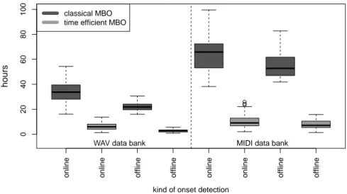
Sequential model based optimization is an appropriate technique to solve this optimization problem. The proposed optimization strategy is compared to the usual model based approach with respect to the goodness measure for tone onset detection. The performance of the proposed method appears to be competitive with the usual one while saving more than 84% of instance evaluation time on average. One other aspect is a comparison of two strategies for handling categorical parameters in Kriging based optimization.

Keywords:

model based optimization, instance optimization, Kriging, onset detection, categorical parameters

1. Introduction

Parameter optimization is an important issue for industrial optimizations as well as for computer based applications. The established industrial optimization approach is based on a design of experiments where the trials are conducted according to a pre-defined plan [1]. The so called plan matrix should satisfy some special statistical criteria (like A- or D-optimality). After evaluation of the plan a relationship between the target variable and the influencing parameters

∗Correspondence to: Department of Statistics, Vogelpothsweg 87, D-44227 Dortmund, TU Dortmund University, Germany. Tel.: +49231 755 7222; Fax: +49231 755 4387.

Email address: bauer@statistik.tu-dortmund.de(Nadja Bauer)

is fitted by a regression model. Usually, a linear model with interactions and quadratic terms is used for this task. The optimal parameter setting is then defined as the point with best model prediction value.

Despite the long success history of the optimization approach mentioned above [2, p. 467] it shows two essential weak points. First, the real experiments are often time and cost consuming. In some cases the real processes can be replaced by a sophisticated computer simulation. However, even one run of such simulation can take several days or months [3]. Hence, it is crucial to avoid trials in not promising areas and conduct them in the neighborhood of the supposed optimum instead. Second, the assumptions of the linear model are often violated so that it does not represent the true complex relationship between the target and the influencing factors. The sequential Model Based Optimization (MBO) – also called as efficient global optimization – which gained popularity with the seminal work of [4] is a modern nonlinear optimization technique.

The main idea of MBO is: After the initial phase – evaluation of some randomly chosen starting points – new points are proposed and evaluated iter- atively with respect to a surrogate model fitted to all previous evaluations and an appropriate infill criterion to decide which point is the most promising. The most prominent surrogate model and infill criterion are the Kriging model in combination with the Expected Improvement (EI) criterion [4]. EI looks for a compromise of surrogate model uncertainty in one point and its estimated function value compared to the current optimum. We will call this combination classical MBO which is explained in detail in Section 2.

Nevertheless, also classical MBO has a number of shortcomings. For this work two of them are especially relevant: limitation to only numerical param- eters and the absent concept for instance based function evaluations. The first problem is mainly caused by the standard Kriging model which works only with numerical parameters.

In this paper we aim to compare two simple approaches for handling categor- ical parameters, which we call naive Kriging and dummy Kriging, respectively.

By naive Kriging categorical parameters are converted to numerical ones. This leads to an unnatural order with equal distances between the parameter levels.

The dummy Kriging solution is more intuitive from a statistical point of view.

Here, every categorical parameter is replaced by a set of dummy variables. In each MBO iteration only one dummy variable can have the value 1 while the others are set to 0.

Regarding the second MBO shortcoming the definition of an instance based problem is most important. Such situation occurs in applications where in each MBO iteration the target function has to be evaluated on a set of problem instances. The mean performance on this set is mostly considered as the tar- get function value. However, it is not always advisable to evaluate the target function on all instances (as their quantity can be very high) and sampling a ran- dom subset in each iteration will lead to noise in the target function landscape.

Hence, a strategy for a sensible selection of instances is needed.

In [5] we proposed such instance based optimization strategy. The main idea is that instead of evaluating of all instances, a few instances might already be

sufficient to recognize unpromising parameter settings. Therefore, a subset of representative instances is chosen which is used in the consecutive stages for the classification of the proposed parameter settings into “good” and “bad” set- tings. Only if the probability of beating the current optimum is above a specified threshold, the setting is classified as “good” and evaluation is continued on all instances. For an adequate performance prediction, the representative subset should be as diverse as possible. This can be achieved, e.g., by clustering the instances with respect to their individual target function performance or other features. In this paper, we provide a new concept for reducing the represen- tative subset’s size without loosing its predictive ability. The instance based optimization is introduced more deeply in Section 3.

Here, the application for comparing classical MBO with the modified in- stance based MBO is tone Onset Detection (OD). Other applications for in- stance based optimization are, e.g., speech recognition (training of algorithms for different voices) or algorithm configuration (see, e.g, [6]). A tone onset is the time point of the beginning of a musical note. OD in music signals is an important step for many subsequent applications like music transcription and rhythm recognition. Several approaches have been proposed, but most of them can be reduced to the same basic algorithm just differing in the parameter set- tings [7, 8, 9, 10]. Most of them follow the same scheme: windowing the signal, calculating an Onset Detection Function (ODF) for each window and localizing the tone onsets by picking the relevant peaks of the ODF. Many numerical and categorical parameters are involved in this procedure like the window size, the window overlap and the applied ODF which have a strong influence on the algo- rithm performance. However, neither these influences nor the optimal parameter values are realistically quantified in most related publications (s. Section 4.4 for more details). Furthermore, the optimization results are mostly not validated on an additional test data base which can lead to over-fitting ([8]).

Obviously, optimization of OD is an instance based problem as each param- eter setting is rated by its average performance over all music pieces of a data base. Hence, it seems to be an appropriate application for testing the proposed instance based approach. In contrast to our previous study in [5], the number of parameters of the optimized algorithm is enlarged. Among other things, the extended algorithm also enables online variants of OD. Furthermore, the op- timization is conducted on a larger data base combining almost all data sets frequently used in previous studies. The onset detection algorithm, which will be optimized here, is briefly described in Section 4.

Validation of the considered optimization approaches is conducted in a so- phisticated manner by repeatedly dividing the data base into training and test data. Section 5 presents research questions, comparison experiments, validation scheme and statistical analysis methods. Afterwards, the experimental results are analyzed in Section 6. Finally, in Section 7 the main findings are summarized and several ideas for future research are discussed.

2. Classical model based optimization

The aim of model based optimization is the minimization of a time in- tensive and highly complex target function f : X ⊂ R^d → R, f(x) = y, x= (x1, . . . , xd)^T. Each function parameterxiis assumed to be a value of a con- tinuous feature¹in a pre-fixed optimization interval [`i, ui]. The parameter space is the Cartesian product of the individual intervals: X = [`1, u1]×. . .×[`d, ud].

A possible parameter setting x_i ∈ X is called a point and y_i is the target value in this point. A set of n points is called a design and is denoted with D = (x₁, . . . ,x_n)^T. Moreover, y = (f(x₁), . . . , f(x_n))^T is the vector of the target values onD. Here, we assume only the deterministic target functions. If optimization of a noisy function is required, the readers are advised to acquaint themselves with the extensions provided in [11].

Algorithm 1 provides the scheme of MBO which can be summarized as fol- lows: In the first step, an initial design withnpoints is evaluated and a surrogate model is fitted. The surrogate model is then used for the prediction of a new design point. As long as the optimization budget is not exhausted, a new point is chosen in the parameter space based on a so-called infill criterion derived from the surrogate model. The target function is evaluated in this point. The surrogate model is then updated on the design extended by the new point. The updated model is used for the next iteration. The point with the minimal target function value is taken as the result of the optimization. In what follows, these steps will be discussed in more detail.

Algorithm 1:Sequential model based optimization.

1 generate an initial designD ⊂ X;

2 evaluatef on the initial design: y= (f(x₁), . . . , f(x_n))^T;

3 whileoptimization budget is not exhausted do

4 fit the surrogate model onDandy;

5 findx^∗ with the best infill criterion value;

6 evaluatef onx^∗: y^∗=f(x^∗);

7 updateD ←(D,x^∗)^T andy←(y, y^∗)^T;

8 end

9 returnymin = min(y) and the correspondingxmin.

2.1. Initial design and optimization budget

The optimization budget should depend on the dimension of the target func- tion (number of function parametersd) and is a trade-off between a good opti- mization result and the required computational time effort. The choice of the initial design should take into account that too small designs are not able to sufficiently scan the target function which might lead to local convergence. In

1The treatment of categorical features will be discussed later.

[12] the influence of the initial design size (4d vs. 10d) and the optimization budget (20dvs. 40d) is studied with respect to the optimization results. The au- thors recommend small initial designs and larger optimization budgets. Similar results are also concluded in [13] and [14].

Here, Latin Hypercube Sampling (LHS, [15]) designs are used for the initial- ization step. LHS designs are very popular in the computational optimization community due to their properties of uniformly covering the interesting param- eter space and arbitrary selectable size (in contrast to the classical orthogonal designs). Because of the complexity of the optimization problem and the cor- responding high computation time required for function evaluations, the size of the initial design is set to 5dand the number of sequential steps (iterations) is set to 20d.

2.2. Surrogate model

A surrogate model is used for proposing a new design point. Theoretically, an arbitrary regression model can be used as a surrogate model. Very popular is the Kriging model (as proposed by [16]) which can model high dimensional multimodal function landscapes in good quality already with few points.

We use the ordinary Kriging modell [12]:

Y(x) =µ+Z(x).

Y(x) is a random variable and the error term Z(x) is a Gaussian process ex- pressing the uncertainty inY(x) having the properties:

E(Z(x)) = 0,

K(x,x) =˜ Cov(Z(x), Z(˜x)) =σ_z²k(x,x),˜

whereK(x,x) is the so-called covariance kernel,˜ k(x,x) the spatial Correlation˜ Function (CF), andσ_z²the process variance [17]. The CF models the structure in the data points and is, obviously, the most decisive part of Gaussian process specification ([18]). For multidimensional data the product correlation rule is applied:

k(x,x) =˜

d

Y

j=1

kj(xj,x˜j).

Many different CFs were proposed in the last decades. See [18] for a detailed summary. We use the 3/2 - Mat´ern CF:

k_j(x_j,x˜_j) = 1 +

√3|xj−x˜j| θ_j

!

exp −

√3|xj−x˜j| θ_j

! .

The greater the distance betweenxjand ˜xj, the smaller is the value ofkj(xj,x˜j).

Therefore, the influence of already evaluated points on the prediction of new points shrinks with increasing distance. The parameter θj controls the speed of influence reduction: the greaterθj, the greater is the influence region. The

CF parameters (θ1, . . . , θd)^T as well as the process varianceσ²_z are estimated by means of the Maximum-Likelihood method. See [12] for a detailed description.

The Kriging mean (model prediction, ˆf(x)_D) and the Kriging variance (model uncertainty, ˆs(x)²_D) for any new pointx∈ X are defined as:

fˆ(x)_D=E[Y(x)|y], ˆ

s(x)²_D=Var[Y(x)|y].

The indexDclarifies the dependency of these two functions on already evaluated points. The detailed derivation of ˆf(x)_D and ˆs(x)²_D can be found in [12].

2.3. Adapting Kriging for categorical parameters

One of the most important disadvantages of the standard Kriging model is its limitation to numerical influencing parameters. If there are also categorical parameters to be optimized, Kriging can be extended in several manners.

A naive variant is to treat categorical parameters as if they were contin- uous. First, each level is assigned to an integer. The proposed values of the corresponding continuous parameter in the sequential steps are rounded and converted back to the nearest categorical level. In this manner, the structure of the inputxis not affected since it is an internal modification. This procedure has to be treated with care as we artificially define order and intervals between the levels which actually do not exist.

Another possibility is dummy Kriging, where each categorical parameter withm possible values is expressed by mdifferent parameters (called dummy variables) which take the value 1 if the corresponding level is taken and 0 other- wise. These dummy variables are included into the vector of influence variables x. Hence, the number of parameters in the surrogate model increases leading to longer run times for model fits.

2.4. Infill criterion

The infill criterion is a rating function which estimates how promising a target function evaluation at a given point is. Very intuitive criteria relate to the goodness of model predictions. However, a disadvantage of such a criterion would be a possible convergence to a local optimum.

Instead, typically the expected improvement criterion, as proposed in [4], is used as a compromise between exploitation of the surrogate model and explo- ration of the function landscape. The EI criterion supports global convergence [19] and becomes the standard criterion in many applications. The EI in a pointxis defined as the expected value of a positive improvement of the target function in this point:

EI(x) =E[max{0, ymin−fˆ(x)_D}]

= (ymin−fˆ(x)D) Φ y_min−fˆ(x)_D ˆ

s(x)_D

!

+ ˆs(x)D φ y_min−fˆ(x)_D ˆ

s(x)_D

! ,

whereφand Φ are the density and the cumulative distribution function of the standard normal distribution. ymin denotes the, so far, minimal value of the target function. The expected improvement should be maximized leading to the new design point

x^∗= arg max

x∈X

EI(x).

2.5. Optimization of infill criterion

In each MBO iteration we would like to choose a new point by maximizing the infill criterion. To solve the corresponding non-linear optimization problem, we use the focus search algorithm implemented in the R packagemlrMBO[20]

which successively focuses the parameter space on the most promising regions.

The main idea is: Generate a random LHS design of the size N_points on X and calculate the corresponding values of the infill criterion. Then, shrink the parameter space in each dimension to the environment of the best point. Iterate the shrinkingNmaxittimes. As this procedure can lead to a local optimum, focus search should be replicated several (Nrestarts) times. As our final new point x^∗ we will take the best point over all iterations and repetitions. We will use the following settings: Npoints= 10 000,Nmaxit = 5 andNrestarts = 3.

3. Model based optimization of instance based problems

In many applications the target function does not have to be evaluated just once in a point xi ∈ X, but on a set of k problem instances I = (I1, . . . , Ik).

Let y_i^k = f(xi, Ik) define the individual performance measure of the kth in- stance in the ith point. Mostly, the mean response over all instances ¯yi = 1/kPk

j=1f(xi, Ij) should be optimized. Obviously, one can apply MBO and calculate the mean response as the target. However, the problem with many in- stances is the high computational time needed for the evaluation. Therefore, we are looking for a short cut by excluding unpromising parameter settings with- out evaluating all instances. For simplification we will call promising settings

“good” and unpromising ones “bad” in the following.

One possible approach is the instance based SMAC method (Sequential Model-based optimization for general Algorithm Configuration) of [6], where the initialization step is only based on the evaluation of a few randomly se- lected instances and newly proposed points are iteratively evaluated on random instances until there is an indication that the point is worse than the so far best. However, instead of a randomly chosen subset a systematic selection pro- cedure seems natural. Therefore, in [5] we proposed a novel method for the optimization of instance based problems which is summarized in Algorithm 2 and explained in the following.

The first two steps of Algorithm 2 are the same as in Algorithm 1: an initial designDis generated and all instancesIare evaluated on all points ofD. Now, our aim is to define a representative subset of instancesI^pretest ⊆ I in order to pretest the proposed new points on them. Here, we propose to cluster the k problem instances inkpretest clusters according to some features. Note, the

Algorithm 2:Model based optimization of instance based problems.

1 generate an initial designD ⊂ X;

2 evaluateDon all problem instances: y= (¯yi, . . . ,y¯n)^T;

3 cluster all instances inkpretest clusters according to their features;

4 choose class representatives randomly for the pretest setI^pretest ⊆ I;

5 fitM_pretest: y∼f(x, I₁^pretest) +· · ·+f(x, I_k^pretest

pretest );

6 apply forward variable selection forMpretest regarding theR²_adj measure by choosing k_pretest⁰ ≤kpretest instances so thatM_pretest⁰ has at least R_adj² = 0.98 (if achievable);

7 whilebudget is not exceeded do

8 fit surrogate modelMsur onDandy;

9 findx^∗ by infill criterion optimization;

10 evaluatex^∗ onk⁰_pretest selected instances;

11 predict mean performance: ˆy¯^∗=M_pretest⁰ (x^∗);

12 calculate 99% confidence interval: [ˆy¯_low^∗ ,yˆ¯^∗_upp];

13 if yˆ¯_low^∗ ≤y_min then

14 evaluatex^∗ on remainingk−k_pretest⁰ instances:

¯

y^∗= 1/kPk

j=1f(x^∗, Ij);

15 updateDandy: D ←(D,x^∗)^T andy←(y,y¯^∗)^T;

16 update modelM_pretest⁰ using the new observation;

17 update elements ofy corresponding to “bad” points by the prediction values ofM_pretest⁰ ;

18 else

19 updateDandy: D ←(D,x^∗)^T andy←(y,yˆ¯^∗);

20 end

21 end

22 returny_min = min(y) and correspondingx_min.

kpretest number should be chosen by the user and is a trade-off between good representatives (for largekpretest) and computational time in sequential steps.

If instances have a set of special features, they could be used for clustering.

Otherwise, their individual target function performance can be used as feature.

Subsequently, the pretest set could be compounded by randomly chosen repre- sentatives of each cluster.

A linear pretest model M_pretest is fitted onD with the mean performance over all instances as the target and the individual performance of the pretest instances as influencing factors (line 5):

1/k

k

X

j=1

f(xi, Ij) =β0+β1·f(x, I₁^pretest) +. . .+βk_pretest·f(x, I_k^pretest

pretest ) +ε.

In this manner we aim to build a model for predicting the overall performance

of a new parameter setting by observing just the individual performance of the selected instances. In our previous experiments in [5] we found that Mpretest

has mostly very high values of the adjusted coefficient of determination measure (R²_adj), even if the number of influencing factors is reduced. Hence, a variable selection step seems to be meaningful in order to further reduce the subset size (line 6). Here, forward variable selection regarding theR²_adj measure is newly proposed. Stopping criterion is achieving ofR²_adj = 0.98. Through this step the number of pretest instances can be reduced to k_pretest⁰ . If R_adj² = 0.98 is not achievable,k⁰_pretest =kpretest. The model on k⁰_pretest instances is denoted with M_pretest⁰ .

In the following repeated steps (lines 7-21), the surrogate model is fitted on Dand y(line 8) and the new parameter setting x^∗ is proposed by optimizing the infill criterion (line 9). Then, the proposed point is first evaluated on the k_pretest⁰ instances (line 10) and classified as “good” or “bad”. This can be done in different ways. We base our decision on prediction intervals: for the point x^∗ we calculate the prediction ˆy¯^∗ and the 99% prediction interval² [ˆy¯^∗_low,yˆ¯_upp^∗ ] based on M_pretest⁰ (lines 11 - 12). If the lower limit of the prediction interval is smaller than the so far reached performance minimum, x^∗ is classified as a

“good” point, otherwise as “bad”.

The “good” points are evaluated on the remainingk−k_pretest⁰ problem in- stances (line 14),Dandyare updated (line 15), and the pretest model is newly estimated in order to include the new information of the additional observation (line 16). If a “bad” point is found, ¯y^∗ is estimated only by ˆy¯^∗ and given back to the MBO loop (line 19). It is important to notice that these estimations are updated after each new update of the pretest model (line 16). Obviously, the proposed approach leads to saving of function evaluations compared to the classical MBO. On the other hand, the ability to find an optimal solution could be affected thereby.

4. Application problem: onset detection

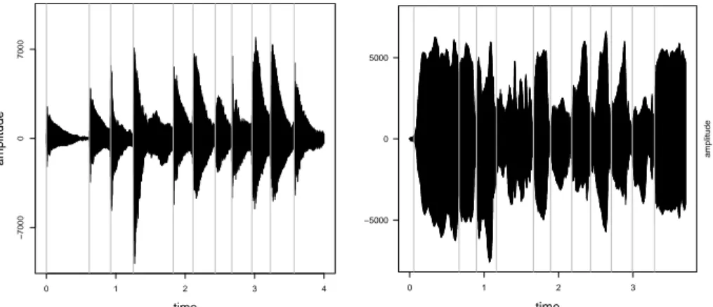
The aim of onset detection (OD) is to recognize the time points of the beginnings of new musical tones. Figure 1 shows the amplitude of the same tone sequence played by piano (left plot) and flute (right plot), respectively. The onset times are marked by vertical lines. This figure illustrates that depending on the music instrument different signal features might to be sensible for OD task. At first, the classical OD algorithm is briefly introduced. Next, the goodness measures of OD and the data sets used for optimization are discussed.

Finally, some details regarding the application of the proposed MBO to OD are provided.

2In [5] we compared 99% and 95% prediction intervals. The 95% prediction interval led to more as “bad” classified points. As better results were achieved with the 99% prediction interval, we propose to use this interval here.

0 1 2 3 4

time amplitude −700007000

0 1 2 3

time

amplitude

−5000 0 5000

Figure 1: Amplitude of the same tone sequence played by piano (left) and flute (right). The vertical lines mark the true tone onset times.

4.1. Onset detection algorithm

The classical onset detection approach is presented in Figure 2 (see, e.g., [7, 21, 10, 5]). In each step, many algorithm parameters are defined which have to be optimized in the experimental part of this work. The considered ranges for the parameter values are discussed at the end of this section.

Figure 2: Eight steps of the classical onset detection approach. Each step has a several parameters to optimize which are given in parantheses.

There are two kinds of onset detection: online and offline. For online OD – in contrast to offline OD – no future signal information is allowed for distinguishing between ‘onset’ and ‘no onset’ in a current signal frame. We assume a digital audio signal sampled with a rate ofFs= 44.1 kHz. This signal is split in the first step intol (overlapping) windows (or frames) of length N samples. If required

by the used OD feature, a Short-Time Fourier Transformation (STFT, [22]) is applied in each signal frame:

Xstft[n, µ] = 1 N

N

X

k=1

xsig[h·(n−1) +k]wN(k)e^−2πiµk/N, (1) wherex_sigis the music signal andX_stft[n, µ] is the Fourier coefficient (a complex number) of the µth frequency bin in nth frame, n = 1, . . . , l. The hop size parameterh determines the distance in samples between the windows. w_N() is the window function (parameterwindow.fun for optimization) which is used to weight the signal amplitude in the frames. See [23] for an overview of such functions.

In the second step, the output of the STFT can be optionally modified.

According to [21] we apply spectral filtering and logarithmize the spectral mag- nitudes. Hence, pre-processing is used only for spectral based OD featured.

For spectral filtering (parameter spec.filt) a filter bank is applied to the spec- tral magnitudes (absolute values of the Fourier coefficients) which bounds the frequency bins according to the semitones of the western music scale:

|Xfilt[n, ν]|=

N/2

X

j=1

|Xstft[n, µ]| ·F[µ, ν]. (2)

Spectral filtering reduces the number of frequency bins for the subsequent fea- ture calculation.

Furthermore, the (optionally filtered) spectral coefficients can be logarith- mized (parameterspec.log in step 3):

|X^log[n, ν]|= log₁₀(`|Xstft[n, ν]|+ 1) (3) where`is a compression parameter.

The computation of an onset detection function in a window of the pre- processed signal is often called reduction (step 4), since after this step not the signal is analyzed anymore but only the ODF values. Many ODFs are based on the comparison of neighboring windows. An increase of an ODF generally indicates a tone onset, a decrease a tone offset. However, also offset information can improve onset detection (see [24]). The algorithm parameterod.fun has 18 levels corresponding to 18 ODFs considered here. These ODF’s are based on the following signal features, some of them use tone offset information: zero-crossing rate, absolute maximum [25], amplitude energy, weighted spectral energy [26], spectral centroid [27], spectral spread [27], spectral skewness [27], spectral flux [7, 8], spectral Euclidean distance [28], phase deviation [29, 8] and complex domain [8]. For example, one of the most popular OD features – spectral flux – is defined as follows:

Spec.Flux(n) =

N/2

X

j=1

H(|X[n, ν]| − |X[n−1, ν]|), (4)

where H(x) = (x+|x|)/2 is a filter which sets the decrease of the spectral magnitude in a frequency bin to zero.

The aim of the normalization (step 5) is to transform theodf feature vector into a standardized form for the subsequent thresholding. At first, exponential smoothing with parameter α can be applied, where forα= 1 the time series stays unchanged and forα= 0 all values of a feature are equal:

sm.odf₁=odf₁,

sm.odf_n=α·odf_n+ (1−α)·sm.odf_n−1. (5) Moreover, for offline OD the normalization of sm.odf is meaningful utilizing e.g., the maximum of theodf feature vector.

Since not every local maximum of an ODF represents an onset, the threshold function aims at the distinction between relevant and non-relevant peaks (step 6). A fixed value for the threshold is unfavorable since the method could then not react to dynamic changes of the signal. Instead, moving threshold functions are widespread [10]:

Tn=δ+λ·mov.fun(|sm.odf_n−lT|, . . . ,|sm.odf_n+rT|),

where the parametermov.fun (moving function) is either the ‘median’, ‘mean’

or ‘p-quantile’. l_T and r_T are the numbers of windows to the left and to the right, respectively, of thenth window.

In the following step the tone onsets are localized in the windows where sm.odf values exceed the threshold and are a local maximum of a certain window sequence (step 7). Following [21] we also use a third condition: A minimum distancemin.dist (in number of windows) between the actual window and the window of the previous tone onsetiprev.onset should be exceeded. To summarize:

O_n=











1, if sm.odf_n > Tn and sm.odf_n= max(sm.odf_n−l

O, . . . ,sm.odf_n+r

O) and n > nprev.onset+min.dist,

0, otherwise.

O= (O₁, . . . , O_l)^T is the tone onset vector andl_Oandr_Oare additional param- eters, namely the number of windows to the left or right of the actual window, respectively, which define the region for local maxima. The left limits of signal frames withO_n= 1 are taken as the time points of the tone onsets.

In [21], it is proposed to report the onsets one window later as actually detected. The authors argue that some features can increase earlier than a human listener would firstly recognize and note a tone onset. For the window length used in [21] this would correspond to a fix time shift of 10 ms. In our work we will consider the parameteronset.shift for optimization (step 8).

In contrast to the most papers on the topic, we do not fix window length N and hop size h a priori but optimize them. This means, that parameter settings corresponding to the number of windows (likerT) could stand for very

different time periods depending onN and h. Therefore, all such parameters are re-defined according to the desired time length,N and h. Hence, we will not consider the parametersrT, lT,rO, lO, andmin.dist, but the timest(rT), t(lT),t(rO),t(lO), andt(min.dist).

In what follows, the regions of interests for all parameter are defined. We will considerN = 512,1024,2048 and 4096 samples as frame length (powers of 2 are chosen in order to apply the fast Fourier transform ). The hop size h lies between N/10 andN. The following window functions are considered for window.fun: ‘Uniform’, ‘Hamming’, ‘Blackmann’ and ‘Gauss’ (with standard deviation σ = 0.4). Parameters spec.filt and spec.log have two settings ‘yes’

and ‘no’. Furthermore,`∈[0.01,20] and the smoothing parameterαvaries in [0,1]. Regarding the thresholding, we optimize δ∈[0,10] and λ∈[1.1,2.6] for mov.fun = ‘median’ or ‘mean’ and fixλto 1 while optimizingp∈[0.8,0.98] for mov.fun = ‘p-quantile’. The shifting parameter onset.shift lies in [−0.01,0.02]

s. Negative values are allowed as it can not be excluded that some features report tone onsets with a certain time delay. For online applications,t(rO) and t(rT) are set to 0 s. In the offline case and universally fort(lO) andt(lT) these intervals are set to [0, 0.5] s. The region of interest for the parametert(min.dist) is [0,0.05] s.

To summarize, there are two application problems to optimize: online and offline OD. Offline OD has a set of 17 parameters while for online OD two parameters are fixed to 0 (i.e., 15 parameters remain for the optimization). In both cases four parameters are categorical and the remaining are numerical.

4.2. Goodness measures for onset detection

In the most onset detection related publications the goodness of onset de- tection is measured by theF-measure (e.g., see [8]):

F = 2·TP

2·TP+FP+FN, F ∈[0,1],

whereTP,FP, andFN stand for the number oftrue positive cases,false positive cases, and false negative cases, respectively, and F = 1 represents an optimal detection. A found tone onset is correctly identified if it is inside a tolerance interval around the true onset. We use here±25 ms as the tolerance [21] while

±50 ms setting is also frequently applied in the literature [7, 8].

Note that thetrue negativecases are not taken into account in the calculation of the F-measure. Another disadvantage is that the distance between true and estimated onsets is only taken into account via the tolerance region. An alternative evaluation measure is therefore the mean (relative) deviation of the estimated onset times from the true ones. This will be called D-measure in what follows. We will optimize theF-measure and use theD-measure only as an additional evaluation feature, e.g., for the clustering in Section 4.4.

4.3. Music data base

The greatest challenge with respect to the creation of a music data base is the necessity of information about the onset times. There are at least two ways to

generate audio data with the corresponding onset times. In the literature, music pieces are manually annotated most of the time, leading to only small numbers of annotated pieces and possible annotation errors. The second possibility is the use of the MIDI format, offering the advantage to have many such music pieces at one’s disposal. There are different programs available which can generate audio recordings in the so-called wave format from MIDI files using instrument specific signal models. Naturally, a music piece generated synthetically in this way will normally not realistically mimic real music recordings.

The aim of the composition of the data base for our optimization is to cover as many music aspects as possible, e.g., way of generation (annotated real music, synthesized MIDI), type of instrument, degree of polyphony, tempo, music genre, and music style. However, it is not meaningful to combine the labeled (real) music pieces with recordings generated from MIDI format as they differ in the onset annotation principle. While for manually annotated pieces the definition of the perceptual tone onset can be applied (i.e., time point where a human listener can firstly recognize a tone onset, [8]), for MIDI pieces the definition of the physical onset is more appropriate (i.e., time point of the first amplitude rise of the new tone, [8]). Hence, we expect that due to delayed annotation in the first case the optimal parameter set can differ from the second case. For this reason, we consider two data bases which will be referred to as WAV and MIDI data sets.

The WAV data base consists of three frequently used manually annotated data sets: data base introduced in [7] with 23 pieces, in [9] with 92 recordings and in [21] with 206 music pieces. Altogether it consists of 2 750 tone onsets.

Many music instruments (like wind or string) and music styles (like European or oriental) are represented in this data set. According to [21], we aggregated true onset times reported within 30 ms to only one tone onset.

The MIDI data base includes the German folk song data base proposed in [28] with 24 music pieces, the MIDI data collection introduced in [5] with 200 pieces and the music epoch data base mentioned in [14] with 22 recordings.

Furthermore, 20 pieces were additionally generated for this work. The most MIDI files were converted to wave files using the MIDI to WAV Converter³ while also theRealConverterproposed in [25] was used. There are overall 63 067 tone onsets in the MIDI data base.

4.4. Onset detection as instance based problem

Although the necessity of parameter optimization arises in nearly all studies on onset detection, they usually just examine a subset of all possible parame- ters, while other parameters are set to some fixed empirical values, which were determined in preview studies or are frequently used in the OD community.

Merely a few numerical parameters are then optimized via grid search or some generic algorithms. This procedure could lead to a local optimum. We aim,

3http://www.maniactools.com/soft/midi_converter/index.shtml.

in contrast, to optimize all parameters simultaneously in order to enable lobal optimization.

The goal of OD optimization is to find the optimal values of the algorithm parameters mentioned in Section 4.1 (inputx) with respect to the meanF-value (outputy). The parameter spaceX of the offline onset detection problem is the Cartesian product of the regions of interest of d = 17 parameters introduced above (in the online case: d = 15). For each problem instance (music piece) the target functionf :X ⊂R^d1×N^d20 →[0,1] is defined as the F-value of the associated OD algorithm (characterized by a point x ∈ X) for this instance, whered1 ansd2 are the numbers of the numerical and the categorical param- eters, respectively. The levels of the categorical parameters are coded with integer numbers (e.g., levels of the parameterwindow.fun are coded as follows:

0 = ‘Uniform’,1 = ‘Hamming’,2 = ‘Blackmann’ and 3 = ‘Gauss’).

For the classical MBO approach the OD performance in xis the averaged F-value over the considered data base ofkmusic piecesI= (I1, . . . , Ik): f(x) = 1/kPk

j=1f(x, Ij). As theF-value has to be maximized, we will minimize the negatedF-value.

With respect to Algorithm 2 more details have to by clarified regarding the OD application. The same surrogate model and infill criterion as mentioned in Section 2 for the classical MBO are used. Although an instance based prob- lem is given, the target variable is defined as the mean performance over all instances (real performance values for “good” points and estimated values for

“bad” points), so that the usual Kriging model and expected improvement cri- terion can be applied. Categorical parameters are transformed into numeric or dummy variables according to the applied approach (naive or dummy Kriging).

In line 3 all instances should be clustered in k_pretest clusters. In [5] we used only the individual F-values of instances in the initial design as classification features. Here, we extend this step by considering also the individualD-values (see Section 4.2). Instances in the same cluster should have similar responses (F- and D-values) for most parameter configurations. In this way we strive to reach the greatest diversity of the music pieces in this pretest subset. The k-means algorithm [30] is used as the clustering approach in line 3.

The size of the pretest subset (kpretest) is set to 5% of the training data volume. This corresponds to 10 pieces for the WAV data set and 8 pieces for the MIDI data set (as in the training phase only 2/3 of the whole data set is used, s. Section 5).

5. Research questions and experimental design

The following main research questions will be studied in this work which can be divided in two classes: optimization questions (OQ) and application questions (AQ):

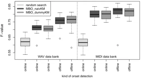
• OQ1: Which surrogate model results in better optimization performance:

naive or dummy Kriging? (Section 2.3)

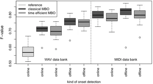
• OQ2: Does the proposed MBO for instance based problems achieve the same values of the target function as the classical MBO, despite the fewer number of function evaluations? (Sections 2 and 3)

• AQ1: Is there a difference in performance between online and offline OD?

(Section 4.1)

• AQ2: Is there a difference in performance between WAV and MIDI data?

(Section 4.3)

This results in 2⁴= 16 ‘optimization strategy - application problem‘ combi- nations. In order to show the efficiency of MBO, a random search with the same number of function evaluations (generated via an LHS design) is also conducted for online onset detection. Furthermore, a simple reference strategy for the pro- posed MBO is also implemented: after the evaluation of the sequential design the optimization in sequential steps is done merely on the kpretest randomly chosen instances.

A very important aspect when comparing many optimization strategies is dealing with over-fitting to the training data. In order to avoid a very good fit on the training data and a much worse performance on new test data, it is essential to use the resampling technique [31]. The most simple resampling technique is the holdout approach where a part of the data (usually 2/3) is used for training and the remaining part for testing. Very popular is thek-fold-cross- validation procedure: Split the data ink disjunct blocks of equal size, conduct the optimization procedure on the training data of k−1 blocks and validate the best found parameter setting on the remaining block (test data). In this manner,kgoodness values (i.e., for each test part) are produced which either can be analyzed as a vector or averaged to only one measure. In the former case two competitive approaches can be compared according to the distribution of the goodness values. As remarked in [32], thekgoodness values are not independent through the block structure of the cross-validation. However, independence is assumed in almost all statistical test.

In order to achieve the independence mentioned above, we replicate the holdout approach 30 times and get, hence, for each optimization strategy a vector of 30 goodness values. In our case, the training data set is used for finding the optimal parameter set of the online or offline OD algorithm while this setting is then applied to the test data. The meanF-value over the music pieces of the test data is then the goodness value of the applied optimization strategy in the respective holdout-replication. In one replication of the holdout approach the same initial design is used for all strategies in order to ensure uniform starting conditions.

As the F-values are not assumed to be normally distributed, the Wilcoxon signed rank test [33, p. 128 ff.] is considered as a non-parametric alternative to the t-test. In accordance with [33] (p. 132) the sample size of 30 observations is sufficient for the desired asymptotic property of the test statistics. Note that although a multiple testing problem occurs here (as some samples have to be applied for testing several times) we waive the methods for holding the global