A Simulation Based Approach to Solve A Specific Type of Chance Constrained Optimization

A Simulation Based Approach to Solve A Specific Type of Chance Constrained Optimization

Lijian Chen

Department of MIS, Operations Management, and Decision Sciences, University of Dayton¹

Abstract: We solve the chance constrained optimization with convex feasible set through approximating the chance constraint by another convex smooth function. The approximation is based on the numerical properties of the Bernstein polynomial that is capable of effectively controlling the approximation error for both function value and gradient. Thus we adopt a first-order algorithm to reach a satisfactory solution which is expected to be optimal. When the explicit expression of joint distribution is not available, we then use Monte Carlo approach to numerically evaluate the chance constraint to obtain an optimal solution by probability. Numerical results for known problem instances are presented.

Keywords: Chance constrained optimization, Monte Carlo, Convex opti- mization

1. Introduction

In health care, supply chain management, and many other industries, the decision makers demand a technique to guarantee the service level under uncer- tainties. For example, hospitals need to ensure that 95% or more patients are seen by a doctor within a short period of time; power planners require power transmission systems to function reliably with almost zero chance of blackout;

suppliers need sufficient network capacity to ensure the successful transportation of goods with a chance of over 90%. A deterministic mathematical programming problem is

min{f0(x) :fi(x)≤0, i= 1, . . . , m, x∈Rⁿ}.

LetI denote a set of indicesi such that the constraint fi(x)≤0 was contam- inated with random vectorξ : Ω→R^s of a probability space (Ω,B,P). These constraintsfi(x, ξ)≤0, i∈I, as a whole, represent an event which demands se- rious attention of the decision makers. This event was desirable but not required almost surely. Thus, we impose a probabilistic measure

P{fi(x, ξ)≤0, i∈I} ≥1−α

1300 College Park Ave, Dayton, OH 45469, Tel.: +1-937-229-2757,lchen1@udayton.edu

to represent the fact that decision makers may need this desired event by the chance of 1−α, at least. The model becomes

min{f0(x) :fj(x)≤0, j /∈I,P{fi(x, ξ)≤0, i∈I} ≥1−α}.

Chance-constrained optimization has little progress made until recently due to its complexity. It may be the case that the only way to check the feasibility of a given point is to use Monte Carlo simulation. To calculate the joint cumulative distribution function explicitly, we also need considerable investment on com- puters. In addition, the feasible set can be non-convex even iffi(x, ξ), i∈Iare linear with respect tox. Thus, the research on the chance-constrained optimiza- tion has gone into two somewhat different directions. One is to transform the original problem into a combinatorial problem such as [6] through discretizing the probability distribution. Another is to approximate the chance constraint by a convex function to extract function value and gradient. The obtained solu- tions are mostly satisfactory but sub-optimal. These solutions seem to be very practical and reasonable for certain problem instances. However, the heuris- tics solution may raise the concern of the solution quality due to lack of either functional or probabilistic linkage to the true optimal solution.

In this paper, we only investigate a specific type of chance-constrained opti- mization in which the random vector appears in the right-hand side of the affine mapping and the distribution ofξ is jointly continuous, and log-concave. The reason that we impose these conditions is to equivalently transform model (1) to a convex optimization. This reason is based on the following results from the literature.

Theorem 1. If ξ ∈ R^m is a random vector that has log-concave probability distribution, then the function

Fξ(Dx) :=P{Dx≥ξ}

is log-concave with respect to x. D ∈ R^m×n is a real matrix of coefficients.

Moreover, the set

{x∈Rⁿ:P(Dx≥ξ)≥1−α}

is convex and closed.

The proof is in [11, Chapter 5].

In business analytics, the decision is usually subject to multiple resource constraints. We impose a joint probability measure on a handful of constraints to ensure a 1−αchance of realization. We have

minf0(x)

Subject to:fj(x)≤0, j /∈I (Resource constraints) P(Dx≥ξ)≥1−α, x∈Rⁿ (Chance constraint) where the distribution ofξis joint log-concave and continuous and D is deter- ministic. Therefore, the above has a convex and closed feasible set. Let

g(x) := log(1−α)−log(Fξ(Dx))≤0

whereFξis the cumulative distribution function of the random vectorξ. g(x) is a convex function with respect tox∈Rⁿand the chance-constrained optimization model is equivalent to

minf0(x)

subject to: g(x)≤0 (CCCF)

fi(x)≤0, i /∈I

If other constraints, f0(x), fi(x), i /∈ I, are convex, model (CCCF) is a con- vex optimization problem. The term CCCF stands for a Chance Constrained problem with Convex Feasible set. We are not endorsing the superiority of convex modeling but emphasizing the fact that the convex optimization will always yield global and reliable solutions. Moreover, the convex optimization with smooth constraints will always terminate within a polynomial number of iterations without acquiring the second-order information (see [8, Chapter 2]).

The key contribution of this research is to approximate the functional value, g(x), and gradient,∇g(x), by a Bernstein polynomial-based function. First, the Bernstein polynomial can effectively control the approximation errors of function values and gradients simultaneously. Second, the degree of polynomial can be well-controlled by Jackson’s theorem V (see [1]). Third, our approximation will preserve the convexity and the differentiability ofg(x). The log-concave assump- tion will be less likely to become a serious obstacle of implementation because many commonly-used distributions are indeed continuous and log-concave. For instance, uniform distribution, normal distribution, beta distribution, Dirich- let distribution, Pareto distribution, and gamma distribution (when the shape parameter is greater than one) are continuous and log-concave.

We need to show another primary reason that we adopt the Bernstein poly- nomial in this research. One may argue that there are many routes to approxi- mate such a chance constraint and we agree. We have no intention to endorse our approach over another approximation scheme developed in parallel. How- ever, given the fact that g(x) is convex, our approximation is mathematically guaranteed to be convex and, at the same time, our approximation will stay within an error range uniformly. In particular, we need not only the functional value but also the gradient. It is always a good idea to approximate a convex function with another convex function when both function and its first-order information are extracted. In comparison to a non-convex approximation to the original function, a convex approximation has no local zigzag fluctuations which may considerably affect the approximation of the first-order information such as gradient or sub-gradient. A guaranteed convex function will ensure very limited complication when evaluating the gradient.

The remainder of this paper is organized as follows. The approximation approach is described in Section 2, beginning with reasoning and details followed by the approximation procedure. In Section 3, we describe our approach for the chance-constrained optimization along with the computational complexity. In Section 4, we discuss the impact of using Monte Carlo to evaluate the cumulative distribution function. We also show that the obtained optimal solution, if Monte

Carlo is adopted, will converge to the original optimal in probability. In Section 5, we present the spreadsheet-based implementation which is a combination of business analytic and convex optimization solvers. We conclude this paper in Section 6 with concluding remarks about this new approach.

2. A polynomial approximation approach

In order to highlight the approximation approach, we further relax the non- linear smooth but convex constraints with linear functions.

minc^′x

subject to:g(x)≤0 (CCCFL)

Ax≤b, x∈Rⁿ

where c represents the coefficients for the objective function. The new set of constraints, Ax ≤b, is in the place of the resource constraints fj(x) ≤0, i /∈ I. We name this problem the Chance Constrained optimization with Convex Feasible set and Linear resource constraints (CCCFL).

The functiong(x) is defined onRⁿ ontoR. Thus, the value ofg(x) will be a scalar and the gradient∇g(x) is an-dimensional vector. Thei^th component is ∂g(x)

∂xⁱ , x := [x¹;. . .;xⁿ] where xⁱ represents the ith component of x, i.e.

∇g(x) = ∂g(x)

∂x¹ ;. . .;∂g(x)

∂xⁿ

. Let us define thei^th marginal function ofg(x) as gi(xⁱ) : [aⁱ, bⁱ]→Rwith respect to xⁱ ∈[aⁱ, bⁱ] and other componentx^j, j 6=i fixed. We would evaluate ∂g(x)

∂xⁱ by calculating the derivative of the marginal functiongi(xⁱ) that ∂g(x)

∂xⁱ =∇gi(xⁱ). Sinceg(x) is convex, all of its marginal functions gi(xⁱ), i = 1, . . . , n are convex with respect to xⁱ. Our approach is to approximate all the marginal functions ofgi(xⁱ) with convex, differentiable polynomial of degreek,qk(xⁱ) at a fixedx. We use the vector [q_k^′(x¹);. . .;q_k^′(xⁿ)]

to estimate∇g(x).

We show the construction of qk(xⁱ) to approximate the marginal function gi(xⁱ) : [aⁱ, bⁱ]→R. This idea is inspired by the Weierstrass theorem that any continuous function can be approximated by a polynomial with adequately large number of order. However, the choice of proper polynomial will considerably affect the approximation performance. In this research, we adopt a polynomial named Bernstein polynomial:

Definition 1. The Bernstein polynomial of functionφ(y)∈C¹[0,1]is Bk(φ;y) =

k

X

j=0

k j

y^j(1−y)^k−jφ(j/k) for anyk= 0,1,2, . . ..

For the sake of simplifying notations, we useφ(y) in the place ofgi(xⁱ). Without loss of generality, we assume thatφ(y) is on [0,1] as we can always scale a 1-1 mapping from a closed interval [aⁱ, bⁱ] to [0,1]. There is a theorem associated with the Bernstein polynomial.

Theorem 2 (Voronovskaja theorem). If φ(y) is bounded on [0,1], differ- entiable in some neighborhood of y and has second derivative φ^′′(y) for some y∈[0,1], then

klim→∞k|φ(y)−Bk(φ;y)|= y(1−y) 2 φ^′′(y).

Ifφ(y)∈C²[0,1], the convergence is uniform.

The proof of this theorem is in many papers such as [9]. This theorem states that the value ofBk(φ;y)−φ(y) tends to zero at the speed of 1

k wherekrepresents the degree of the approximating Bernstein polynomial. That is, any smooth function would be approximated by Bernstein polynomial of degreek with ar- bitrary accuracy as k→ ∞. Nevertheless, the approximation using Bernstein polynomial is rather poor because, to halve the error, we have to increase the degree fromk to 2k. In order to improve the approximation performance, we can use Bernstein polynomial to approximate the second order derivate of the original function which is based on the following result.

Theorem 3. There exists a sequence of component functions,

ψ0(y), ψ1(y), ψ2(y). . . , (1) each convex on [a, b], such that any convex function φ(y) ∈ C¹[a, b] may be approximated with arbitrary accuracy on[a, b]by a sum of non-negative multiples of the component functions.

This theorem is extremely important to our research, and we present it here as a courtesy from the original source.

Proof: It will be adequate to show this conclusion on [0,1] because we can make a linear change of variable, if necessary, to transform any finite interval [a, b] onto [0,1]. Let us suppose that we wish to approximate to a given convex functionφ(y)∈C¹[0,1]. At first, by Votonovskaja theorem, it is valid to assume thatφ(y) is continuously twice differentiable. We use the Bernstein polynomials indirectly and write

Bk(φ^′′;y) =

k

X

j=0

k j

y^j(1−y)^k−jφ^′′(j/k) (2) Let us observe that y^j(1−y)^k−j ≥ 0 on [0,1] and that in (2) φ^′′(y) is being approximated by a sum of non-negative multiples of the polynomialy^j(1−y)^k−j.

Fork≥2, defineqk(y) by

q^′′_k(y) =Bk−2(φ^′′;y); q_k^′(0) =φ^′(0); qk(0) =φ(0) (3)

We see thatqk(y) is a polynomial of degree at mostk. We also defineβj,k(y), for 2≤j≤k, by

β_j,k^′′ (y) =y^j−2(1−y)^k−j; β_j,k^′ (0) =βj,k(0) = 0 (4) To complete the definition of the polynomialsβj,k(y), we define,

β0,k(y) =sign[φ(0)]; β1,k(y) =y×sign[φ^′(0)] (5) The relevance of the choice of function (5) will be seen later. We then have that

qk(y) =

k

X

j=0

cjβj,k(y) (6)

cj ≥0 andβ_j,k^′′ (y)≥0 on [0,1]. Now, given any ǫ >0, there exists an integerk for which

|Bk−2(φ^′′;y)−φ^′′(y)|< ǫ, |q_k^′′(y)−φ^′′(y)|< ǫ (7) on [0,1] and therefore, fory∈[0,1],

Z y

0

(q_k^′′(t)−φ^′′(t))dt

≤ Z y

0

|q^′′_k(t)−φ^′′(t)|dt≤ǫy≤ǫ (8) Using (3), the inequality (8) give

|q^′_k(y)−φ^′(y)|< ǫand |qk(y)−φ(y)|< ǫ (9) Recalling the definition of qk(y) in (6), we see that this last inequality (9) completes the proof for case whenφ^′′(y) exists. Note that the polynomialβj,k(y) may be enumerated asψ0(y), ψ1(y), ψ2(y), . . ..

We highlight key results here. First, the inequality (9) shows that our ap- proach is capable of controlling the approximation errors of φ(y) and φ^′(y) simultaneously. In comparison to our approach, a general polynomial approx- imation by Weierstrass theorem can only approximate arbitrarily close to the function rather than both function and gradient at the same time. Second, we can always numerically consider any convex function on [0,1] to be continuously twice differentiable. This property is very important to our research that we can always assume high-order differentiability of g(x). Otherwise, we can al- ways construct a higher-order Bernstein polynomial which approximateg(x) to within ǫ

2 on [0,1] to ensure (9).

We now address the choice of the non-negative coefficients cj. From the previous analysis, we set

ψj(y) =βj,k(y),2≤j≤k

ψ0(y) =sign[φ(0)] (10)

ψ1(y) =y×sign[φ^′(0)]

and the polynomialsβj,k(y) are easily computed because forj ≥2, β_j,k^′′ (y) =y^j−2(1−y)^k−j =y^j−2

k−j

X

ℓ=0

(−1)^ℓ k−j

ℓ

y^ℓ. (11) Thus,

βj,k(y) =y^j

k−j

X

ℓ=0

(−1)^ℓ k−j

ℓ

y^ℓ

[(ℓ+j)(ℓ+j−1)] (12)

We construct

qk(y) =

k

X

j=0

cjψj(y).

The value ofcj are determined minc

s=1,...,k+1max {φ(ys)−

k

X

j=0

cjψj(ys)}: cj≥0

(13) In the above model, we takek+1 observations on [0,1], (ys, φ(ys)), s= 1, . . . , k+

1 whereysare predetermined values on [0,1]. This model is a convex optimiza- tion problem withk+1 variables and its computational complexity isO((k+1)³) at the worst case (see [3]). The approximation constructed by (13) is named thebest approximation orleast square approximation (see [4]).

In addition, we still need to determine the choices on the degree ofkand the correspondingk+ 1 points, i.e., (ys, φ(ys)), s= 1, . . . , k+ 1. By theorem 3, the approximation error can be controlled by increasing k. However, in practice, high-degree polynomials usually cause Runge’s phenomenon (see [9]), which means that the approximation is extremely unstable. The primary cause of Runge’s phenomenon is due to the polynomial of high degree such as a degree of 1,000 or more. The following theorem addresses the issue that the Runge’s phenomenon is less of a concern to our approach because we only need a low- degree polynomial.

Theorem 4 (Jackson’s theorem). Ifφ(y)isr-differentiable ony∈[0,1]and φ(y) is approximated by the best approximation qk(y) of degree k (constructed by theorem (13)), then the approximate error ofφ(y)on[0,1]byqk(y)satisfies,

ymax∈[0,1]|φ(y)−qk(y)| ≤ π

2 r

|φ^r(ω)|

[(k−r+ 2). . .(k)(k+ 1)], k≥r

where φ^r(ω) represents the r-order derivative of φ(y) at some ω ∈ [0,1] and ys, s= 1, . . . , k+ 1 are distinct predetermined points on[0,1].

This is called Jackson’s Theorem V introduced in [4, Page 147]. The derivation of the theorem is very lengthy and technical. We now present the history and the outline of this theorem and its impact to our approach. In 1911, D. Jackson presents the first Jackson’s theorem as follows:

Theorem 5. Given f(x) is a continuous function with a period 2π, has r-th derivative (r >1), and satisfies the inequality

|f^(r)(x)| ≤1.

Then, there exists for any positive integer n a trigonometric sum Pn−1(x) of order less thann and this trigonometric sum satisfies the inequality

|f(x)−Pn−1(x)| ≤ Ar

n^r,0≤x≤2π, and hence the value ofAr depends solely on the value ofr.

This theorem is later published in [7]. Essentially, this theorem states that the approximate error is bounded and the reduction on error is extremely fast as we increase the degree of the approximate polynomial. Next, every even trigono- metric polynomial can be expressed as an algebraic polynomial and conversely.

Hence, the error in the best approximation bytrigonometric polynomial is the same as the error in the best approximation byalgebraic polynomials.

Jackson’s Theorem V is extremely important result supporting our approach.

In theory, it shows that if we approximate ar-differentiable function by algebraic polynomials, the error will be fast reduced by increasing the order of polyno- mial. Thus, Runge’s phenomenon is less of a concern because the approximate polynomial of a very limited degree would be adequate to control the approxi- mation error. We need to remark that the assumption ofr-differentiableφ(y) can be justified by the Voronovskaja theorem. Although we find the coverage of the differentiability of probability functions in [12, Section 4.4.1], we need to justify ther-differentiability withr >1. The argument is that ifφ(y) is indeed r- differentiable, we can apply the theorem directly. Otherwise, we need to ap- ply the Voronovskaja theorem as long as the original function is convex. We can always find a smooth approximation constructed by Bernstein polynomial which isr-differentiable. Moreover, the value ofφ^r(ω) is well bounded in a close and bounded interval with a predeterminedrbecause of the similar argument suggested by the Voronovskaja theorem.

We need to adopt the Chebyshev nodes on [0,1] to select k+ 1 distinct points (ys, φ(ys)), s= 1, . . . , k+ 1 to control the error, maxy∈[0,1]|φ(y)−qk(y)|.

Although Jackson’s Theorem guarantees to bound the error, a good selection of (ys, φ(ys)), s= 1, . . . , k+ 1 will greatly reduce the error (see [13, Lecture 20]) in practice. When we interpolatingφ(y) at point (ys, φ(ys)), s= 1, . . . , k+ 1, the error is

ymax∈[0,1]|φ(y)−qk(y)|= Π^k+1_s=1(y−ys) φ^k(ω)

(k+ 1)! (14)

The term Π^k+1_s=1(y−ys) needs to be minimized and thus we adopt the Chebyshev nodes. TheChebyshev nodes on [0,1] which are described as follows.

ys:=1 2 −1

2cos

2s−1 2k+ 2π

, s= 1, . . . , k+ 1

When Chebyshev nodes are implemented, Π^k+1_s=1(y−ys) will be minimized to 1 2^k and if we assume that|φ^k(y)| ≤M, we have

ymax∈[0,1]|φ(y)−qk(y)| ≤ 1

2^k(k+ 1)!M. (15)

At a given error boundǫ >0 forg(x), we need to control the error of everyφ(y) no greater than ǫ

n. Thus, the necessary degree ofqk(y) should be min

k: 1

2^k(k+ 1)!M < ǫ n

(16) Increasing the degree ofqk(y) fromktok+1 means a reduction of approximation error by 2(k+ 1), which is extremely fast. Askkeeps growing, the reduction of error will be much faster. Thus, it is extremely unlikely that our approximation approach will require high-degree polynomials. For example, n = 20, M =

kvalues k= 5 k= 6 k= 7 k=8 k= 9 k= 10

n

2^k(k+ 1)!M 0.0868 0.0062 3.87×10⁻⁴ 2.15×10⁻⁵ 1.07×10⁻⁶ 4.89×10⁻⁸ Error reduction 100% 7.1429% 0.4459% 0.0248% 0.0012$ 0.0001%

Table 1: Extremely fast convergence by degree of approximating polynomial

100, ǫ= 10⁻⁴, we present the values of n

2^k(k+ 1)!M by distinct degrees in table 1. We also take the error bound of degreek = 5 as the baseline and present the relative precentage of error with greater degrees to demonstrate the fast reduction in the approximate error. With such a fast rate of error reduction, our approach will not suffer the Runge’s phenomenon at all.

There are many approximate approaches being developed in parallel. We have neither intention nor interest to show the superiority against all the ap- proximation approaches. However, our approach does outperform the approx- imation of some other polynomial of degree k. For example, 1, y, y², . . . , y^k, the approximation function may fail to preserve convexity and the performance of evaluating gradient is poor. Let qk(y) denote the approximation function of our approach and ¯qk(y) represent the approximation function constructed from 1, y, y², . . . , y^k rather than polynomial (10). In Table 2, wheny = 0, y = 0.2, y = 0.7 and y = 1.0, the gradients of our approximation functions con- siderably outperform their counterparts constructed from 1, y, y², . . . , y^k. The poor performance of ¯qk(y) is because the error control will be valid only for the function value and there is no control on its gradient.

We present the procedure to estimate ∇φ(y) where φ(y) ∈ C¹[0,1] by a polynomialqk(y).

Step 1. Determine the overall error boundǫ >0.

Step 2. Choose the degreek≥10.

y φ(y) q¯k(y) qk(y) ∇φ(y) ∇q¯k(y) ∇qk(y) 0.0 1.000 0.996 0.992 -3.14 -3.54 -3.16 0.2 0.412 0.411 0.410 -2.54 -2.37 -2.48 0.4 0.049 0.063 0.058 -0.97 -1.01 -0.94 0.7 0.191 0.189 0.195 1.85 1.92 1.83 0.9 0.691 0.718 0.702 2.99 3.07 3.08 1.0 1.000 1.012 1.023 3.14 2.65 3.28

Table 2: A comparison of the approximations of the function 1−sinπy, y∈[0,1].

Step 3. Calculatek+ 1 coordinates, (ys, φ(ys)), s= 1, . . . , k+ 1 which are de- termined as Chebyshev nodes on [0,1].

Step 4. Solve (13) and constructqk(y).

Step 5. Useq_k^′(y) as an approximation ofφ^′(y).

3. Computational complexity

The overall computational performance is also determined by the choice of the main algorithm. In this research, we adopt the gradient mapping method in [8] as our primary algorithm for two reasons: first, this method terminates within a polynomial number of iterations, second, only the first order information such as functional value and gradient are required. We cite the results from [8] as the foundation of our complexity analysis and we refer readers to that book for more technical details.

We now present the number of arithmetic operations including additions, multiplications, divisions, and comparisons for our approach to show that our approach leads to the optimal solution at a cost of polynomial complexity. First, we show the computational complexity of evaluatingg(x) and∇g(x) at a given x. Second, we present the overall complexity with a first-order method as the main algorithm. In this analysis, there are a few required parameters includ- ing the significance levelα; the degree of the approximation polynomialk; the dimension of x, n; and the overall accuracy, ǫ > 0. We must remark that the arithmetic operation count is a measure of computational complexity which ignores the fact that adding or multiplying large integers or high-precision float- ing point numbers is more demanding than adding or multiplying single-digit integers.

Proposition 1. If the number of arithmetic operations to evaluate gi(xⁱ_s) is bounded by a fixed value P, to construct model (13), it requires up to (k+ 1)²O(k) + (k+ 1)P arithmetic operations.

Proof: Model (13) needsk+ 1 times ofgi(xⁱ_s), s= 1, . . . , k+ 1 which takes (k+ 1)P. The construction of polynomial will need to calculateψ0(xⁱ), . . . , ψk(xⁱ).

Since these terms are simple polynomials and each one of their calculations only takes up toC×karithmetic operations whereCis a large constant, we thereby

consider that each term will take up to O(k) arithmetic operations regardless trivial differences among them. Thus, in order to calculateψ0(xⁱ), . . . , ψk(xⁱ), which means k+ 1 times of O(k) arithmetic operations for each item s, s = 1, . . . k+ 1. Thus, we need up to (k+ 1)²O(k) + (k+ 1)P arithmetic operations

to construct model (13).

Model (13) has k+ 1 variables and the number of arithmetic operations required isO[(k+ 1)³]. Thus, we need

n{O[(k+ 1)³] + (k+ 1)²O(k) + (k+ 1)P}

arithmetic operations to obtain the approximates of g(x) and ∇g(x). Since the calculation of derivatives of the polynomial is “transparent”, the number of operations will be trivial and not cause any computational concerns.

By adopting the gradient mapping method in [8], we have the following result,

Proposition 2. The gradient mapping method takes at most 1

ln[2(1−κ)]ln t0−t^∗

(1−κ)ǫ (17)

iterations to obtain anǫ−optimal solution where κis an absolute constant (for exampleκ= 0.25) and t0, t^∗ are the progressively updated penalty coefficients.

The proof is in [8]. In the proof, both κand t0−t^∗ are well bounded values.

Thus, the value of (31) will be bounded as well. In [3], the authors suggest that the number of algorithmic iterations will be as many as 30. Based on this result, we show that

Theorem 6. The overall number of arithmetic operations towards anǫ-optimal solution will be

n{O[(k+ 1)³] + (k+ 1)²O(k) + (k+ 1)P} 1

ln[2(1−κ)]ln t0−t^∗ (1−κ)ǫ when we use the gradient mapping algorithm.

For instance, when we have a chance-constrained optimization withn= 10,000 variables. We choose to approximate this constraint by polynomials withk= 13 degree. Supposeǫ= 0.01,m= 100, κ= 0.25, andt0−t^∗= 100, the number of arithmetic operations should be

10000{O(14³) + 14²O(14) + 14P} 1

ln[2×0.75]ln 100 0.75×0.01.

The overall number of arithmetic operations should be in the level of 1×10¹⁶ arithmetic operations. Modern computers are far more capable of handling such a scale calculation. Recently, Intel Corporation demonstrated a single x86-based desktop processor sustaining more than a Tera-FLOP (10¹²). This means that solving such a large scale chance-constrained optimization problem on an average desktop computer will only take several hours. Our computational performance supports this conclusion.

4. Evaluation of the cumulative distribution function

In the previous sections on the approximation approach and the complexity, it seems that the evaluation ofFξ(x) can be completed easily. In reality, the evaluation ofFξ(x) :=P(Dx ≥ξ) is a great deal of challenges because it is a multivariate integration and computationally demanding. In particular, when the distribution ofξis assumed to be log-concave without a closed-form, explic- itly evaluating Fξ(x) is nearly impossible due to the multivariate integration.

We thus need to adopt Monte Carlo to bypass the multivariate integration. The simulation error can be well controlled and if the result is not satisfactory, we can always increase sample size for an improvement.

Consider an independent and identically distributed (iid) sample with sample sizeN,ξ¹, . . . , ξ^N. Let

F_ξ^N(x) :=

PN

i=1I(ξⁱ ≤Ax)

N (18)

where I(a) = 1 when a0, a∈R^s and I(a) = 0 otherwise. F_ξ^N(x) refers to the estimated cumulative distribution ofξbased on the sampleξ¹, . . . , ξ^N and

g^N(x) := log(1−α)−log PN

i=1I(ξⁱ ≤Ax) N

.

The introduction of Monte Carlo will not complicate the computational com- plexity results. When adopting simulation to evaluateFξ(x), we may have a different number of arithmetic operationsPN rather thanP at a given sample sizeN. It is less of a concern as long as thePN is well bounded andPN is the number of algorithmic operations with respect to a sample size ofN. Thus,PN

is well bounded as long as the values ofP andN are bounded by the problem input. Consider

g_i^N(xⁱ_s) = log(1−α)−log(

PN

j=1I(ξ^j≤D[x¹;. . .;xⁱ⁻¹;xⁱ_s;xⁱ⁺¹;. . .;xⁿ])

N )

whereD ∈R^m×n. For the indicator function, it takes m(n+n−1) additions and multiplication, mcomparisons against the m-dimensional ξ^j, and another mcomparisons with 0. We assume that the calculated values will be properly stored in memory. We need to repeat such a calculation N times with an additionalN additions and divisions to calculate the average. If we count the logarithmic calculation evenly as other arithmetic operations, we need 2 more logarithmic operations and one addition. Thus, the total number of arithmetic operations will be

N(m(n+n−1) +m+m) +N−1 + 1 + 1 + 1 =N(m(2n−1) + 2m) +N+ 2 which is expected to be bounded with predeterminedN andP.

The incorporation of Monte Carlo removes the computationally demanding multivariate integration. However, Monte Carlo complicates the problem that

the obtained optimal solution becomes a random variable. Thus, an ideal result will be that the obtained optimal converges to the true optimal in probability.

We define

X :={x|fj(x)≤0, j /∈I}.

andX is a compact set. The original chance constrained optimization model is min{f0(x)|g(x)≤0, x∈X}. (19) The interim problem, whereg(x) is replaced by the sample averageg^N(x), is

min{f0(x)|g^N(x)≤0, x∈X} (20) and the model we actually solved is:

min{f0(x)|Qk(x)≤0, x∈X} (21) whereQk(x) :Rⁿ→Ris the polynomials of degreekat an aggregated level for allndimensions ofxof the function g^N(x).

Letx^∗, ˆx^∗, and ˆx^∗_kdenote the optimal solutions from (19), (20), and (21), re- spectively. These problems can be written as unconstrained optimization prob- lems:

min f0(x) +tQk(x)+, t >0, x∈X, Qk(x)+:= max{0, Qk(x)} (22) min f0(x) +tg^N(x)+, t >0, x∈X, g^N(x)+ := max{0, g^N(x)} (23) min f0(x) +tg(x)+, t >0, x∈X, g(x)+:= max{0, g(x)} (24) and we have the following theorem for the penalty method.

Theorem 7. Let there exist a value ¯t >0 such that the sets S1={x∈X|f0(x) + ¯tQk(x)+ ≤f0(ˆx^∗_k)}

S2={x∈X|f0(x) + ¯tg^N(x)+≤f0(ˆx^∗)}

S3={x∈X|f0(x) + ¯tg(x)+≤f0(x^∗)}

are bounded. Then

hlim→∞f0(xh) =f0(ˆx^∗_k), lim

h→∞Qk(x)+= 0, xh∈S1 hlim→∞f0(xh) =f0(ˆx^∗), lim

h→∞g^N(x)+= 0, xh∈S2

and

hlim→∞f0(xh) =f0(x^∗), lim

h→∞g(x)+= 0, xh∈S3

wherek represents the degree of polynomial and{xh} is the sequence of points generated by the main algorithm.

The proof is in [8] as a general conclusion for the penalty method and the choice of ¯tis rather theoretical and symbolic. Thus, we define

uk(x) :=f0(x) + ¯tQk(x)+, u(x) =¯ f0(x) + ¯tg^N(x)+, andu(x) =f0(x) + ¯tg(x)+

Consider a sequence of functionsuk :Rⁿ→R. It is said that uk epi-converges to a function ¯uif the epigraphs of the functions uk converge, in a certain set valued sense, to the epigraph of ¯u:Rⁿ →R. In order to establish connection between ˆx^∗_k andx^∗, we need two phases. First, we need to show the convergence from ˆx^∗_kto ˆx^∗and from infuk to inf ¯u. Second, we need to show the convergence at least in probability from ˆx^∗to x^∗.

4.1. Convergences ofxˆ^∗_k toxˆ^∗ andinfuk toinf ¯u

In order to show the convergences of ˆx^∗_k to ˆx^∗ and infuk to inf ¯u, we need the following convergence in minimization theorem (see [10]):

Theorem 8 (convergence in minimization). Suppose the sequence{uk}, i= 1, . . .is eventually level-bounded and{uk}epi-converges tou¯withukandu¯lower semi-continuous and proper. Then

infuk →inf ¯u (25)

while{uk} is indexed over a sub-sequence of Z₊ containing all ν beyond some

¯

ν. The sets argminuk are nonempty and form a bounded sequence with lim sup

k

(argmin uk)⊂argminu.¯ (26) Indeed, for any choice ǫk → 0 and xˆ^∗_k ∈ ǫk-argmin uk, the sequence {ˆx^∗_k} is bounded such that all of its cluster points belong to argmin u. If argmin¯ u¯ consists of a unique pointˆx^∗, one must actually havexˆ^∗_k→xˆ^∗.

The proof is in [10] and this theorem plays a central role to establish the first connection. With a large enough N,g^N(x) is proper, continuous, and level- bounded and so is ¯uin probability. Our approximation approach generates a good approximation, Qk(x), to g^N(x) within a uniformly controlled range of error. Therefore, functionsQk anduk onX should be proper, continuous, and level-bounded as well. When we use the same sample in our approximation approach,g^N(x) is convex and so isQk(x). Whenuk and ¯uare strictly convex, there will beuniqueoptimal solutions ˆx^∗_k and ˆx^∗for (22) and (23), respectively.

If the sequence of functions {uk} epi-converges to {¯u}, we can then apply theorem 8 to establish the convergences of ˆx^∗_k to ˆx^∗ and infuk to inf ¯u. We need to prove the uniform convergence of the sequence of functions{Qk}tog^N because of the following proposition:

Proposition 3. With a large enough N, if {Qk(x)} epi-converges to g^N(x) on X and f0 is continuous on X, then the sequence of functions uk(x) :=

f0(x) + ¯tQk(x)+ epi-converges to u(x) :=¯ f0(x) + ¯tg^N(x)+ for any ¯t > 0 in probability.

Therefore, it is adequate to show that {Qk(x)} epi-converges to g^N(x) on X under a certain sample. We have the proposition that states the epi-convergence from uniform convergence as follows:

Proposition 4. With a large enoughN, consider{Qk(x)}andg^N(x) :X →R, if the functionsQk(x)are continuous on X and converges uniformly tog^N(x) onX, thenQk(x)epi-converges tog^N(x)relative toX in probability.

The above two propositions are proved in [10, Chapter 7]. We complete this phrase by the following theorem

Theorem 9. With a large enough N, the sequence of function {Qk(x)} uni- formly converges tog^N(x)onX in probability.

Proof: SinceQk(x) andg^N(x) are continuous onX, then {Qk(x)} andg^N(x) are bounded. With our approximation approach at any given ǫ > 0, let the sequence of function be indexed with ¯k ≥ min

k : 1

2^k(k+ 1)!M < ǫ n

, we have

|Qk(x)−g^N(x)| ≤ǫfor allx∈X

Thus, we claim that{Qk(x)}uniformly converges tog^N(x)in a bounded sense.

From the above uniform convergence, we can immediately show that{Qk(x)}

epi-converges tog^N(x) onX by applying propositions 3 and 4.

4.2. Convergences ofxˆ^∗ tox^∗ andinf ¯utoinfu

We must remark that ¯uis also a sequence of functions by distinct iid samples with ascending sample size N and let{u¯^N} denote this sequence of functions indexed by the corresponding sample size. Let ˆx^∗_N denote the point which minimizes ¯u^N onX. By the law of large numbers, for ax∈X,

Nlim→∞

P(|u¯^N(x)−u(x)|> ǫ) = 0, or equivalently writing as ¯u^N(x)→pu(x) asN → ∞ (27) which is calledpointwise convergence in probability of random convex functions.

Theorem 10. If the sequence of functions{¯u^N}, atx∈X,u¯^N(x)→pu(x)as N→ ∞ andu¯^N,uare convex onX, then

sup

x∈X

|¯u^N(x)−u(x)| →p0as n→ ∞

Proof: Letx1, x2, . . .be a countable dense set of points inX. Since ¯u^N(x1)→p

u(x1) as N → ∞, there exists a sub-sequence along which convergence holds almost surely. Along this sub-sequence, ¯u^N(x2) →p u(x2) so a further sub- sub-sequence exists along which also ¯u^N(x2)→u(x2) almost surely. Repeating this argument by applying cumulative sub-sequencesktimes, we have ¯u^N(xj)→ u(xj) almost surely forj = 1, . . . , k. Now consider the new sub-sequence formed by taking the first element of the first sequence, the second element of the second,

and so on. Along the new sub-sequence we must have ¯u^N(xj)→u(xj) almost surely. Thus, we have this corollary:

sup

x∈X

|¯u^N(x)−u(x)| →0 almost surely along this sub-sequence.

Therefore, for any sequence, a further sub-sequence can be constructed along which sup_x∈X|¯u^N(x)−u(x)| →0 almost surely which automatically implies

sup

x∈X

|¯u^N(x)−u(x)| →p0 along the whole sequence.

As an immediate result, we have

Corollary 1. Supposeuhas a unique minimum at x^∗∈X. Letxˆ^∗_N minimize

¯

u^N, thenxˆ^∗_N →px^∗ as n→ ∞.

This proof is a simpleǫ−δargument.

Hence, we conclude that the sequence of the solution of (21) uniformly con- verges the optimal solution of (19) in probability.

5. Implementation and sample results

We code our approach to solve model (CCCFL). Software implementation includes five components: the main code, the function to calculate the functional value ofg(x), the function to calculate the gradient ofg(x),∇g(x), the function to calculate the Chebshev nodes, and the software utility to load the model into the compatible format of certain software packages. In our numerical experi- ments, we use the platform of Matlab R2013a with the third-party Disciplined Convex Programming developed by Stanford University. The hardware is a HP workstation running Debian Linux Wheezy with 16G DDR3 memory and Intel i7-4770 CPU. The computational architecture is x86-64 and so do both Matlab and CVX package.

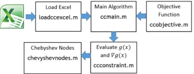
Since the chance constrained optimization problem is commonly used for business planning problems, we design the interface of modeling to be business friendly that we use Microsoft Excel templates to collect and organize the mod- eling parameters. All the parameters such asA, D, b, c, αare worksheets which will be loaded by the software utility. We illustrate the structure of our package in Figure 1. The main code will briefly check the dimensions of the variables and exit if there is a mismatch. If the model is successfully accepted by the main code, you may see the algorithm running until it terminates at the so- lution which satisfies the stopping criterion. We use this package to solve two chance constrained optimization problems in the field of financial planning, and transportation.

Figure 1: Functions of the software package

5.1. Cash matching

We tested our approach along with software packages on the chance-constrained optimization problem named “cash matching”. This example first appears in [5] and it has been repeatedly used in many papers and talks. The pension fund of a company has to make payments for the next 15 years. Payments shall be covered by investing an initial capitalK= $250,000 in bonds of three different types by monetary amountsx1, x2, x3. The objective is to maximize the final amount of cash after 15 years, subject to the constraints of covering payments in all years. Letαij, i= 1,2,3, j= 1, . . . ,15 denote the earnings ofi^th bonds at yearj. The costs of bonds are [γ1 γ2 γ3]^′ = [980 970 1050]^′ respectively. βj is the payment by years.

The cash available at the end of yearj is K−

3

X

i=1

γixi+

j

X

k=1 3

X

i=1

αikxk−

j

X

k=1

βk ≥0

The yearly payments are random vectors that happen to be component-wise independent, which is a coincidence. In fact, our approach would be able to solve the cash matching problem with non-independent random vectors as well.

In order to ensure the timely payment, we need to impose the chance constraint on (28), i.e.,

P{K−

3

X

i=1

γixi+

j

X

k=1 3

X

i=1

αikxk−

j

X

k=1

βk≥0, j= 1, . . . ,15} ≥1−α

The random vector in (28) is [β1;. . .;P15

k=1βk] andPrepresents the probabilistic measure for the joint distribution of the random vector.

The stopping criterion is to find an ǫ-optimal whereǫ = 0.01. We use the starting point at [70,80,85], service level at 0.96, and step size at 3/k. The starting point is determined by relaxing the chance constraint with multiple linear constraints. The random variables are replaced by their mean values. The once-difficult problem thus becomes a linear programming which can be solved easily. The obtained solution from the linear programming will become the starting solution. The algorithm terminates at the solution [69.63,86.17,80.72]

after 13 iterations. When we can explicitly calculate the functional value of the chance constraints, the optimal solution will be optimal to the original. By choosing a different starting point, the computational cost may vary, and when the starting point is “distant” from the optimal solution, we need a different number of iterations because the gradient mapping method will surely converge to the optimal regardless the starting point.

5.2. Stochastic multi-commodity network flow

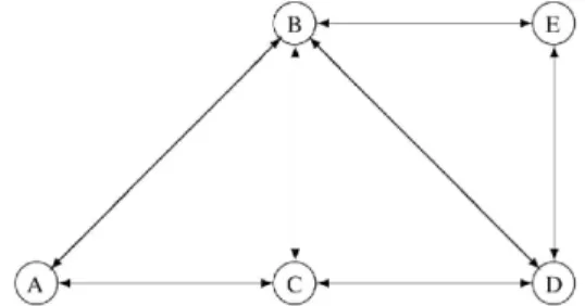
This problem is introduced in [2]. In this example, let us consider a stochastic multi-commodity network flow problem with the node set V and arc set A ⊂ V × V. For each pair of nodes (k, l)∈ V × V, there is a random quantity dkl to be shipped fromktol. The objective is to find arc capacitiesx(a), a∈ A, such that the network can carry the flows with a sufficiently large probability 1−α and the capacity expansion cost c^′x is minimized. The network structure is shown in Figure 2, and the cost factor is in Table 3. The demand is symmetric,

Figure 2: The graph of the stochastic multi-commodity network flow

From A A B B B C D

To B C C D E D E

Unit cost $310 $230 $250 $180 $350 $400 $270

Table 3: Unit costs by network arcs

i.e.,dkl=dlk for all the arcs and

dkl= 0.1D+ξkl, whereD∼N(30,5²), ξkl∼N(0, 0.25²)

The model in the original paper is a two stage stochastic programming and we need to remove the second stage variablesy(notation in [2]) and impose chance constraint on theequivalently re-written affine inequalities.

In our model, there are two types of inequalities: inequalities included in chance constraint; and inequalities as constraints formulating the feasible set.

We still usex(a), a∈ Aas the decision variable. For individual nodes, we need the incoming capacity to match the outgoing capacity. For example, node A has.

xCA+xBA=xAB+xAC (28)

where the left-hand side is the total volume of incoming capacity and the right- hand side is the total volume of outgoing capacity. The notationxAB denotes the capacity for the traffic from A to B. In addition, we need to consolidate multiple nodes as a new virtual node to avoid a potentially isolated network.

We impose the equality constraint on the virtual nodes ofA&B as the follows.

xEB+xDB+xCB+xCA =xBC+xAC+xBE+xBD (29) Similarly, the left-hand side is the total incoming capacity to the virtual node A&B, and the right-hand side is the total outgoing capacity. There is no need to impose similar equality constraint for the consolidation of three or more nodes because we only have 5 nodes in total. Constraints (28) and (29) define the feasible setX and they will not appear in the chance constraint.

Another type of inequalities will be incorporated into the chance constraint.

For individual node, we need to ensure that the random demand will be less than the capacity by large chance, i.e., 1−α. For example, nodeAimposes

xAB+xAC≥dBA+dCA+dDA+dEA (30) For the virtual node ofA&B, consolidation of nodes A and B, the inequality becomes

xBC+xAC+xBE+xBD≥dAC+dAD+dAE+dBC+dBD+dBE (31) Chance constraint includes constraint type of (30) and (31). We need to consoli- date demands as well. For example, in constraint (30), the right-hand side is the total demand from nodeA. We consolidate random variablesdBA, dCA, dDA, dEA

into one random variable. Thus, the variance-covariance matrix should be cal- culated accordingly.

From-To Exact solution SS=200 SS=500 SS=1,000 SS=10,000 SS=100,000

A-B 10.93 10.86 10.99 10.94 10.94 10.90

A-C 3.75 3.89 3.77 3.76 3.76 3.73

B-C 7.30 7.11 7.33 7.30 7.30 7.27

B-D 7.47 7.22 7.51 7.47 7.47 7.46

B-E 10.83 10.53 10.90 10.85 10.85 10.81

C-D 3.63 3.97 3.65 3.63 3.63 3.60

D-E 3.23 3.35 3.27 3.25 3.25 3.25

Time 1380s 118s 123s 140s 336s 2252s

Objective 26,981 27,274 27,149 27,031 27,031 26,859

Iterations 37 19 19 20 20 20

P(Ax≥ξ) 0.9500 0.9517 0.9490 0.9412 0.9413 0.9480

Table 4: Exact and simulation-based optimal solutions by our proposed approach, SS repre- sents the term “sample size” with starting pointx= [12; 12; 4; 4; 8; 8; 8; 8; 12; 12; 4; 4; 4; 4].

In this example, we need to show the stability of our approach under the complication of Monte Carlo. We first present the optimal solution obtained

from the exact evaluation of the joint normal distribution as the benchmark.

We then replace the exact calculation of the joint normal distribution by its sample average. We demonstrate the performances of our approach under sam- ple sizes of 200, 500, 1,000, 10,000, and 100,000 to suggest that our method will lead to stable numerical results. Surprisingly, we find that Monte Carlo leads to considerable saving in terms of calculation time; the calculation of the joint normal distribution function could be time consuming and we can only calculate the cumulative distribution function value ofξwith a limited number of dimension.

6. Concluding remarks

This paper introduced a numerical approach for the commonly encountered chance constraint optimization problem in which the chance constraint is im- posed on multiple affine inequalities with a random vector in the right-hand side. In order to preserve the convexity for both the feasible set and the chance constraint, the joint distribution of the random vector is assumed to be contin- uously log-concave. Under these assumptions, the problem is equivalent to a convex optimization problem. The primary challenge to solve such a problem is to efficiently evaluate the joint cumulative distribution function to calculate the function value and gradient. An explicit solution seems impossible because of the notoriously slow multivariate integration. We bypass the multivariate integration by adopting the sample average. We then developed a Bernstein polynomial-based approximation to obtain the functional value and the gradi- ent of the chance constraint.

Our approach controls the error of function value and the error of gradi- ent bothsimultaneously anduniformly. With the gradient mapping algorithm, the overall computational complexity will be polynomial and the optimal solu- tion, although indeed a random variable, will converge to the true optimal in probability. We implement our approach for three business analytic examples:

the financial planning, and supply chain management. The performances sug- gest that our approach yields stable solution for various scale problems. We also need to remark that the efficient implementation written in languages, especially suited to scientific computing, such as Fortran or C/C++, will considerably im- pact the overall performance. With the mainframe computational facilities, this specific type of chance constrained optimization should be solved within a timely manner.

[1] N. I. Achieser,Theory of approximation, Courier Corporation, 2013.

[2] P. Beraldi and A. Ruszczy´nski, A branch and bound method for stochastic integer problems under probabilistic constraints, Optimization Methods and Software, 17 (2002), pp. 359–382.

[3] S. Boyd and L. Vandenberghe, Convex optimization, Cambridge uni- versity press, 2009.

[4] E. Cheney, Introduction to approximation theory. 1966, Chelsea, New York.

[5] D. Dentcheva, B. Lai, and A. Ruszczy´nski,Dual methods for proba- bilistic optimization problems*, Mathematical Methods of Operations Re- search, 60 (2004), pp. 331–346.

[6] D. Dentcheva, A. Pr´ekopa, and A. Ruszczynski, Concavity and ef- ficient points of discrete distributions in probabilistic programming, Math- ematical Programming, 89 (2000), pp. 55–77.

[7] D. Jackson,The theory of approximation, New York, 19 (1930), p. 30.

[8] Y. Nesterov, Introductory lectures on convex optimization: A basic course, vol. 87, Springer, 2004.

[9] G. M. Phillips,Interpolation and approximation by polynomials, vol. 14, Springer, 2003.

[10] R. T. Rockafellar, R. J.-B. Wets, and M. Wets,Variational anal- ysis, vol. 317, Springer, 1998.

[11] A. Shapiro and P. R. Andrzej,Stochastic programming, Elsevier, 2003.

[12] A. Shapiro, D. Dentcheva, et al.,Lectures on stochastic programming:

modeling and theory, vol. 9, SIAM, 2009.

[13] G. Stewart and D. R. Kincaid, Afternotes on numerical analysis, SIAM Review, 39 (1997), p. 153.