Impulse Perturbed Stochastic Control with Application to Financial Risk Management
Dissertation
zur Erlangung des akademischen Grades Doktor der Naturwissenschaften
(Dr. rer. nat.)
Der Fakult¨ at f¨ ur Mathematik der Technischen Universit¨ at Dortmund
vorgelegt von
Laurenz M¨ onnig
Dortmund, Juni 2012
This work presents the main ideas, methods and results of the theory of impulse perturbed stochastic control as an extension of the classic stochastic control theory. Apart from the in- troduction and the motivation of the basic concept, two stochastic optimization problems are the focus of the investigations. On the one hand we consider a differential game as analogue of the expected utility maximization problem in the situation with impulse perturbation, and on the other hand we study an appropriate version of a target problem. By dynamic optimization principles we characterize the associated value functions by systems of partial differential equations (PDEs). More precisely, we deal with variational inequalities whose single inequalities comprise constrained optimization problems, where the corresponding ad- missibility sets again are given by the seeked value functions. Using the concept of viscosity solutions as weak solutions of PDEs, we avoid strong regularity assumptions on the value functions. To use this concept as sufficient verification method, we additionally have to prove the uniqueness of the solutions of the PDEs.
As a second major part of this work we apply the presented theory of impulse perturbed stochastic control in the field of financial risk management where extreme events have to be taken into account in order to control risks in a reasonable way. Such extreme scenarios are modelled by impulse controls and the financial decisions are made with respect to the worst- case scenario. In a first example we discuss portfolio problems as well as pricing problems on a capital market with crash risk. In particular, we consider the possibility of trading options and study their influence on the investor’s performance measured by the expected utility of terminal wealth. This brings up the question of crash-adjusted option prices and leads to the introduction of crash insurance. The second application concerns an insurance company which faces potentially large losses from extreme damages. We propose a dynamic model where the insurance company controls its risk process by reinsurance in form of proportional reinsurance and catastrophe reinsurance. Optimal reinsurance strategies are obtained by maximizing expected utility of the terminal surplus value and by minimizing the required capital reserves associated to the risk process.
Contents
1 Introduction 1
2 The general setup 7
2.1 Combined stochastic and impulse control . . . 7
2.2 Markov property . . . 9
2.3 Procedure . . . 10
2.4 Discussion of the model . . . 10
3 Differential game with combined stochastic and impulse control 11 3.1 Problem formulation . . . 12
3.2 Procedure and main result . . . 15
3.3 Dynamic programming . . . 18
3.3.1 From impulse control to optimal stopping . . . 19
3.3.2 DPP for optimal stopping . . . 22
3.4 Continuity of the value function . . . 25
3.5 PDE characterization of the value function . . . 26
3.5.1 Preliminaries . . . 27
3.5.2 Viscosity solution existence . . . 31
3.5.3 Viscosity solution uniqueness . . . 34
3.6 Extension of the model . . . 35
4 Stochastic target problem under impulse perturbation 43 4.1 Problem formulation . . . 44
4.2 Procedure and main result . . . 46
4.3 Dynamic programming . . . 49
4.4 PDE characterization of the value function . . . 52
4.4.1 In the interior of the domain . . . 53
4.4.2 Terminal condition . . . 54
4.5 Variant of the model . . . 55 i
5 Portfolio optimization and option pricing under the threat of a crash 57
5.1 Portfolio with 1 risky asset and n possible crashes . . . 58
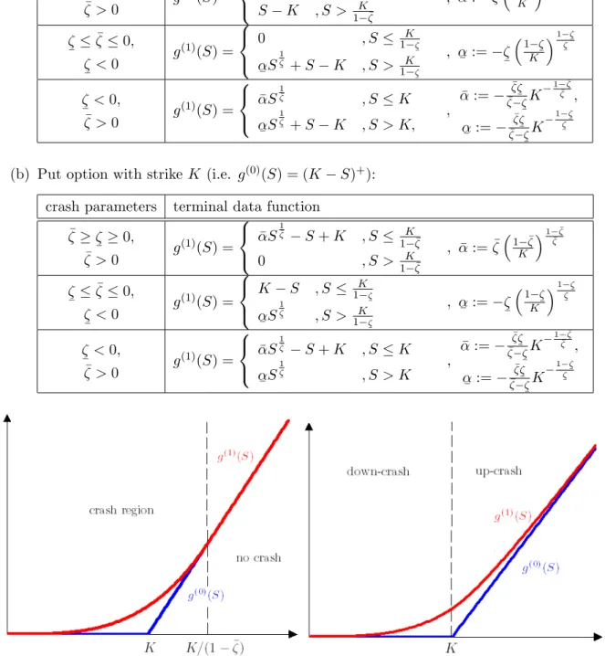
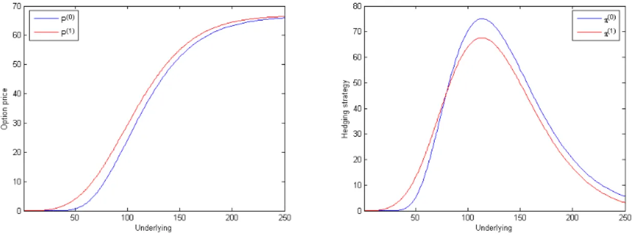
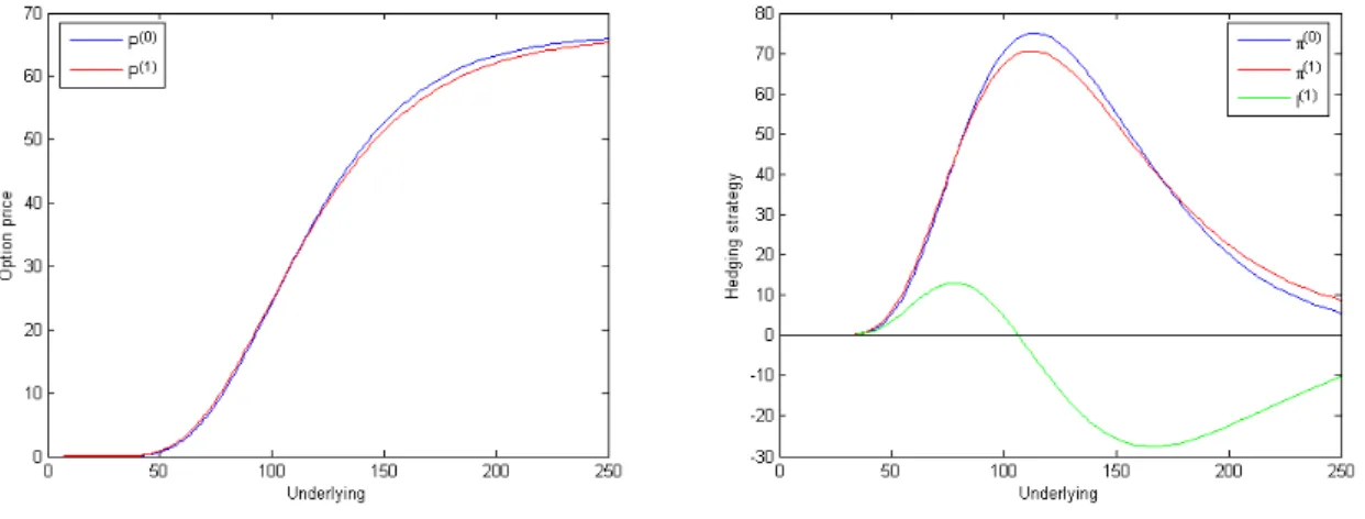
5.2 Crash-hedging via options . . . 64
5.3 Option pricing . . . 67
5.3.1 Super-hedging . . . 67
5.3.2 Market completion . . . 81
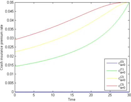
5.4 Crash insurance . . . 83
5.5 Defaultable bonds . . . 86
6 Optimal reinsurance and minimal capital requirement 91 6.1 The insurance model . . . 92
6.2 Exponential utility of terminal surplus . . . 93
6.3 Stochastic target approach . . . 99
7 Summary and conclusions 105 A Viscosity solutions of PDEs 109 A.1 Semicontinuous functions . . . 109
A.2 Definition of viscosity solutions . . . 111
A.3 Tools for uniqueness proof . . . 114
B Auxiliary tools 115 B.1 Estimates of the distribution of a jump diffusion process . . . 115
B.2 Dynkin’s formula . . . 117
B.3 Comparison theorem for ODEs . . . 118
C Proof of the PDE characterization for the target problem 121 C.1 Subsolution property on [0, T)×Rd . . . 121
C.2 Supersolution property on [0, T)×Rd . . . 123
C.3 Subsolution property on{T} ×Rd . . . 126
C.4 Supersolution property on{T} ×Rd . . . 127
Introduction
Extreme events like stock market crashes or large insurance claims can cause exceptionally large financial losses often resulting in the threat to existence for investors or insurers. To be prepared for such situations is a desirable goal. However, such rare events are difficult or actually impossible to predict in advance. In this thesis we present a type of stochastic control taking into account system crashes without modelling the crashes explicitly in a stochastic way. Under minimal assumptions concerning possible system crashes this approach aims at avoiding large losses in any possible situation.
Modelling of stock market crashes in finance or large claim sizes in insurance are actively researched mathematical topics (see, e.g., the pioneering work of Merton [37], or for a com- prehensive survey Embrechts, Kl¨uppelberg and Mikosch [14], Cont and Tankov [9] and the references therein). In the majority of cases those approaches rely on modelling the stock prices or the total claims as L´evy processes. Unfortunately, their analytical handling is not easy. Even more seriously, choosing the right distribution and fitting it to the market data is a challenging task, in particular because extreme jumps are rare events, so that there is no sufficient data available for an estimation. Another problem which arises from L´evy process models is that they neglect worst-case situations if decisions are based on expected value op- timization. So the obtained optimal solutions do not necessarily provide sufficient protection in the course of an unlike movement in the system’s state.
In contrast to modelling the extreme events in form of a stochastic jump process, we use a different control approach. The controlled state process considered in this setup is the same as if we would not take into account a possible system crash. The central idea is to amend a finite impulse control expressing system perturbation. An admissible impulse strategy represents a possible scenario with at most a fixed number of system perturbations up to the considered finite time horizon. The extent of these crashes is limited by the use of a compact set of admissible impulses. The impulse control is chosen by a virtual second agent acting as an opponent of the real decision maker, meaning that decisions are made from a worst-case point of view.
1
In summary, the main characteristics of our model are:
• Decisions are made in respect of the worst-case scenario. This guarantees best perfor- mance and the reachability of a given target relative to any possible situation.
• We focus on a finite time horizon. This parameter is of crucial importance in crash modelling because risk positions have to be adjusted to the time to maturity.
• We do not need any distribution assumption, neither for the time nor for the extent of the crash. Instead we only need the possible number of crashes within the time horizon and a range for the possible crash sizes.
Such a worst-case approach in the context of stock market crashes was firstly introduced by Hua and Wilmott [22]. They derived worst-case option prices in discrete time by replicating the option along the worst-case path by a portfolio consisting of shares of the underlying risky asset and the secure bond. In the same crash model Wilmott [58] proposed a static hedge of a portfolio against market crashes by the purchase of a fixed number of options.
Korn and Wilmott [34] took up the crash model and formulated the so-called worst-case portfolio problem in continuous time. Their work represents the first given example of impulse perturbed stochastic control. Further studies on the worst-case portfolio problem are [29], [31], [32] and [33].
The type of control dealt with in this thesis is a combination of stochastic control and im- pulse control. Nevertheless, it varies from the type of control refered to as combined stochastic control and impulse control in the literature. In [2] Bensoussan and Lions developed a general methodology for solving impulse control problems based on the concept of quasi-variational inequalities (QVIs). A QVI is a non-linear partial differential equation (PDE) consisting of a differential part combined with an impulse intervention term. Approximating impulse control by iterated optimal stopping leads to variational inequalities (VIs) in which the intervention part is given in form of an explicit constraint. If the impulse controller additionally is free to choose a control process, we are concerned with so-called Hamilton-Jacobi-Bellman (HJB) (quasi-)variational inequalities, see Øksendal and Sulem [42]. In this case one considers in the differential part the usual partial differential operator occurring in the HJB equation of stochastic control. We also refer to Seydel [52] for a deep treatment of the relation between combined stochastic and impulse control and viscosity solutions of HJBQVIs. In spite of formal similarities, our situation is not covered by the above results. This is due to the con- trary objectives of both controllers in our model. Anticipating the worst impulse strategy for any chosen stochastic control constrains the set of feasible stochastic control processes.
Therefore impulse perturbed stochastic control is related to a VI, reflecting a simultaneous optimum with respect to both the continuation (without immediate perturbation) and the perturbation situation.
Via a dynamic programming principle (DPP) we reduce impulse perturbed stochastic con- trol problems to problems of antagonistic control and stopping. By the choice of a stochastic control process the controller governs the state process, while the stopper can halt the con- trolled process at any time involving an additional cost for the controller. In particular, this cost depends on the current state of the controller’s strategy what differentiates our control problem from other already studied mixed games of control and stopping. Here most of the authors emphasize on relating mixed games to backward stochastic differential equations which are intended to characterize the value of the game (see, e.g., [12], [19]). Other ap- proaches are the reduction to a simple stopping problem [26] or a martingale approach [27].
These methods work when only the drift of the underlying state process can be controlled or under strong restrictions on the diffusion coefficients. Our approach is more direct which is possible because we work in a Markovian framework, allowing us to apply a DPP in order to link the problem to a PDE. Differential games in the context of controlled Markov processes are widely studied when both players control continuously, see for instance the monograph of Fleming and Soner [15]. To our knowledge, there are no references dealing with controller- and-stopper problems with simultaneous control of the state process and the costs due to stopping.
This work consists of two major parts, a rigorous development of the relevant theory and its applications to financial risk management. The setting of impulse perturbed stochastic control is introduced in Chapter 2. In this control framework we consider two types of problems. In Chapter 3 we analyze a differential game as analogue of the expected utility maximization problem in the situation with impulse perturbation. In this way we obtain a worst-case bound for the expected utility. In Chapter 4 we study an appropriate version of a target problem. Its objective is to determine the minimal initial value of some target process to reach a given stochastic target region at terminal time almost surely, in respect of any possible scenario. For both problems our guideline is to establish verification results under minimal assumptions. We prove that the value functions of the problems are unique viscosity solutions of a system of PDEs. Our results on the differential game are generalizations of the work of Korn and Steffensen [33] who presented a HJB-system approach (system of VIs) for solving the worst-case portfolio problem. Formulating the problem in very broad terms for controlled jump-diffusion processes and using the concept of viscosity solutions, we hope to allow for applications to a wide variety of problems. The analysis of the target problem, on the other hand, creates the theoretical foundation for the worst-case option pricing problem in [22] in a more general framework. From a mathematical point of view, we deal with a stochastic target problem for a system with jumps limited in number and size. For an introduction to stochastic target problems without jumps we refer to Soner and Touzi [54], [55]. Bouchard studied in [5] the problem when the controlled system follows a jump diffusion.
So the stochastic target problem under impulse perturbation can be regarded as the analogue of this for a finite number of jumps.
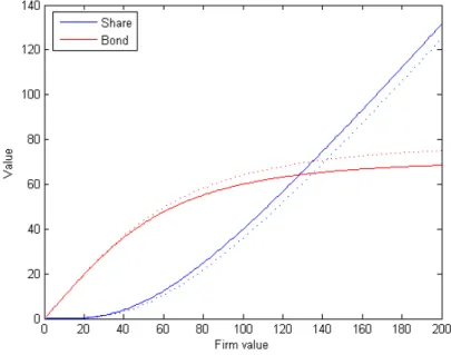
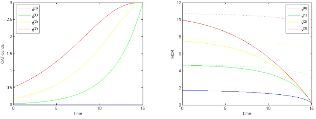
The second part of the thesis is devoted to sample applications concerning stock mar- ket crashes and large insurance claims. We solve the respective impulse perturbed control problems by using the results of the first part of the thesis, and we present some examples illustrating the shape of the value functions and the corresponding optimal strategies. In Chapter 5 we take up the worst-case portfolio problem on an extended market on which the investor can trade in stocks and derivatives to discuss crash hedging possibilities and pricing techniques for the derivatives. Besides lower and upper price bounds, which can be seen as the continuous versions of the worst-case prices derived in [22] (with a correction with respect to the terminal condition), we establish a market completion approach. To this end we consider crash insurance and calculate the insurance premium. As an application of the obtained pricing rules we introduce a valuation method for defaultable bonds. In Chapter 6 we present a new model of an insurance company utilizing impulse perturbed stochastic control to dynamically reinsure its insurance risk. Here a main focus of attention is the in- vestigation of minimal capital requirements for the insurer. Our thesis is complemented by a summary and conclusions at the end.
In sum, the most important aims of this thesis are
• the presentation of the concept of impulse perturbed stochastic control as an extension of the classic stochastic control theory,
• the generalization of the HJB-system approach presented by Korn and Steffensen [33] to differential games of stochastic control and finite impulse intervention in a very general framework with the analysis of the viscosity solution property of the value functions,
• the adaption of the stochastic target problem to impulse perturbed stochastic control,
• the application of the impulse perturbed stochastic control approach to finance (in- cluding the pricing of derivatives and crash insurance contracts in our crash model and the valuation of defaultable bonds) and insurance (computation of optimal reinsurance strategies and minimal capital requirements for a risk process under the threat of large insurance claims).
Acknowledgements
At this point, I want to thank Private Docent Flavius Guias for supervising my thesis and, in particular, for the trust he put in me. I appreciated his comments and his advice which improved my thesis considerably.
Moreover, I would like to express my thanks to Professor Ralf Korn for valuable comments and his patient explanations on stochastic control in finance. I also benefited from fruitful discussions with all the members of the Stochastic Control and Financial Mathematics Group at the University of Kaiserslautern, especially from Thomas Seifried who inspired me to new ideas on crash options and insurance.
Last, but not least, special thanks to my parents for their never-ending support.
Notation
Let us introduce some notation used throughout the thesis. Elements of Rd, d ≥ 1, are identified as column vectors, the superscriptT stands for transposition and|.|is the Euclidean norm. The i-th component of x ∈ Rd is specified by xi, and diag(x) is the diagonal matrix whose i-th diagonal element is xi. For a subset O ∈ Rd we write O for its closure, Oc for its complement and ∂O for its boundary. The open ball around x ∈Rd with radius ε > 0 is refered to as B(x, ε). If A is a quadratic matrix, then tr(A) is its trace. By Sd we denote the set of all symmetric (d×d)-matrices equipped with the spectral norm (as the induced matrix norm),Id is the identity matrix. The setC1,2 contains all functions with values inR which are once continuously differentiable with respect to the time and twice with respect to the space variables. Forϕ∈ C1,2 the notationsDxϕandD2xϕcorrespond to the gradient and the Hessian matrix, respectively, ofϕwith respect to thex variable. Forx∈Rwe also write ϕx and ϕxx. The positive and negative parts of a functionϕare denoted byϕ+= max(ϕ,0) andϕ−=−min(ϕ,0), respectively, such thatϕ=ϕ+−ϕ−.
For ease of reference, here is a partial index of notation introduced in the course of this work:
Xt,xπ,ξ, 8,12,44 Xt,xπ , 8 X(τˇ i−), 8 Et,x, 9 J(π,ξ), 12 Un, 8 Vn, 8
T, 19 Lπ, 15,46 Mπ, 15 Mπy, 46 N, 47 δN, 47,52 χU, 56
U Cx, 26 C1, 27 Pr, 38 u∗, u∗, 109
J2,+,J2,−,J¯2,+,J¯2,−, 112
The general setup
In this chapter we introduce the setting of impulse perturbed stochastic control. That is we set up the underlying state process which is controlled both continuously and by finite impulse control and which forms the basis on which we carry out our further analysis. Here the two types of control are chosen by different decision makers with contrary objectives.
After giving the controlled process along with the specific notations of finite impulse control in Section 2.1, we show in Section 2.2 the strong Markov property as fundamental property of the state process. In Section 2.3 we outline briefly the proceeding in handling stochastic control problems in this special setting, and in Section 2.4 we conclude with a short discussion on the idea of the presented model.
2.1 Combined stochastic and impulse control
LetT >0 be a fixed finite time horizon and let (Ω,F,(Ft)0≤t≤T,P) be a filtered probability space. In the classical framework of stochastic control, the state X(t) ∈ Rd of a system at timetis given by a stochastic process of the form
dX(t) =ϕ(t, X(t−), π(t−))dL(t), (2.1)
where L is a semimartingale and ϕ an appropriate function ensuring a unique solution of (2.1). The process π with values in a compact non-empty set U ⊂Rp is the control process, X = Xπ is called the (purely continuously) controlled process. We refer to the responsible decision maker concerningπ asplayer A.
Now suppose that there exists a second agent, player B, who is able to influence at any time the state of the system by giving impulses. Animpulse ζ, exercised at time twhen the system is in statexand controlled withπ, lets X jump immediately to Γ(t, x, π(t), ζ), where Γ is some given function. Notice particularly that the jump height depends on the state of control chosen from agent A. As only restriction we assume that first the allowed impulses lie in a compact non-empty set Z ⊂ Rq and second the number of allowed interventions is limited by some integern.
7
To cover situations in which player B does not intend to intervene, we assume that there exists an ineffective impulse ζ0 such that Γ(t, x, π, ζ0) = x for all (t, x, π) ∈[0, T]×Rd×U. Then we can specify the notion of an impulse control:
Definition 2.1.1. An(admissible)n-impulse control is a double sequence ξ = (τ1, τ2, . . . , τn;ζ1, ζ2, . . . ζn),
where 0 =:τ0≤τ1≤τ2≤. . .≤τn≤τn+1:=T are stopping times andζi areFτi-measurable random variables with values inZ∪{ζ0}. The stopping timeτi is calledi-th intervention time with associated impulse ζi. We denote by Vn the set of all admissible n-impulse controls.
The interventions of player B are unknown to player A a priori. But of course he notices them, so that he is able to adapt his strategy to the new circumstances. So player A will specify his action completely by a sequence of strategies π(n), π(n−1), . . . , π(0) depending on the number of intervention possibilities that are still left. At player B’s i-th intervention time player A switches immediately from the pre-intervention strategy π(n−i+1) to the post- intervention strategy π(n−i). In this context a sequence π = (π(n), . . . , π(0)) of admissible processes π(i),i= 0,1, . . . , n, describes a control for player A.
Definition 2.1.2. Denote by U0 the set of all progressively measurable processes π which have values in U and are square-integrable, i.e. E[RT
0 |π(t)|2dt]<0. Then Un:=U0n+1 is the set of all admissible (continuous) n-controls.
If we deal with a stochastic jump process, we have to distinguish at intervention timeτi
between a jump stemming from the semimartingale Land a jump caused by the impulse ζi. For this purpose we set
X(τˇ i−) :=X(τi−) + ∆X(τi),
where ∆X(τi) denotes the jump of the stochastic process without the impulse.
With the above definitions the processX =Xπ,ξ, controlled continuously byπ ∈ Un and with impulse control ξ∈ Vn, is given by
dX(t) =ϕ(t, X(t−), π(n−i)(t−))dL(t), τi< t < τi+1, i= 0, . . . , n, X(τi) = Γ(τi,X(τˇ i−), π(n−i+1)(τi), ζi), i= 1, . . . , n.
(2.2) If two or more impulses happen to be at the same time, i.e. τi+1=τi, we want to understand the jump condition in (2.2) as concatenation in form of
Γ(t,Γ(t,X(τˇ i−), π(n−i+1)(t), ζi), π(n−i)(t), ζi+1).
Let us conclude this section with some helpful notions: For (t, x)∈[0, T]×Rd, we denote by Xt,xπ,ξ the solution of the controlled SDE (2.2) with initial condition X(t) =x. In the case without impulse interventions we use the notationXt,xπ ,π∈ U0, for the solution of the purely
continuously controlled SDE (2.1). For the sake of simplicity we will omit the indicest, x, π, ξ if the context is clear. To still illustrate the dependence of the expectation on the starting point (t, x), we write
Et,x[.] :=E[.|X(t) =x].
For a given impulse control ξ ∈ Vn with intervention times τi,i= 1, . . . , n, we introduce the counting process
Nξ(t) := max{i= 0,1, . . . , n:τi ≤t}.
Then we can indicate the current control process of a controlπ∈ Un byπ(n−Nξ).
2.2 Markov property
To derive dynamic programming principles for the control problems analyzed in the following chapters, the controlled process
Yπ,ξ(t) := (t, Xπ,ξ(t), Nξ(t))
has to be a strong Markov process, i.e. for any bounded, Borel measurable function h, any stopping timeτ <∞ and allt≥0 we have
E[h(Yπ,ξ(τ +t))|Fτ] =E[h(Yπ,ξ(τ+t))|Yπ,ξ(τ)].
That means that at any arbitrary random time the processYπ,ξ“starts infresh” independently of the past. In the following we will often just say thatXπ,ξ is a strong Markov process if we refer to this affair.
It is a well known fact that the uncontrolled process ˜Y(t) := (t,X(t)), with ˜˜ X as the solution of SDE (2.1) without a control process π, has the strong Markov property, see for example Protter [46], Theorem V.32. Seydel [52] proved that the strong Markov property can be extended to controlled processes if we restrict ourselves to Markov controls. That means that the controls only depend on the current state of the system and do not use information of the past. This is the case for control processes π(i), i = 0,1. . . , n, given by some measurable feedback function ¯π(i) in form of π(i)(t) = ¯π(i)(t, X(t−)). For impulse controls the requirement of the irrelevance of the past leads to the consideration of exit times of (t,X(t−)) as intervention timesˇ τi and σ(τi,X(τˇ i−))-measurable impulsesζi.
Proposition 2.2.1(Proposition 2.3.1 in [52]). For Markov controlsπ,ξthe controlled process Yπ,ξ(t) is a strong Markov process.
As a consequence of this proposition, from now on we consider exclusively Markov controls, i.e. we suppose that the admissibility setsUn,Vn only contain such controls.
2.3 Procedure
In this thesis we analyze two types of control problems. In Chapter 3 we study a differential game where player A tries to maximize some objective functionJ, whereas player B intends to minimize J. In Chapter 4 we deal with a target problem in the form that we want to determine the minimal initial valueY(0) =yof some target processY that allows player A to reach a given target Y(T)≥g(X(T)) at final time almost surely, whatever player B attemps to prevent him from that. In both cases the solution is obtained by an iterative proceeding:
Step 0. We start with computing the solution of the control problem without impulse control.
Step n. Given the solution of the (n−1)-impulse control problem we can reduce the n-intervention problem to an impulse problem with only one intervention possibility.
2.4 Discussion of the model
The generated strategies secure best performance and the reachability of a given target, re- spectively, relative to any possible situation, in particular they arecrash-resistant. Moreover, the basic assumptions of the model are very simple. We do not need any distribution assump- tions for jumps due to impulses, neither for the jump time nor for its height. Of course the assumption of a limited finite number of possible perturbations is critical. This restriction is not urgently necessary. But for an unbounded intervention number there exists the risk of no end of interventions in an instant. To avoid these constellations we would have to weaken the effects of an impulse in a way that guarantees non-optimality of such degenerate intervention strategies. But this is inconsistent to the intention of modelling extreme situations where we want to understand the impulse interventions as rare events with grave consequences. So a small number of interventions reflects exactly the characteristic feature of such catastrophes.
Of course there are several extensions of the model which are possible. For example we could allow for time- and state-depending sets U(t, x) and Z(t, x). Else the assumption of a compact control set U could be dropped. Both changes would lead to other additional requirements on the admissible setU0which provide for existence and uniqueness of a solution of the state equation (2.2). Moreover, we could include a possible regime switch as result of an intervention by using different coefficients ϕ(n−i), i= 0,1, . . . , n, in (2.2). For example, think of a capital market where a crash usually leads to an increase in volatility, see Korn and Menkens [31] for results of crash hedging with changing market parameters. However, to keep the notation as easy to get along with, we neglect these generalizations.
Differential game with combined stochastic and impulse control
In this chapter we investigate a stochastic worst-case optimization problem consisting of stochastic control and impulse control. This problem corresponds to the maximization of the expected utility of a state process in consideration of system crashes, where crash scenarios are modelled by impulse interventions and we maximize with respect to the worst-case scenario.
The motivation of this problem comes from the portfolio problem under the threat of market crashes. Hua and Wilmott introduced in [22] a crash model where the sudden drops in market prices are not modelled stochastically. Based on very simple assumptions on possible crashes, they chose a worst-case approach to manage the crash risk in any possible situation.
While [22] is focused on the pricing of options in discrete time, Korn and Wilmott [34] applied this approach in the context of continuous-time portfolio optimization. They formulated the portfolio problem as a differential game in which the investor meets the market as an opponent who systematically acts against the interests of the investor by causing crash scenarios. In this way they obtained portfolio strategies that maximize the worst-case bound of the investor’s utility. In this chapter we basically refer to Korn and Steffensen [33] who presented a HJB- system approach (system of inequalities) for solving the worst-case portfolio problem. Our results are generalizations of their work, in particular we do not require strong regularity assumptions on the value function by using the concept of viscosity solutions. Examples for further studies of the worst-case portfolio problem with respect to market crashes are [29], [31] and [32]. Moreover, there are similar worst-case approaches in the context of portfolio optimization for considering model risk (see, e.g., [20], [38] and [56] and the references therein).
A reference for deterministic worst-case design with numerous examples and applications to risk management is the book of Rustem and Howe [47].
To start with we present in Section 3.1 a detailed problem formulation including all assumptions we make. In the next section we state a PDE characterization of the associated value function in the viscosity sense as main result of this chapter, and we explain in more
11
detail how we want to proceed in the following to prove this viscosity property. The main steps are the transformation of the problem and the derivation of a dynamic programming principle in Section 3.3, the proof of the continuity of the value function in Section 3.4 and its characterization as a unique viscosity solution in Section 3.5. An extension of the model and a relaxation of assumptions is discussed in the last section.
3.1 Problem formulation
Let T >0 denote a fixed finite time horizon and let (Ω,F,(Ft)0≤t≤T,P) be a filtered prob- ability space satisfying the usual conditions, i.e. the filtration (Ft)t is complete and right- continuous. We consider further an adapted m-dimensional Brownian motion B and an adapted independent k-dimensional pure-jump L´evy processL. We denote by
N˜(dt, dz) =N(dt, dz)−ν(dz)dt
its compensated Poisson random measure with jump measureNand L´evy measureν. Through- out this chapter we assume that
Z
|z|≥1
|z|ν(dz)<∞. (3.1) This condition gives us the L´evy-Itˆo-decomposition in form of
L(t) = Z t
0
Z
z∈Rk
zN˜(ds, dz).
For more precise definitions and properties of random measures we refer to Jacod and Shiryaev [24] or Sato [49]. On this stochastic basis we consider the process X = Xπ,ξ, controlled continuously by π ∈ Un and with impulse controlξ ∈ Vn, given by
dX(t) =µ(t, X(t), π(n−i)(t))dt+σ(t, X(t), π(n−i)(t))dB(t) +
Z
Rk
γ(t, X(t−), π(n−i)(t−), z)dN˜(dt, dz), τi < t < τi+1, i= 0, . . . , n, X(τi) = Γ(τi,X(τˇ i−), π(n−i+1)(τi), ζi), i= 1, . . . , n.
(3.2)
Here the functions µ: [0, T]×Rd×U →Rd, σ : [0, T]×Rd×U →Rd×m,γ : [0, T]×Rd× U ×Rk → Rd and Γ : [0, T]×Rd×U ×Z → Rd satisfy conditions detailed in Assumption 3.1.1 below.
As performance criterion we consider a functional of the form J(π,ξ)(t, x) =Et,x
Z T t
f(s, X(s), π(n−Nξ(s))(s))ds+g(X(T))
+ X
t≤τi≤T
K(τi,X(τˇ i−), π(n−i+1)(τi), ζi)
,
wheref : [0, T]×Rd×U →R,g :Rd →R and K : [0, T]×Rd×U ×Z →R are functions satisfying conditions detailed in Assumption 3.1.1 below. Heref can be interpreted as running profit, g as end profit and K stands for the additional profit resulting from an impulse intervention (or, from another point of view, as loss, respectively). Bearing in mind the role ofζ0 as ineffective impulse, we assumeK(t, x, π, ζ0) = 0 for all (t, x, π)∈[0, T]×Rd×U.
In view of player B’s role as creator of system perturbation we suppose that both players have contrary objectives. While player A tries to maximize J, player B is intended to minimizeJ. In order to reach their aims both players select their respective strategy from their admissibity setsUnandVn, respectively. First agent A settles his control π. Depending on this choice his opponent B decides to intervene or not. So our stochastic optimization problem reads as follows: Findoptimal controls ˆπ ∈ Un, ˆξ∈ Vnwith associatedvalue function v(n) such that
v(n)(t, x) = sup
π∈Un
ξ∈Vinfn
J(π,ξ)(t, x) =J(ˆπ,ξ)ˆ(t, x). (3.3) Such two-player-games with contrary objectives are called differential games. So the prob- lem (3.3) represents a stochastic differential game combining stochastic control and impulse control.
Now let us summarize the conditions that form the basis for the investigation of the value functionv(n) in the following assumption:
Assumption 3.1.1. (G1) The control set U ⊂Rp and the impulse setZ ⊂Rq are compact and non-empty.
(G2) The functionsµ, σ,γ are continuous with respect to (t, x, π), γ(t, x, π, .) is bounded for
|z| ≤1, and there exist C >0, δ :Rk →R+ withR
Rkδ2(z)ν(dz) <∞ such that for all t∈[0, T], x, y∈Rd and π∈U,
|µ(t, x, π)−µ(t, y, π)|+|σ(t, x, π)−σ(t, y, π)| ≤C|x−y|,
|γ(t, x, π, z)−γ(t, y, π, z)| ≤δ(z)|x−y|,
|γ(t, x, π, z)| ≤δ(z)(1 +|x|).
(G3) The transaction functionΓand the profit functionsf,g,K are continuous and Lipschitz in x(uniformly int,π andζ), i.e. there is a constantC >0such that for allt∈[0, T], x, y∈Rd, π∈U and ζ ∈Z,
|Γ(t, x, π, ζ)−Γ(t, y, π, ζ)|+|f(t, x, π)−f(t, y, π)|
+|g(x)−g(y)|+|K(t, x, π, ζ)−K(t, y, π, ζ)| ≤C|x−y|.
The assumptions (G1) and (G2) guarantee the existence of a unique strong solution to (3.2) with initial condition X(t) =x ∈Rd (for general existence and uniqueness results for SDEs with random coefficients see Gichman and Skorochod [17] or Protter [46]). The assump- tion (G3) implies that Γ, f,g,K satisfy a global linear growth condition with respect to x.
Therefore the objective function J is well-defined and, using the estimate (B.2) of Lemma B.1.1 together with the tower property of conditional expectation (see the argumentation in the appendix subsequent to Lemma B.1.1), we can conclude that
|v(n)(t, x)| ≤C(1 +|x|) (3.4)
for some constantC >0 independent oft, x.
Example 3.1.1. Consider the controlled deterministic process dX(t) =−απ(1)(t)dt, t∈(0, τ1), X(τ1) =X(τ1−)−(1−π(1)(τ))ζ1, dX(t) =−απ(0)(t)dt, t∈(τ1, T),
with parameterα >0, 1-impulse perturbation (τ1, ζ1)∈[0, T]×({ζ}∪{0}),ζ >0, and control π = (π(1), π(0)) whose processes have values in [0,1], i.e. the setting is n = 1, U = [0,1], Z ={ζ}.
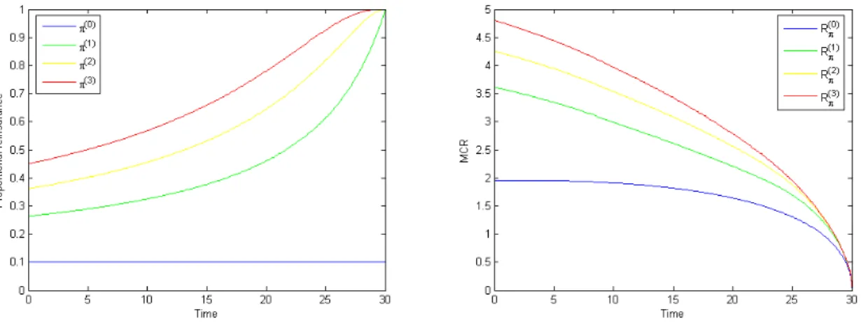
For an interpretation think of an insurer who is faced with one possible claim of sizeζ up to time T. To limit the risk exposure the insurer can reinsure a proportionπ of the claim by paying a continuous reinsurance premium α. If the claim is admitted at timeτ, the insurer has to pay the sum (1−π(τ))ζ. The controlled processX then reflects the insurer’s surplus.
We now want to maximize the expected value of X(T) in the worst-case sense, i.e. we consider the differential game
v(1)(t, x) = sup
π∈U1 ξ∈Vinf1
Eπ,ξt,x[X(T)],
where U1,V1 are the sets of admissible controls introduced in the preceding chapter.
It is easy to check that (G1)-(G3) from Assumption 3.1.1 are satisfied for this problem formulation. So the controlled process as well as the differential game are well-defined.
Step 0. If there is no perturbation to fear, it cannot be optimal to pay for protection against one. So we have v(0)(t, x) =x with ˆπ(0) ≡0.
Step1. By intuition we try to determine the optimal strategy ˆπ(1) and the value function v(1) via an indifference consideration. We demand as much protection as to be left with the same final expected value, regardless of the occurrence of a perturbation. So choose ˆπ(1) such that
x−(1−πˆ(1)(t))ζ =x− Z T
t
αˆπ(1)(s)ds. (3.5)
The left hand side of (3.5) is the expected value for an immediate impulse intervention and the right hand side is the expected value without impulse intervention. To be indifferent at final time we require ˆπ(1)(T) = 1. Subtracting x in (3.5), it seems that the optimal control process ˆπ(1) is independent of the state ofX, so that the process coincides with its feedback function. Differentiating on both sides of (3.5) we obtain a ODE for ˆπ(1),
∂
∂tπˆ(1)(t) = α
ζˆπ(1)(t), πˆ(1)(T) = 1.
Solving this ODE and calculating the corresponding value of one side of equation (3.5), we conclude
v(1)(t, x) =x−
1−exp
−α
ζ(T −t)
ζ, π(1)(t) = exp
−α
ζ(T−t)
.
We will verify in the next subsection that this is indeed the solution to our problem. Just note that the strategy ˆπis admissible since ˆπ(i),i= 1,2, has values inU, is Markovian (given in form of some feedback function) and progressively measurable (because it is deterministic).
3.2 Procedure and main result
In the rest of this chapter we devote ourselves to the characterization of the value function v(n) as the unique viscosity solution of a system of PDEs. To formulate the corresponding PDEs we introduce for a valueπ ∈ U the Dynkin second order integro-differential operator Lπ associated to the processXπ (with constant controlπ(.)≡π),
Lπϕ(t, x) = ∂ϕ
∂t(t, x) +µ(t, x, π)TDxϕ(t, x) +1
2tr (σσT)(t, x, π)Dx2ϕ(t, x) +
Z
Rk
{ϕ(t, x+γ(t, x, π, z))−ϕ(t, x)−γ(t, x, π, z)TDxϕ(t, x)}ν(dz),
(3.6)
and theintervention operator Mπ transacting the best immediate impulse for player B, Mπϕ(t, x) = inf
ζ∈Z{ϕ(t,Γ(t, x, π, ζ)) +K(t, x, π, ζ)}. (3.7) Supposed n interventions might happen, it seems reasonable for player A to choose at the point (t, x) a control policy π ∈ U0 fulfilling v(n)(t, x) ≤ Mπ(t)v(n−1)(t, x). Otherwise an immediate intervention would dissuade player A from achieving the optimal utilityv(n)(t, x).
To be able to preserve a similar optimality condition for approximately optimal controls also after starting timet, we need the following additional requirement:
Assumption 3.2.1. For all (t, x) ∈[0, T)×Rd and ε >0 there exists an ε-optimal control π∈ Un in the sense of
ξ∈Vinfn
J(π,ξ)(t, x)≥v(n)(t, x)−ε,
whose feedback functionsπ¯(i), i.e. π(i)(t) = ¯π(i)(t, X(t−)), are continuous.
In particular, this assumption is satisfied if the optimal control itself has continuous feedback functions. For one part of the characterization of the value function (see the sub- solution property in Theorem 3.5.5 below) we will use the following consequence: For π as in Assumption 3.2.1 we can find for any δ > ε a neighborhood B of (t, x) such that Mπ(s)v(n−1)(s, y)≥v(n)(s, y)−δ for all (s, y)∈ B.
In the following we show how the differential game with at mostnintervention possibilities can be solved iteratively:
Step 0. We start with computing the value function v(0) of the classic pure continuous control problem. This problem is studied extensively in the existing literature, also for jump processes (see, e.g., Øksendal and Sulem [42]), so that we already know thatv(0) is a viscosity solution of the Hamilton-Jacobi-Bellman equation (HJB-equation)
π∈Uinf{−Lπv(0)−f(., ., π)}= 0 on [0, T)×Rd, v(0)−g= 0 on {T} ×Rd.
(3.8) Step n. Given the value function of the (n−1)-differential game we can transfer the n-intervention problem into a one time stopping problem with a final payoff depending on v(n−1). Then it turns out that the value function v(n) is a viscosity solution of the equation
π∈Uinf max
−Lπv(n)−f(., ., π), v(n)− Mπv(n−1)
= 0 on [0, T)×Rd, v(n)−min
g,sup
π∈U
Mπv(n−1)
= 0 on {T} ×Rd.
(3.9)
Note that (3.8) and (3.9) are partial integro-differential equations. The precise definition of a viscosity solution in this case (with a non-local integral term) is given in Section 3.5.
Further we will prove the uniqueness of a viscosity solution of (3.8) and (3.9) in a special class of functions, so that we can be sure that a solution of the respective equation is indeed the seeked value function.
Compared to existing results on combined stochastic and impulse control, the special quality of the equation (3.9) is the simultaneous minimization with respect to the control π of both the differential and the impulse part. This illustrates the balance problem of player A who has to find a strategy that is optimal with respect to the worse case of no intervention at the moment (first argument in the max-term) and an immediate impulse of the most horrendous proportion (second argument in the max-term). If the effects of player B’s impulses did not depend on player A’s strategy, the impulse component in (3.9) would not depend on π any more, so that we could move the infimum within the first argument of the max-term resulting in the so-called Hamilton-Jacobi-Bellman variational inequality (HJBVI). That means that player A would not be restricted any more in his decision and could concentrate on his performance in intervention-free times. On the other hand player A is at player B’s mercy because A cannot influence the consequences resulting from impulses at the intervention times. But in view of applications to risk management we are of course especially interested in limiting the loss even in the extreme situations.
Following Korn and Steffensen in [33] we could also state the value function on [0, T)×Rd as solution of a variational inequality of two constrained optimization problems:
max
π∈Uinf2
{−Lπv(n)−f(., ., π)}, inf
π∈U1
{v(n)− Mπv(n−1)}
= 0,
where we minimize on the subsets
U1 ={π∈U :−Lπv(n)−f(., ., π)≤0}, U2 ={π∈U :v(n)− Mπv(n−1) ≤0}.
Note that Ui = Ui(t, x, n), i = 1,2, are not given explicitly because they depend on the studied value function.
Before going any further, we want to validate the above equations for the derived solution of the deterministic Example 3.1.1.
Example3.2.1 (Continuation of Example 3.1.1). We concentrate on the PDE characterization forv(1) and recall our guess from Example 3.1.1,
v(1)(t, x) =x−
1−exp
−α
ζ(T−t)
ζ.
In view of the dynamics of the controlled process given in Example 3.1.1 we calculate Lπv(1)(t, x) = ∂
∂tv(1)(t, x)−απ ∂
∂xv(1)(t, x) =α
exp
−α
ζ(T −t)
−π
, and from the jump condition related to an impulse we get
v(1)(t, x)− Mπv(0)(t, x) =x−
1−exp
−α
ζ(T−t)
ζ−(x−(1−π)ζ)
=ζ
exp
−α
ζ(T −t)
−π
. So the PDE in (3.9) reads
π∈[0,1]inf max
α
π−exp
−α
ζ(T−t)
, ζ
exp
−α
ζ(T −t)
−π
= 0. (3.10) We see that the max-term in (3.10) is zero for
π=π(1)(t) = exp
−α
ζ(T−t)
∈[0,1]
and strictly positive else. So we have found a minimizer for the left hand side of (3.10) with minimum zero. So v(1) fulfills equation (3.10). Furthermore, the terminal condition is satisfied because of
v(1)(T, x) =x= min x, sup
π∈[0,1]
{x−(1−π)ζ}
! ,
where the above supremum is realized byπ =π(1)(T) = 1. This ends our validation which confirms the predications of Example 3.1.1.
The rest of this chapter is organized as follows: From now on we assumen≥1. Then we start in Section 3.3 with the derivation of a dynamic programming principle (DPP) which is associated to the stochastic differential game. More precisely, we will state two versions of a DPP. The first one establishes the connection ofv(n)to the value functionv(n−1)of the inferior problem. Here we point out that the impulse part of the control problem can be reduced to a problem of finding an optimal stopping time for the first intervention. The solution of the differential game with n intervention possibilities thus turns out to be an iteration of n differential games combining stochastic control and optimal stopping. Afterwards we give a second version of a DPP which is similar to the classic principles in which the controlled system is analyzed up to some stopping timeτ while it is supposed to be controlled optimally in the sequel. The value function v(n) at initial state (t, x) is then refered to itself at the stochastic state (τ, X(τ)). After showing in Section 3.4 that v(n) is continuous, we use this representation of v(n) in Section 3.5 to point out the connection to the PDE (3.9). Since we cannot guarantee that v(n) is smooth enough, we use the concept of viscosity solutions as weak solutions of PDEs. This gives us a necessary condition for the value function in contrast to a traditional verification theorem (applicable only under strong regularity requirements) which presents a sufficient condition. However, the concept of viscosity solutions only makes sense if we can be sure that a viscosity solution is indeed the seeked value function. So we have to deal with the question of uniqueness of viscosity solutions of PDE (3.9) in the sequel. We conclude this chapter in Section 3.6 with a discussion on an extension of the model framework including relaxed assumptions.
In this chapter we follow Korn and Steffensen [33] where a special differential game of our type is analyzed, in particular for the derivation of the first DPP. For the handling of a differential game combining stochastic control and optimal stopping, we copy techniques of Pham [44] who studied optimal stopping of controlled jump diffusion processes.
3.3 Dynamic programming
In this section we provide a DPP for our differential game that we want to use in the following to characterize the value function as viscosity solution of a PDE.
We proceed in two steps: First we transform the original problem with impulse control into a problem associated with combined stochastic control and optimal stopping. Then we derive a DPP for optimal stopping of a controlled process.
Before doing so, we need to discuss some essential requirements. The basic idea of dy- namic programming is to split the problem into subproblems, so that the optimal solution is composed of the solutions of the separate parts. For this method to work, two properties of the controlled process and the admissible controls are crucial. Firstly, the admissibility sets have to be stable under concatenation. This means that for any stopping timeτ ∈[0, T] a control switching at time τ from one admissible control to another admissible one is ad-
missible, too. This condition guarantees the admissibility of the composition of solutions of subproblems. Secondly, splitting the relevant time interval [t, T] into [t, τ) and [τ, T] and observing the system on the latter one separately, it is necessary that, given the state at time τ, the system is independent of its course on [t, τ). This requirement corresponds to the strong Markov property of the underlying process which actually is satisfied in our case according to Proposition 2.2.1.
3.3.1 From impulse control to optimal stopping
For a first version of a DPP we consider the problem up to the first intervention and the problem withn−1 remaining intervention possibilities as isolated cases. For this decomposi- tion of the problem the stability assumption onUn,Vnis obviously satisfied in the following sense:
• If π(n) ∈ U0 and π0= (π(n−1), . . . , π(0))∈ Un−1, thenπ = (π(n), π(n−1), . . . , π(0))∈ Un.
• If (τ1;ζ1) ∈ V1 and ξ0 = (τ2, . . . , τn;ζ2, . . . , ζn) ∈ Vn−1 such that τ1 ≤ τ2, then ξ = (τ1, τ2, . . . , τn;ζ1, ζ2, . . . , ζn)∈ Vn.
Recall that Xπ = Xt,xπ denotes the controlled process with start in (t, x) ∈ [0, T]×Rd under control π ∈ U0 and no impulse intervention. We define by T = T(t) the set of all stopping timesτ ∈[t, T] which represent admissible intervention times in the sense that they are independent of the past. Further we recall the definition of the intervention operatorMπ from (3.7).
Now we can state the first important result of this section which is a generalization of Lemma 2 in Korn and Steffensen [33]. For the problem of optimization of the final utilility of a diffusion process with impulse perturbation (with fixed impulseζ) they derived the relation
v(n)(t, x) = sup
π∈U0
τ∈Tinf Et,x
h
v(n−1)(τ,Γ(τ, Xπ(τ−), π(τ), ζ)) i
.
We notice that this result implies that intervening is the optimal strategy for player B which is not true in general. Moreover, in view of our general choice of the performance criterion, we need to take into consideration the utility functions f, g and K as well as different admissible impulses. However, the correct version in our case is very intuitive and can be derived similarly to the lemma in [33].
Theorem 3.3.1 (Dynamic programming principle (version 1)). The value function v(n) in (3.3)can be represented in form of
v(n)(t, x) = sup
π∈U0
τ∈Tinf Et,x
Z τ t
f(s, Xπ(s), π(s))ds
+Mπ(τ)v(n−1)(τ, Xπ(τ))1{τ <T}
+ min
g,Mπ(τ)v(n−1)
(τ, Xπ(τ))1{τ=T}
.
(3.11)
Proof: Fix (t, x) ∈ [0, T]×Rd and consider an impulse control ξ ∈ Vn which is com- posed of the first intervention (τ1;ζ1) and ξ0 := (τ2, . . . , τn;ζ2, . . . , ζn). On the stochastic interval [t, τ1) the continuous control given by π = (π(n), . . . , π(0)) ∈ Un equals π(n). Af- terwards it switches to the (n−1)-control π0 := (π(n−1), . . . , π(0)). For each path with no intervention in the relevant time interval [t, T], we are free to set τ1 = T and ζ1 = ζ0. Noting that ˇXπ,ξ(τ1−) = Xπ(n)(τ1) the controlled process jumps at intervention time to x0:= Γ(τ1, Xπ(n)(τ1), π(n)(τ1), ζ1). Since E[.|Ft] =E[E[.|Fτ1]|Ft] holds for allτ1 ≥tand any controlled process has the strong Markov property, we can state the objective functional in form of
J(π,ξ)(t, x) =Et,x
Z τ1
t
f(s, Xπ(n)(s), π(n)(s))ds+K(τ1, Xπ(n)(τ1), π(n)(τ1), ζ1)
+Eτ1,x0
Z T τ1
f(s, Xπ0,ξ0(s), π(n−1−Nξ
0(s))(s))ds+g(Xπ0,ξ0(T))
+ X
τ1≤τi≤T i≥2
K(τi,Xˇπ0,ξ0(τi−), π(n−i+1)(τi), ζi)
. To make the notation more convenient we set
Yπ(n),(τ1;ζ1):=
Z τ1
t
f(s, Xπ(n)(s), π(s))ds+K(τ1, Xπ(n)(τ1), π(n)(τ1), ζ1).
Then, using the definition of the objective functionalJ we obtain J(π,ξ)(t, x) =Et,x
h
Yπ(n),(τ1;ζ1)+J(π0,ξ0)(τ1, x0)i
. (3.12)
Letε >0. For a given first intervention (τ1;ζ1) choose a control ˆπ∈ Unthat is ε2-optimal both up to the first intervention and later on, i.e.
sup
π(n)∈U0
Et,x
h
Yπ(n),(τ1;ζ1)+v(n−1)(τ1, x0)i
≤Et,x
h
Yˆπ(n),(τ1;ζ1)+v(n−1)(τ1,xˆ0)i + ε
2, (3.13) sup
π0∈Un−1
ξ0∈Vinfn−1
J(π0,ξ0)(τ1,xˆ0)≤ inf
ξ0∈Vn−1
J(ˆπ0,ξ0)(τ1,xˆ0) + ε
2, (3.14)
where ˆx0 = Γ(τ1, Xπˆ(n)(τ1),πˆ(n)(τ1), ζ1) is the state after the first intervention (τ1;ζ1) if the strategy ˆπ(n) is applied until the first intervention. Furthermore, for a given control π ∈ Un choose an impulse intervention ˆξ ∈ Vn that is ε2-optimal both for the first intervention and in the sequel, i.e.
τinf1∈T ζ1∈Z∪{ζ0}
Et,x
h
Yπ(n),(τ1;ζ1)+v(n−1)(τ1, x0) i
≥Et,x
h
Yπ(n),(ˆτ1; ˆζ1)+v(n−1)(ˆτ1,xˆ0) i
− ε
2, (3.15)
ξ0∈Vinfn−1
J(π0,ξ0)(τ1,xˆ0)≥ J(π0,ξˆ0)(τ1,xˆ0)−ε
2, (3.16)