ABSTRACT
The DASH model for Power Portfolio Optimization provides a tool which helps decision-makers coordinate production decisions with opportunities in the wholesale power market. The methodology is based on a stochastic programming model which selects portfolio positions that perform well on a variety of scenarios generated through statistical modeling and optimization. When compared with a commonly used fixed-mix policy, our experiments demonstrate that the DASH model provides significant advantages over several fixed-mix policies.
1 INTRODUCTION
Deregulation is an evolving process. In many states (including Arizona), the major electricity producers have the responsibility of meeting a certain “native load” which constitutes the regulated portion of the business. Beyond this regulated native load, a power producer may buy or sell power in the wholesale electricity market in a manner that the producer finds profitable. Prior to the emergence of electricity markets, profitability was determined simply by the ability of a power producer to convert fuel into electricity in a least-cost manner. Hence minimization of generation costs provided the appropriate strategy. With the emergence of wholesale electricity markets, a utility can manage its power production and revenue potential by trading within this market. A forward (contract) for power is a financial instrument that allows a power producer to buy or sell power for delivery on a future (maturity) date at a price that is agreed upon several months earlier. As weather patterns, economic activity, and market prices evolve, these power portfolios can be rebalanced so as to maximize expected profitability, while A STOCHASTIC PROGRAMMING APPROACH TO POWER PORTFOLIO OPTIMIZATION
Suvrajeet Sen Lihua Yu Talat Genc
Raptor Laboratory, SIE Department, University of Arizona,
Tucson, AZ 85721,U.S.A.
December 3, 2002
appropriately balancing risk exposure. In this environment, judicious decision-making can mean the difference between survival and demise of a power company.
The DASH model for Power Portfolio Optimization provides a tool which helps decision-makers coordinate production decisions with opportunities in the wholesale power market. Before providing the technical details of our approach, we provide a brief outline of some of the major determinants of profitability in electricity markets. Following this description, we describe statistical models that are used for developing scenarios used within the stochastic programming model. The latter model consists of a financial sub-model and a generation sub-model which are used to determine the profitability of any portfolio position. We also describe an alternative investment strategy based on a certain type of “fixed- mix” policy which is commonly used by electricity traders. This strategy provides a “base-case” against which we compare the results of a stochastic programming model. Our results are based on data obtained from Pinnacle West Capital, which is a holding company for Arizona Public Service, the largest investor owned electric utility in Arizona. In order to maintain confidentiality of their data, our results will be presented in terms of percentage gain. The backcasting experiment, which covers a five month operating period from January 2001 through May 2001, shows a monthly advantage of approximately 7% in favor of the stochastic programming approach. The DASH model has also been tested against a variety of synthetic scenarios. These experiments reveal the robustness of the forward decisions recommended by DASH.
1.1 Contributions of this paper
Portfolio optimization models have been investigated using stochastic programming in many recent papers (e.g. Carino and Ziemba (1998), Wu and Sen (2000)), and the volume edited by Ziemba and Mulvey (1998) provides extensive coverage of asset/liability modeling. By the same token the electric utility industry has also applied stochastic programming for hydro-electric generation scheduling (Jacobs et al. (1995)), unit commitment under uncertainty (e.g. Takriti, Kasenbrink, Wu, (2000), Nowak and Romisch (2000)). Fleten, Wallace and Ziemba (2002) have discussed a model that combines hydro- electric systems scheduling as well as investments in electricity markets. Our paper is in the spirit of their work, although our modeling approach is significantly different. We provide a comprehensive approach in which statistical models of the markets and decision models of the producer are integrated, and the methodology is evaluated through extensive simulation experiments. We propose spot market and power generation models that operate on a fine enough time-scale to allow for modeling on-peak as
well as off-peak electricity products and electricity generation. In addition we allow a variety generators within a fine grain unit commitment model. On the financial side we allow contracts to be modeled on a larger time scale (i.e. monthly) and moreover include both electricity and gas markets. Since gas is often the marginal fuel used by power producers facing peak-load, modeling the gas market provides much more realistic estimates of future marginal cost of electricity. Our model captures the impact of generation costs (which are typically obtained from short term unit-commitment models) on investments in electricity commodities (typically on a monthly time-scale). This multi-granularity approach allows much greater fidelity than has been attempted to date. Naturally, the resulting model is far too complex for solution using off-the-shelf MILP solvers.
We design a new nested column generation approach that decomposes the model into smaller subproblems which are coordinated within the new algorithm. In addition to providing an algorithmically tractable approach, this new algorithm maintains modularity by solving a fine grain (electricity generation) model and a coarse grain (financial investment) model separately. Another important advantage of the new algorithm is that it is relatively straightforward to study a sequence of instances, with alternative probability estimates for the scenarios. This is because the method is based on column generation, and changes in probability distribution only shows up in the objective function of the model. Thus, the new algorithm is amenable for day-to-day implementations in which probability estimates may evolve, and new instances may have to be resolved.
Finally, this paper also describes our statistical modeling effort for scenario generation in the decision phase, as well as the evaluation phase. The scenarios generated for the decision phase are used within the stochastic programming model, whereas, scenarios used in the evaluation phase are meant to test the robustness of decisions provided by the stochastic programming (DASH) model. Thus, our paper provides a comprehensive treatment including statistical modeling, optimization, and simulation.
2 SCOPE OF THE DASH MODEL
To begin with, we outline the manner in which we expect the decision process to unfold. At the start of each month, financial analysts/traders for the producer wish to reevaluate/rebalance their power portfolio. At this point, they may invoke some decision model (e.g. DASH) which recommends the mix of power products that the producer ought to hold. While the decision model itself may be dynamic (as
in DASH), the trader only commits to a recommendation for the current month. After the appropriate rebalancing trades are executed, the traders wait and observe the market until the end of the month, at which point, they update the decision model by “rolling the horizon” forward, and providing up-to-date information to the decision model which then provides an updated recommendation for the next month.
While it is possible to use the DASH model at decision-epochs that are less than a month long, the portfolios within DASH are represented at monthly intervals.
Market modeling is another feature incorporated within DASH. In some cases, power producers trade electricity in multiple markets. For example, a California utility may trade in Palo Verde (AZ) and the California-Oregon Border (COB). For the sake of this model however, we will consider only one market for electricity. In addition to electricity, the model also allows interactions with one natural gas market. On the generation-side, the unit commitment decisions are made on a monthly basis, and allow us to incorporate heat-rates, start-up costs, minimum downtimes, etc. The current model does not accommodate hydro generation, although this extension is currently under consideration.
2.1 Electricity Demand
In a completely deregulated market, the traditional notion of load takes a back-seat to demand-curves relating prices and quantities. However the extent of deregulation is in a state of flux in most states in the U.S. For instance in Arizona, retail tariffs are regulated by the state Corporation Commission and are held constant over long periods of time. Electric utilities are required to serve the “native load” that arises from their customers at regulated retail rates. There are several different demand models that have been studied in conjunction with current the DASH model, including time-series that use temperature as one of the main factors. In more humid climates, we expect that humidity will play an important role as well (Feinberg (2002)).
2.2 The Wholesale Electricity Market
The current market model allows electricity forward contracts, and spot market activity. While the current model does not accommodate options, these can be included without adding to the computational burden of the current model. While prices in the electricity market (especially the spot market) vary on an hourly basis, we have discretized time according to a sixteen hour “on-peak” period, and an eight hour “off-peak” period for each day.
2.2.1 Forward Contracts for Power
For the purposes of our model, forward contracts will be assumed to be “monthly”, so that planning for period t refers to some month t in the future. Note that the megawatts committed (bought or sold) to the market in period j influences the total electricity generated during period t, t>j. To facilitate profit- making, trading decisions must consider future load projections and generation capacity, both of which are subject to uncertainty. If the decisions for the delivery month (t) could be treated independently of other months, then one could develop a model that could treat each delivery month independently.
However, such an assumption might expose the firm to far greater risk level than might be acceptable.
This is because (financial) risk exposure of a firm depends on the mix of instruments in its portfolio at any point in time. Hence, it is not sufficient to simply consider profitability for a delivery month; the collection of forwards held at any point in time is an important determinant of risk exposure.
The current price of any forward contract is usually assumed to be known. However, forward prices for each delivery month will evolve over time until the delivery month. As one might expect, this evolution is uncertain on the decision-making date. In the current version of the DASH model, we use a non-parametric approach in which historical data is used to create a vision for the future (e.g., the next six months). This vision is based on creating a number of scenarios of “returns” (percentage change in prices) which may be revealed in the future. The actual process of developing these scenarios is discussed in the next section.
2.2.2 Spot Market for Wholesale Power
As with forward contracts, “on-peak” and “off-peak” power have different price trajectories, and are modeled separately. However, there are two important observations in modeling the spot market. The time scale for spot prices can be hourly. In the interest of computational tractability, we treat spot market on a daily basis, and allow it to fluctuate according to the sixteen-hour “on-peak” and eight-hour
“off-peak” periods. Also, the spot prices for each day (d) during the month (t) must be correlated to the forward prices associated with the scenario (s) that unfolds.
2.3 Unit Commitment
The technological constraints of this socio-technical model arise in the unit- commitment problem.
Traditionally, unit commitment models are used to determine a short-term (weekly) power generation schedule. While they have also been used to estimate annual production costs, the deterministic nature of the original models (e.g. Bertsekas et al. (1983)) do not lend themselves to mid- and long-term analysis. More recently, these models have been extended to accommodate uncertainty in load forecasts, fuel prices, etc. (Takriti, Birge, and Long (1996), Takriti, Krasenbrink, and Wu (2000), and Nowak and Romisch (2000)). Recent advances in unit commitment models are summarized in the edited volume by Hobbs et al (2001).
The models mentioned above are typically focused on a short-term scheduling issue (a week or two at most). Due to the medium-term nature (i.e., one year) of many financial instruments, it is difficult to measure their impact using short-term models. Our multi-granularity approach integrates the unit- commitment model with financial decision-making by including the forwards and spot market activity within the scheduling decision model.
3 STATISTICAL INPUT MODELS
With the exception of the unit commitment model, all features discussed in the previous section are represented by statistical models. The main purpose of these statistical models is to help generate a finite number of scenarios which are represented in the form of a scenario tree. A scenario models the evolution of information during the decision process (Birge and Louveaux (1997)). It is important to emphasize that our procedures are a combination of statistical methods and heuristics that maintain tractability of the decision model.
3.1 Modeling Electricity Demand
Our load data represents an eleven-year period (1990 –2000) of hourly loads in an APS service area.
Since each day is modeled by “on-peak” and “off-peak” segments, we begin by transforming the hourly data into averages for “on” and “off” peak segments. The hours 6 a.m. to 10 p.m. are considered on- peak, and the remaining hours are considered “off peak.” In order to give the reader a sense of the load
data, Figure 1 provides a three year sequence of “on peak” loads. The “off peak” loads also portray similar cyclical and seasonal trends, and these are confirmed by the Kendal-Tau and Turning Point tests.
Figure 1: On Peak Load Data for 3 Years
Based on seasonality of loads as depicted above, we partition the data for a year into four groups.
The first has a decreasing trend, the next an increasing trend and so on. For each group/partition, we use d to denote a day,L denotes the load. Assuming an annual growth rate of g we propose the following d model:
Ld =Ld(1+g) ,
where Ld =α0+α1d+εd (Demand Model 1) εd = Σ7i=1β εi d i− +ηd +β η8 d−1 , ηd ~N(0,1)
In order to create load scenarios from such a model, we generate standard normal random variates as suggested above. One shortcoming of this process is that we treat load as independent of wholesale prices. We plan to incorporate a correlation between the two in our future work.
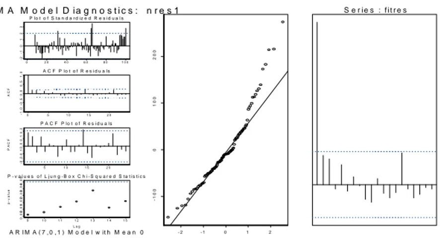
For the data set we investigated, the de-trended load (for both on peak and off peak segments) followed ARIMA(7,0,1) for each partition. This is consistent with the study of Dupacova, Growe-Kuska and Roemisch (2000) who examined hourly loads (which can be considered as high frequency data) and concluded that SARIMA(7,0,9)×(0,1,0) was an appropriate model for hourly loads.
In Figure 2, we provide plots of the remaining residuals, the autocorrelation, partial autocorrelation functions, p-values of Ljung-Box statistics, and qq-normal plot of residuals. Both ACF and PACF of residuals are within the bounds and Portmanteau test validates this with the qq-normal plots as well.
These diagnostics validate the sufficiency of the approach.
0 2 0 4 0 6 0 8 0 1 0 0
-2-10123
P lo t o f S t a n d a r d iz e d R e s i d u a l s
0 5 1 0 1 5 2 0
-1.0-0.50.00.51.0
ACF
A C F P lo t o f R e s i d u a ls
5 1 0 1 5 2 0
-0.2-0.10.00.10.2
PACF
P A C F P lo t o f R e s i d u a ls
9 1 0 1 1 1 2 1 3 1 4 1 5
L a g
0.000.010.020.030.040.05
p-value
P - v a l u e s o f L j u n g - B o x C h i - S q u a r e d S t a t is t i c s
M A M o d e l D ia g n o s t i c s : n r e s 1
A R I M A ( 7 , 0 , 1 ) M o d e l w it h M e a n 0 - 2 - 1 0 1 2
-1000100200
S e r i e s : f i t r e s
Figure 2: Diagnostic Checking of ARIMA(7,0,1) Fitting of De-trended Load Series, Quantile-quantile Plot, and ACF of Remaining Residuals
3.1.1 Alternative Load Models
Another load model is based on historical load with drift as well as random noise, which captures cyclicality and seasonality commonly observed in load.
1
, 0 , 1 , , ,
y y
d s s s d s d s
L =α +α L − +ε (Demand Model 2) ,
where y denotes a year for which the load forecast is being made. Given the success of model 1 we used ARIMA (p,d,q) to model the noise. Using ten years of historical load data, once again we find that p=7, and d=0 or 1 and q=1or 7 provide well behaved auto-correlation and partial-autocorrelation functions and Portmanteau test results.
Neither “Demand Model 1” nor “Demand Model 2” use temperature as an explanatory variable.
However temperature and humidity are often considered as explanatory variables (Feinberg (2002)). In Arizona (the state for which our forecasts are valid) temperature is a more dominant factor. Using this factor another load model we investigate is as follows.
1 1
, 0, 1, , 2, , ,
y y y
t s s s t s s t s t s
L = +α α T − +α L− +ε (Demand Model 3)
This load model uses “high” temperature for the previous year to predict on-peak loads and “low”
temperature for the previous year to predict off-peak loads. Because of high lag values and persistence of residual load we investigated GARCH (p,q), [1,5]p∈ ,and [1, 2]q∈ . Based on Schwarz’s Bayesian criterion (SBC) we have chosen p=q=1 and observed statistically significant coefficients. The autocorrelation function of standardized squared errors suggested serial uncorrelatedness, implying that
the model of the error term has captured persistence in the model. For the above model we have also tried ARIMA (p,d,q). Again we obtained the same p, d, q values that we observed in “Demand Model 2.”
Decision makers using the DASH model may use any of these alternatives to forecast demand during the study period.
3.2 Modeling Electricity Forward Prices
This part of the DASH model forms the core of our scenario generation procedures. The inputs we use are the forward prices for the preceding year, together with recent trends in the market. Let us first focus on the forward prices for the preceding year. These are available as hourly quotes which we transform into “on-peak” and “off-peak” average prices. We have the following format for the prices:πτκe, where πis the price, and ,τ κ and e denote the contract week, delivery week and segment, respectively. Here, the range of indices are:τ =1, 2,...52, κ ={1, 2,...,N},e∈{on off, }, N denotes the last week in which delivery will happen. For example, π1,8,onis the price ($/MWh) on January 7th (i.e. end of week 1) for on-peak power delivered starting on March 1st (for the entire month of March). However we use “returns” to predict prices; that is, rτ κ, ,e =(πτ+4, ,κe−πτ κ, ,e) /πτ κ, ,e. Since the index τ reflects a index for weeks, the subscript τ + 4 denotes a period that is four weeks removed from period τ . Assuming that there are four weeks in a month, the return rτ κ, ,e denotes the relative change in price during the month starting in week τ .
There are two important reasons behind this choice (of using returns over prices). First, this approach allows us to treat different power contracts (associated with different months) with the same scenario tree, thus reducing the complexity of modeling the evolution of prices associated with each type of contract. We have empirically verified that it is the interval of time between contract and delivery that is important for modeling returns, and not the actual contract. Hence the same scenario tree remains a valid representation of returns for alternative contacts. Secondly, the econometrics literature recommends that “returns” are better for predictive purposes because empirical evidence suggests that they appear to have better properties (e.g. stationarity) from a computational point of view (Taylor (1986)).
A discrete scenario tree may now be formed by grouping returns into subsets for each period (i.e.
month), and modeling the return process as one that allows probabilistic transitions from one subset to another, over time. In order to maintain computational tractability, we consider only two subsets in each period: “High” and “Low” return states. Thus, the resulting scenario tree can be represented by a binary tree in which the returns can assume “High” or “Low” values over the course of the decision process.
To assign “High” and “Low” values for the return states, we adopt a sampling-based procedure that is guided by recent observations of the return series. The nominal value that we assign to each state (“High” or “Low”) is the median of the corresponding group for that period. However, without accommodating extreme values, the scenario tree (and consequently the decisions themselves) overlooks extreme events, thus opening up the possibility for catastrophic losses. We will of course, include some loss constraints within the decision model, but in the absence of extreme scenarios, such constraints can only have limited impact. Accordingly, we use a combination of medians and extreme values (“Min”
and “Max”) to assign values to the High and Low states. The precise manner in which we choose one or the other depends on a heuristic guided by market conditions prior to running the model. Finally, the formation of the scenario tree requires a specification of transition probabilities between nodes which represent information states. Recall that our scenario tree is binary, and hence there are only two probabilities that need to be specified. In the event that our heuristic produced two nodes that are represented by medians (High and Low respectively), then we simply use equal conditional probabilities for these two transitions. On the other hand, if the heuristic produces an extreme value for one path, and a median for the other, then we associate a conditional probability of ¼ for the extreme value, and ¾ for the median value. Our heuristic does not produce two extreme values from any node, and hence this possibility is not considered.
The above process creates a binary scenario tree for the return series, which is then used to create prices scenarios that are used within the stochastic programming model described in the following section.
3.3 Modeling Gas Forward Prices
The process used to model gas forward prices is similar to the process described in the previous subsection (on electricity forward prices). We will also assume that the returns for gas and electricity are perfectly correlated so that a scenario obtained from the electricity forwards returns tree generates a similar scenario from the gas forwards return tree.
3.4 Modeling Electricity Spot Prices
Recall that the forward price process is discretized on a monthly basis. However, spot prices must be modeled on a different time scale. As discussed earlier, on-peak and off-peak spot prices will be modeled on a daily basis, with the understanding that they will be correlated with an appropriate forward price scenario. As with the forwards, we resort to modeling the return series of spot prices.
The spot prices during a delivery month are generated from the following formulation (of spot returns): re d, , ,p τ ω =re t, ,fω+σe t, zd t, ,ω, where ωis the node number of the forward scenario tree, σe t, is the standard deviation of spot returns which changes from delivery month to delivery month, and re t, ,fωis the daily equivalent of the forward return (rt t, 1,+ e) on node ω for month t. The quantity z represents a standard normal random variate. Here σe t, may be interpreted as the volatility associated with on-peak and off-peak returns during month t and are estimated using a GARCH (Generalized Auto Regressive Conditional Heteroskedasticity) model (Bollerslev (1986)). Because the expectation of spot market prices may be assumed to equal the expected forward prices (Hull (1997)), the above relationship between spot and forward returns captures both the first as well as second moments of the spot price process.
4 THE DECISION MODEL
The DASH model may be classified as a multi-stage stochastic integer program which recommends forward decisions on a here-and-now basis, whereas, the operational decisions (generation, spot market activity etc.) are used to evaluate the viability of the portfolio. In this sense, the generation and spot market decisions are adaptive (i.e. wait-and-see), and allow us to compute medium (six months to a year) decisions without being mired in daily (here-and-now) details.
In formulating the stochastic program, all decision variables and parameters are dependent on the scenario. However, in the interest of simplifying the notation we have suppressed this dependence below. We remind the reader that all forwards variables will be required to satisfy the non-anticipativity requirements of stochastic programming (Birge and Louveaux (1997)). The formulation is presented in two parts: the financial problem and generation costing problem.
4.1 The Financial Problem Scenario Independent Parameters
α : Max liquidity limit coefficient;
T : Number of periods;
ε : {on-peak, off-peak};
H : Hours of one on/off peak segment, e H =16h for e=on peak, and 8h for e=off peak; e
YL te
0 : Power forward in long position for delivery period t, peak e held initially;
YS te
0 : Power forward in short position for delivery period t, peak e held initially;
YG t
0 : Gas forward for delivery period t held initially;
Scenario Dependent Parameters
PPτte : Price of power forward for delivery period t, peak e(on/off peak) at contract period τ;
PGτt : Price of gas forward for delivery period t, at contract period τ;
Scenario Dependent Decision Variables
FPτte : Power forward for delivery period t, peak e (on/off peak), signed at contract period τ (positive for long position, negative for short position);
+
FPτte : Power forward in long position for delivery period t, peak e (on/off peak), signed at contract period τ;
−
FPτte : Power forward in short position for delivery period t, peak e (on/off peak), signed at contract period τ;
FGτt : Gas forward in long position for delivery period t, signed at contract period τ;
YPτte : Power forward for delivery period t, peak e held at period τ(positive for long position, negative for short position);
YLτte : Power forward in long position for delivery period t, peak e held at period τ;
YSτte : Power forward in short position for delivery period t, peak e held at contract period τ; YGτt : Gas forward for delivery period t held at contract period τ;
ZP : Total power forward cost for delivery period t, peak e; te
ZG : Total gas forward cost for delivery period t; t
Scenario Dependent Constraints
FP FP FP
te te te
τ = τ+ − τ− τ∈{1,,T},t∈{τ,,T},e∈ε; (1)
YP YL YS
te te te
τ = τ − τ τ∈{1,,T},t∈{τ,,T},e∈ε ; (2) + +
= −
FPte YL te
YLτte (τ 1) τ τ∈{1,,T},t∈{τ,,T},e∈ε (3) (Power forward balance in long position at period τ);
+ −
= − FPte
YS te
YSτte (τ 1) τ τ ∈{1,,T},t∈{τ,,T},e∈ε (4) (Power forward balance in short position at period τ);
FG t YG t
YGτt = (τ −1) + τ τ∈{1,,T},t∈{τ,,T},e∈ε (5) (Gas forward balance at period τ);
YL te T te t
FP T
t ( 1)
] , [ ]
,
[ ∑ −
≤ ∈
∑ +
∈τ τ α τ τ
τ ∈{1,,T},e∈ε (6) (Max liquidity limit for long position);
YS te T te t
FP T
t ( 1)
] , [ ]
,
[ ∑ −
≤ ∈
∑ −
∈τ τ α τ τ
τ∈{1,,T},e∈ε (7) (Max liquidity limit for short position);
[1, ]
te te te e
t
ZP PP FP Hτ τ
τ∈
=
∑
t∈{1,,T},e∈ε (8) (Total power forward cost for delivery period t, peak e);∑
∈=
] , 1 [ t
t t
t PG FG
ZG
τ τ τ t∈{1,,T} (9) (Total gas cost for period t);
Constraints (1-5) constitute balance constraints (dynamics). Constraints (6-7) provide a way control the extent to which a portfolio is allowed to change from one period to the next period. These constraints help avoid speculation, thus limiting risk exposure. The lower the value ofα , the tighter the control is on the trajectory allowed by the model. The costs associated with the forwards decisions are captured in (8-9). Finally, there are two important factors required in specifying the financial problem.
• Non-anticipativity constraints require that scenarios which share the same history until period t should be associated with decisions which have the same values until period t. These linear constraints couple decisions from different scenarios, thus allowing a well hedged plan.
• The objective function for the financial problem maximizes expected profits associated with the portfolio. In calculating the profits, we accommodate the generation cost, which is computed via the model discussed next.
4.2 The Generation Problem
With each scenario we associate a series of generation problems and each generation problem models a period of power production. Thus for any scenario, there will be the same number of generation problems as there are periods in the financial model. In this formulation, the generation and spot market variables are allowed to be adaptive. As before, the notation suppresses the dependence on scenarios.
Scenario Independent Parameters
I : The set of generators;
J : The number of segments in period t; in a month consisting of 28 days, there are 56 segments; t
d : Index of days.
( )
j d : Set of indices of segments in day d.
ML : Maximum acceptable daily loss;
Gas : The set of gas generators;
Coal : The set of coal generators;
Nuc : The set of Nuclear generators;
p(j) : Peak status(on/off) of segment j;
P : Regulated power price;
CP : Coal price for period t; t
NP : Nuclear fuel price for period t; t
Qi : Maximum generation capacity of generator i;
q : Minimum generation capacity of generator i; i
Li : Minimum up time requirement for generator i;
l : Minimum down time requirement for generator i; i
i( )
F x : Consumption of fuel for generation of x due to generator i;
Scenario Dependent Parameters
Witj : Scheduled outage (
Witj=0, if outage is scheduled in period t, segment j for generator i; 1, otherwise);
ωitj : Forced outage (
ωitj=0, if outage is forced in period t, segment j for generator i; 1, otherwise);
PStj : Price of power in spot market in period t, segment j;
D : Electricity demand in period t, segment j; tj
Scenario Dependent Decision Variables
G : Total generated power in period t, segment j; tj
Gitj : Power generated by generator i in period t, segment j;
Uitj : Decisions about turning on/off generator i in period t, segment j (binary variables);
SPtj : Power exchanged with spot market in period t, segment j (positive for purchase, negative for sale);
YG : Consumption of gas in period t, segment j; tj
YC : Consumption of coal in period t, segment j; tj
YN : Consumption of nuclear fuel in period t, segment j; tj
Ctj : Total generation cost in period t, segment j;
Scenario Dependent Constraints
Dtj Gtj SPtj
YPtte+ + = t∈{1,, },T j∈J et, = p j( ) (10) (Demand-generation- forward - spot relationship);
t tj j J
YG YG
tt =
∑
∈ t∈{1,,T} (11) (Gas consumption for period t);∈
∑
=
Gas i
itj i
tj F G
YG ( ) t∈{1,,T}, j∈Jt (12) (Gas consumption for period t, segment j);
( )
tj i itj
i Coal
YC F G
∈
=
∑
t∈{1,,T}, j∈Jt (13) (Coal consumption for period t, segment j);( )
tj i itj
i Nuc
YN F G
∈
=
∑
t∈{1,,T}, j∈Jt (14) (Nuclear fuel consumption for period t, segment j);t
tj t tj t tj
t
C ZG NPYN CPYC
= J + + t∈{1,,T}, j∈Jt (15) (Generation cost for period t, segment j)
Gitj I tj i
G ∑
= ∈ t∈{1,, },T j∈Jt (16) (Total generated power at period t, segment j);
Uitj Qi Gitj Uitj
qi ≤ ≤ i∈I t, ∈{1,, },T j∈Jt (17) (Operating range for each generator);
τ Uit j
Uit
Uitj − , −1≤ i∈I t, ∈{1,, },T j∈Jt,τ∈ +{j 1,,min(j L+ −i 1,|Jt|)}
(Minimum up-time requirement); (18) τ
Uit Uitj
j
Uit − − ≤1− 1
, i∈I t, ∈{1,, },T j∈Jt,τ∈ +{j 1,,min(j l+ −i 1,|Jt|)}
(Minimum down-time requirement); (19) Witj
Uitj ≤ i∈I t, ∈{1,, },T j∈Jt (20) (Scheduled outage);
itj
Uitj ≤ϖ i∈I t, ∈{1,, },T j∈Jt (21) (Forced outage);
( ) ( )
[( tj tj tj) p j tj] te 0 ,
j j d e
D P SP PS H C ZP ML d
∈ ∈ε
− − − + ≥ ∀
∑ ∑
(22)(Max daily loss constraint).
The max-daily loss constraint is imposed in order to provide a measure of risk control on the decisions.
Note that the estimated cost of gas forwards (Ctj) is prorated according to the number of segments in the period/month (see (15)). There are more accurate ways to allocate the cost of gas forwards to each segment, but variables introducing usage-based allocation for each segment results many more coupling variables between the financial and generation problems, and that would limit the ease with which these submodels may be decomposed within an algorithm. Accordingly, we have adopted the formulation of
(15) and (22). Although (22) is a financial constraint, it is included within the generation model.
Because spot market prices and demands are modeled on a daily basis, it is best to incorporate risk control on a daily basis, and hence this constraint appears in the generation model. However the model may become infeasible in instances in which the target ML is unattainable. In such instances it may be recommended that the user include such a measure within a penalized objective function for the generation problem.
Finally, we discuss the objective function for the generation problem. This function reflects the “cost”
of spot market activity, as well as the cost of power generation. This objective is similar to that used in Takriti, Krasenbrink and Wu (2000). The complete objective function for the DASH model maximizes discounted expected profit where the expected production cost is obtained from a unit commitment model run under alternative scenarios.
The alternative time indexes used in the above formulation results in multi-granularity model with the financial decisions being made on a monthly time index, and the generation decisions being indexed by segments which are either eight or sixteen hours long.
5 A NESTED COLUMN GENERATION DECOMPOSITION STRATEGY
The stochastic programming model presented in the previous section is a very large scale optimization problem. Fortunately, the model is amenable to solution using decomposition techniques. This discussion is best motivated by studying the structure of the DASH model.
5.1 Here-and-now Problem Embedded with Wait-and-see Problems
In section 4, the DASH model was presented in terms of its two main sub-models: the financial model and the generation model. The financial decisions in this model are made on monthly basis. In each decision period, forwards positions are decided for each of the future delivery months. As the market evolves in the future, these positions will be rebalanced in order to react to changes in the market.
Because the forwards decisions are made before forwards prices are realized, they should be treated as here-and-now decisions. Thus forwards scenarios will provide monthly evolution of prices and the here- and-now (financial) decisions will be required to be non-anticipative with respect to the forward prices
scenario tree. We should reiterate that the forward prices refer to multiple stochastic processes including on-peak/off-peak power, and gas.
Note that the focus of the DASH model is forwards decisions, with the generation costs merely providing the basis for economical decisions. Unlike the financial decisions, the generation decisions are assumed to be made on a segment-by-segment basis (i.e. 16 hour on-peak, and 8 hour off-peak). That is, for each forwards scenario, generation decisions follow the evolution of load and spot prices during each month of a given scenario. This suggests a wait-and-see (adaptive) approach for the generation decisions. Nevertheless, it should be noted that if there are two scenarios that have the same partial data history (i.e. load, forwards and spot prices), then the generation history associated with these scenarios should also be the same. This implies that the generation decisions should also be required to satisfy non-anticipativity constraints. Given that there are a large number of segments within the model (e.g.
336 per scenario in a six month planning horizon), imposing non-anticipativity requirements for each generator would make the entire approach far too complex for even a decomposition approach such as the one developed in this paper. Fortunately, we are able to obtain non-anticipativity of generation decisions by imposing a specific relationship between the period index t (e.g. months), and the segment index j. Specifically, we assume that there is negligible loss by decoupling the generation model associated with period t (i.e. Month t) and that associated with period t+1 (Month t+1). Under this assumption, it is easily seen that a generation-costing model for any period (month) cannot be affected by data in the future. Hence, decoupling the generation problems, together with non-anticipativity of the forwards decisions, ensures that two scenarios that have the same partial data history will also have the same partial generation history. That is, non-anticipativity of the generation decisions is a consequence of our decoupling assumption, and the non-anticipativity of forwards decisions. The resulting structure is therefore one that involves a multi-stage here-and-now stochastic program that has a sequence of large wait-and-see MILP embedded within it. This structure turns out to be quite useful for decomposition because the unit commitment model, an MILP, is much easier when treated as a wait-and-see problem, than as a here-and-now problem (Takriti, Krasenbrink and Wu, (2000), Nowak and Romisch, (2000)).
In order to give the reader a sense of the magnitude of each scenario problem, the financial decisions involve T(T-1)/2 for each of the following types of forwards: on-peak electricity, off-peak electricity and gas. This certainly seems manageable for reasonable values of T (e.g. T=6 or 12). For the generation
problem, each day corresponds to two segments (on-peak and off-peak), each served by |I| generators.
Hence for a month-long unit-commitment model involves 56 segments, and hence 56|I| binary variables.
By aggregating some of the generators, it is possible to solve such problems with reasonable computational effort. However, if the number of generators is large, then, it may be more convenient to solve the unit-commitment problems on a week-by-week basis.
5.2 Nested Column Generation Decomposition Strategy
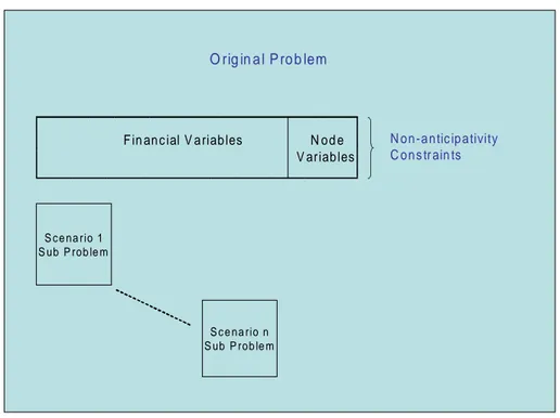
Our approach decomposes the stochastic program into three interrelated optimization problems which are motivated by a nested column generation (i.e. Dantzig-Wolfe) decomposition strategy. The algorithm is best motivated by studying the structure of the model. Figure 3 illustrates the original DASH model which consists of non-anticipativity constraints and all scenario sub-problems. Figure 4 summarizes the structure of each scenario problem, which consists of complete forwards dynamics and all generation problems. The forwards positions that are ultimately realized (on a delivery date) appear in the generation model as shown in Figure 4. Given that both Figures 3 and 4 depict block-angular matrices, it is natural to consider an algorithm in which column generation is carried out in a nested manner; that is, we develop a non-anticipativity master problem (see Figure 5) whose responsibility is to seek non-anticipative forwards decisions by choosing convex combinations of columns that represent each scenario. Similarly, Figure 6 depicts a master program for any scenario, and the columns generated here represent forwards positions for the scenario. These positions are proposed by the generation problem. Thus, the nested column generation approach adopted here involves interactions between three problems described below.
1. We use a non-anticipativity master problem to enforce non-anticipativity restrictions. Each scenario is represented by a collection of columns in this problem, and its goal is to find a convex combination of columns of each scenario that also satisfy non-anticipativity restrictions.
Initially, a Phase I problem is solved to obtain a feasible solution to this problem. We note that the objective function coefficient for each column in this problem represents the total profit under a particular scenario of forward prices, spot prices, and electricity demand.
2. Given the price for achieving non-anticipativity from the master problem described above, mid- level coordinating problem (scenario master problem) is formulated to make the best forward
decisions for each scenario. This is essentially the same formulation as the financial problem described in section of decision model. However, the summation of forward decisions for a certain delivery period is once again represented via a convex combination of forward columns that are generated by the corresponding generation problem where the summation of forward decisions appear in the demand constraint (8). Here, we decompose the whole embedded generation problem (wait-and-see) into several generation problems, one for each delivery period (month).
3. Finally, the lowest level problem (generation problem), which generates the aggregation (i.e.
summation) of forward columns for the higher levels, consists of a series of unit-commitment problems. As with the second level coordinator, this problem assumes that the scenario is given, and a series of deterministic instances of the unit commitment problem are solved. The prices of forwards in this problem are modified by the dual prices from forward balance constraints in the mid-level coordinator (scenario master problem).
A few remarks regarding the advantages of our algorithm are in order. First, the nested approach allows us to maintain modularity, so that generation costing and financial decision are performed by coordinated, yet independent models. Moreover, such modularity promotes the ability to use a distributed computing environment, which has its own advantages (scalability, reliability etc.). Finally, we observe that in cases where a succession of instances are solved, with some changes in the probability measure, the non-anticipativity master problem can be warm-started using previously generated columns, thus allowing efficient re-solves.
N o n -a n tic ip a tivity C o n s tr ain ts F in an c ial V a riab les N o d e
V ariab les
S c e na rio 1 S ub P rob le m
S c e na rio n S ub P rob le m
O rig in a l P ro b lem
Figure 3: Original Problem Structure
G eneration Problem 1
G eneration Problem m D elivery D ate F orw ards
Pos ition
C om plete F orw ards D ynam ic s
S cen ario S ubp ro blem
Figure 4: Scenario Sub-problem Structure
Non-anticipativity Constraints Columns from
Scenario 1 Columns from
Scenario n
State Vector Formulation
Convexity Constraints
Non-anticipativity Master
Figure 5: Non-anticipativity Master Structure
C o lu m n s for D e live r y D a te F o rw a rds P o s itio n
C o n ve xit y C o ns tra ints
F orw a rds D yn am ic s in C o ntra c t M on ths (N o n -d eliver y M on ths )
F orw a rds D yn am ic s A t D e live r y M o nth F orw a rds V ariab les (S tate
a nd D ec is io ns )
S cena rio M aster
Figure 6: Scenario Master Structure
In order to solve DASH problem with the above decomposition strategy, we apply CPLEX 7.0 to implement the nested column generation decomposition algorithm. The CPLEX Barrier Optimizer is used to solve Non-anticipativity master problem, and the Simplex Optimizer to solve the Scenario Master Problem. It is well known (see Carpenter, Lustig, and Mulvey (1991)) interior point methods are superior to the Simplex method for stochastic programs with the split variable formulation, as in our case. These are very large, sparse problems. The generation problem is a mixed-integer program, and we use CPLEX Mixed Integer Optimizer to solve it.
6 EXPERIMENTAL RESULTS
The experiments reported here are intended to investigate the robustness of decisions provided by the DASH model. In order to do so, we study the performance of DASH decisions in three settings: a) a back-casting exercise in which the decisions are evaluated with respect to the data observed during the first half of 2001, b) a simulation exercise in which the DASH decisions were evaluated when scenarios were generated from an extended scenario tree which involved four branches (instead of two) at each node, and c) a simulation exercise in which the price models are completely independent of the scenario tree models used by DASH. These price models are described subsequently in this section. In any event, our intent is to test the performance of DASH under various “stresses” so that any weaknesses can be identified.
For comparative purposes, our tests will be carried out against a benchmark known as the “fixed-mix”
policy, which is relatively common in this industry. The “fixed-mix” strategy may be described as follows.
On any contract date, an appropriate hedging position for a future delivery date (month) is one that is determined according to the following strategy. Make a prediction of expected demand and expected capacity for the delivery month. If expected demand exceeds expected capacity, then assume a long position for forwards in that delivery month, and the quantity of this transaction should be a fraction
“f” of the difference. On the other hand, if expected capacity exceeds expected demand, then one should assume a short position for forwards in the delivery month being considered. Once again, the quantity associated with this transaction should be a fraction “f” of the difference.
One can devise several variations on this scheme. For instance, instead of using expected demands and capacities, one may use scenarios to determine scenario-dependent strategies, and then use some weighted averaging to determine the exact mix. For our experiments we only tested the basic scheme outlined in the previous paragraph. However, we ran our simulations using several values of the fixed- mix fraction f, including 0, 0.1, 0.2, 0.3 and 0.4. We should also note that the simulations used here incorporate greater details on generation capacities than that used within the DASH decision model.
6.1 The Backcasting Experiment
As outlined in the introduction, this experiment covers a five month operating period from January 2001 through May 2001, with hedging decisions being made once each month. The decisions at the beginning of each month are, of course, made prior to observing the markets. Once the transactions are carried out, no portfolio changes are allowed for the rest of the month. During this period, we run a generation costing simulation based on weekly unit-commitment and calculate the actual weekly profit. There are two steps for this procedure. In the first step, we forecast power demands and spot prices for the coming week, and run a weekly generation problem based on forwards decisions for current period. In step 2, we calculate the actual profit based on the scheduled generation, actual demands and spot prices. Following this procedure, we can simulate the actual profits week by week during the current month. At the start of the next month, we once again use the fixed-mix policy to obtain the newly rebalanced positions, and the process resumes again. For all runs reported here, we used an initial position of forwards amounting to 15% of the averaged electricity load for a certain period. The electricity market data for our study reflects prices at Palo Verde, AZ, whereas, the gas market prices reflect data from Henry Hub, LA. The hedging decisions made in this study allowed delivery dates up to six months in the future. For the sake of this study, transaction costs were not included, although such calculations are easily accommodated within a simulation. Moreover, since all rules carry out the same number of transactions, the difference in transactions costs between the different policies can be ignored. Finally, a word is about costs and revenue calculations. Costs/revenues are calculated using the unit commitment (generation) model which includes spot market and forwards activity. Thus revenues are accounted for in a delivery month only.
Fixed-mix Profit Fractions
0.80 0.85 0.90 0.95 1.00 1.05 1.10
1 2 3 4 5
Month
fix_m0%
fix_m10%
fix_m20%
fix_m30%
fix_m40%
Figure 7: Comparisons between Fixed-mix Strategies
The experiments reported in this study are based on data obtained from Pinnacle West Capital. In order to maintain confidentiality of the data, we will report performance in terms of fractions, with the best policy assuming the value of 1. Figure 7 is based on outputs that showed that using f = 0.1 provided the most profitable fixed-mix strategy. Note that although some other fractions appear to be competitive during certain months, using f = 0.1 provides the overall winner among the fixed-mix strategies.
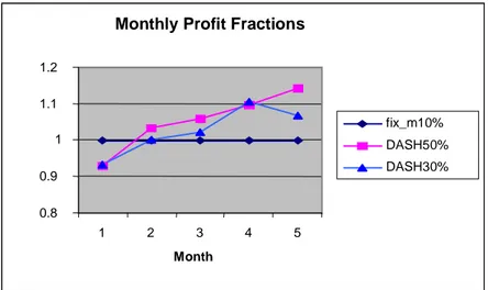
Next we proceed to experiments with the Stochastic Programming approach. These experiments were run with the same data as above, except that the fixed-mix hedging rule was replaced by decisions from the stochastic programming model. During each month (January 2001 through May 2001), we run the stochastic programming model once. As before, decisions are made before observing market prices at Palo Verde, AZ and Henry Hub, LA. The planning period used within the decision model was five months long (i.e. T = 5). Hence as in the previous experiments, delivery dates of six months in the future were permitted in the model. Thus, the experimental setup, and data are exactly the same as in the previous study, and this permits comparisons between hedging decisions from stochastic programming and those from the fixed-mix rule.
Monthly Profit Fractions
0.8 0.9 1 1.1 1.2
1 2 3 4 5
Month
fix_m10%
DASH50%
DASH30%
Figure 8: Comparing DASH with Fixed-mix Strategy (Backcasting Data)
In Figure 8 we use the best fixed-mix strategy (f = 0.1) as the basis for our comparisons. We made two series of runs with the DASH decisions: one using α= 0.3 (i.e. 30% change allowed in the portfolio from one month to the next), and another series of runs using α= 0.5 (i.e. 50% change allowed in the portfolio from month to month). The motivation for such controls was discussed earlier in the paper (see section 4.1). In any event, both series of DASH runs perform significantly better than the best fixed- mix strategy. It turns out that the series of revenues for α= 0.5 exceeds that for the best fixed-mix strategy by approximately 7% per month, on average. This is a significant advantage in favor of the DASH model.
Before closing this subsection, we should comment on a certain initialization bias that results from restrictions imposed by the initial portfolio. Recall that when we allow a 50% change allowed in the portfolio from month to month (α= 0.5), it takes about 2 months for the effect of the initial portfolio to wear off. It is therefore appropriate to focus our attention on the performance of DASH (with α= 0.5) for months 3, 4 and 5. Similarly, when α= 0.3, the output for months 4 and 5 are critical. Thus if we set aside the initialization bias, the performance of the DASH model for the period March – May 2001 is clearly superior to all tested fixed-mix strategies.
6.2 Results of Experiments with Synthetic Scenarios from an Extended Scenario Tree
In order to test the robustness of the decisions provided by the DASH model, we created synthetic scenarios and tested the decisions provided by the model against these scenarios. In conducting this
phase of our experiments, we did not re-optimize to allow DASH to adapt to the observed (synthetic) scenario; instead, we used the decisions obtained from the back-casting experiment, and applied those to the synthetic scenarios. Hence the gains reported here are lower bounds on potential improvements. In these experiments, we follow the same simulation procedure as the one in back-casting experiment.
The synthetic scenarios of this section were created in two steps. First, we create a series of forward prices from a discrete-time stochastic process with each time step reflecting the passage of a month.
During each month, we draw a random number representing a particular outcome of forward prices. We allow four such outcomes in any month: {Max, High-Median, Low-Median, Min}. The values for these quantities are obtained from historical data as described in section 3.2, and the probability of these outcomes is assumed to be {1/8, 3/8, 3/8, 1/8}. Note that over a five month period, we can create a total of 1024 scenarios. For the purposes of our tests, we generate 30 scenarios, against which the model is tested. For each of these scenarios, we also generate spot market prices, and loads. The latter are created in the same manner as described in section 3.
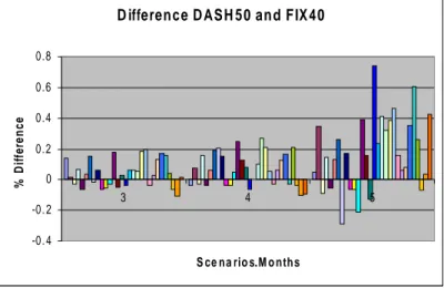
Due to the initialization bias in the first two months (see the last paragraph of section 6.1), the comparison we report pertains to months 3, 4 and 5. This comparison involves the DASH model (α= 0.5) and the fixed-mix strategy using f = 0.1. Figure 9 depicts the fraction of differences (i.e. (DASH – Fixed-Mix/Fixed-Mix)) over all 30 scenarios, for months 3, 4 and 5. Upon examining this figure, it is clear that DASH is the winner over most scenarios, with the magnitude of wins being significantly higher than the magnitude of losses. A summary of Figure 9 in terms of win-loss statistics is provided in Table 1.
The win-loss advantages in favor of DASH are unmistakable. Moreover, these results may underestimate the gains because the DASH model was not re-optimized based on observations of the evolving (synthetic) scenario.
Difference Dash50 and Fix10
-0.4 -0.2 0 0.2 0.4 0.6 0.8 1 1.2
3 4 5
Scenerios.Months
Figure 9: Comparing DASH (α =0.5) with Fixed-mix Strategy (f=0.1)
Table 1: Win-Loss Statistics with scenarios from extended tree
Month\Statistic
Wins-Losses for DASH
Average Size of Wins
Average Size of Losses
3 22-8 3.29% 4.70%
4 19-11 11.19% 6.82%
5 19-11 21.68% 12.91%
6.3 Generating Synthetic Scenarios using Alternate Price Models
While the results of the previous subsection are very encouraging, it remains to be seen how the model might perform under realistic scenarios that are not related to the scenario tree used to create the DASH decisions. In order to do so, we modeled the price processes (gas, electricity forwards and spot) directly, rather than modeling “returns” as in formulating the scenario tree (see section 3). These price models are similar in spirit to studies by Eydeland and Geman (1998), but as one might expect, our prices create scenarios. The details are discussed below, and are significantly different from previous work.
6.3.1 Gas Spot Pricing
Because gas generators are usually the last ones to be dispatched for merit ordered electricity generation, the marginal cost of electricity reflects gas prices. Hence, it is natural to first model gas spot prices, followed by gas spot price scenarios, and then electricity spot price scenarios. The reader may recall that the DASH model does not allow activities in the gas spot market, and the entire reason for studying gas