doi: 10.3389/fmars.2019.00138
Edited by:
Maria Snoussi, Mohammed V University, Morocco
Reviewed by:
Edward Hanna, University of Lincoln, United Kingdom Horst Machguth, Université de Fribourg, Switzerland Andrew John Sole, The University of Sheffield, United Kingdom
*Correspondence:
Fiammetta Straneo fstraneo@ucsd.edu
Specialty section:
This article was submitted to Ocean Observation, a section of the journal Frontiers in Marine Science
Received:14 November 2018 Accepted:05 March 2019 Published:29 March 2019
Citation:
Straneo F, Sutherland DA, Stearns L, Catania G, Heimbach P, Moon T, Cape MR, Laidre KL, Barber D, Rysgaard S, Mottram R, Olsen S, Hopwood MJ and Meire L (2019) The Case for a Sustained Greenland Ice Sheet-Ocean Observing System (GrIOOS).
Front. Mar. Sci. 6:138.
doi: 10.3389/fmars.2019.00138
The Case for a Sustained Greenland Ice Sheet-Ocean Observing System (GrIOOS)
Fiammetta Straneo1* , David A. Sutherland2, Leigh Stearns3, Ginny Catania4, Patrick Heimbach4, Twila Moon5, Mattias R. Cape6, Kristin L. Laidre7, Dave Barber8, Søren Rysgaard8,9,10, Ruth Mottram11, Steffen Olsen11, Mark J. Hopwood12and Lorenz Meire10,13
1Scripps Institution of Oceanography, University of California, San Diego, La Jolla, CA, United States,2Department of Earth Sciences, University of Oregon, Eugene, OR, United States,3Department of Geology, University of Kansas, Lawrence, KS, United States,4Oden Institute for Computational Engineering and Sciences and Jackson School of Geosciences, University of Texas at Austin, Austin, TX, United States,5National Snow and Ice Data Center, Cooperative Institute for Research in Environmental Sciences, University of Colorado, Boulder, Boulder, CO, United States,6School of Oceanography, University of Washington, Seattle, WA, United States,7Polar Science Center, Applied Physics Laboratory, University of Washington, Seattle, WA, United States,8Centre for Earth Observation Science, Department of Environment and Geography, University of Manitoba, Winnipeg, MB, Canada,9Arctic Research Centre, Aarhus University, Aarhus, Denmark,10Greenland Climate Research Centre, Greenland Institute of Natural Resources, Nuuk, Greenland,11Danish Meteorological Institute, Copenhagen, Denmark,12GEOMAR Helmholtz Centre for Ocean Research Kiel, Kiel, Germany,
13NIOZ Royal Netherlands Institute of Sea Research and Utrecht University, Yerseke, Netherlands
Rapid mass loss from the Greenland Ice Sheet (GrIS) is affecting sea level and, through increased freshwater and sediment discharge, ocean circulation, sea-ice, biogeochemistry, and marine ecosystems around Greenland. Key to interpreting ongoing and projecting future ice loss, and its impact on the ocean, is understanding exchanges of heat, freshwater, and nutrients that occur at the GrIS marine margins.
Processes governing these exchanges are not well understood because of limited observations from the regions where glaciers terminate into the ocean and the challenge of modeling the spatial and temporal scales involved. Thus, notwithstanding their importance, ice sheet/ocean exchanges are poorly represented or not accounted for in models used for projection studies. Widespread community consensus maintains that concurrent and long-term records of glaciological, oceanic, and atmospheric parameters at the ice sheet/ocean margins are key to addressing this knowledge gap by informing understanding, and constraining and validating models. Through a series of workshops and documents endorsed by the community-at-large, a framework for an international, collaborative, Greenland Ice sheet-Ocean Observing System (GrIOOS), that addresses the needs of society in relation to a changing GrIS, has been proposed.
This system would consist of a set of ocean, glacier, and atmosphere essential variables to be collected at a number of diverse sites around Greenland for a minimum of two decades. Internationally agreed upon data protocols and data sharing policies would guarantee uniformity and availability of the information for the broader community. Its
development, maintenance, and funding will require close international collaboration.
Engagement of end-users, local people, and groups already active in these areas, as well as synergy with ongoing, related, or complementary networks will be key to its success and effectiveness.
Keywords: Greenland, ice sheet, ocean, observing system, glacier, atmosphere
INTRODUCTION
Scientific Rationale for a Greenland Ice Sheet-Ocean Observing System
Rapid mass loss from the Greenland Ice Sheet (GrIS) has raised interest in glacier–ocean interactions for three main reasons.
First, melting at the marine margins of Greenland glaciers has emerged as a potential trigger of the observed dynamic ice loss (roughly half of the total ice loss) with important consequences for sea level rise. Second, increased freshwater discharge from the GrIS has the potential to impact global climate by affecting the Atlantic Meridional Overturning Circulation. Third, by altering nutrient fluxes, productivity, and biogeochemical properties of coastal waters, changes in freshwater discharge may impact marine ecosystems along the Greenland margin and potentially farther afield in the North Atlantic, with consequences for organisms using these regions as habitat and feeding grounds as well as societies relying on these ecosystems for subsistence.
Notwithstanding their importance, the exchanges of heat, freshwater, and nutrients that occur at the GrIS’s marine margins are poorly understood and largely not accounted for in earth systems models used for projection studies that are part of the Climate Model Intercomparison Project and the Ice Sheet Modeling Intercomparison Project in support of the Intergovernmental Panel on Climate Change. This is largely due to the fact that exchanges between the GrIS and the surrounding ocean occur at the head of long, narrow, glacial fjords, at spatial scales inaccessible to earth systems models for the foreseeable future. Processes occurring at the ice sheet-ocean boundary include iceberg calving, sediment-laden turbulent upwelling plumes from surface meltwater discharge at depth (subglacial discharge), glacier submarine melting, fjord circulation, and strong katabatic winds. All of these processes are intrinsically challenging to observe and quantify because of their complexity and small spatial scales. On the glacier side, changes at the ice sheet-ocean boundary can trigger a dynamic response (i.e., stress perturbations in the ice sheet momentum balance) that results in thinning of the upstream glacier and further ice loss.
Considerable progress has been made over the last decade in understanding ice sheet-ocean exchanges of heat and freshwater in Greenland’s glacial fjords. Yet challenges remain to understand the climatic controls on submarine melting, iceberg calving, the delivery of meltwater to the large-scale ocean, changes in nutrient availability, and the response of marine ecosystems.
These knowledge gaps translate into an inability to appropriately represent these processes, even in parameterized form, in ice sheet, ocean, and climate models aimed at projection. Above all, there is widespread community consensus that progress requires
concurrent and long-term records of glaciological, oceanic, and atmospheric parameters at the ice sheet-ocean margins – where the exchanges of heat, nutrients, and freshwater are occurring.
Such observations are key to informing understanding, and constraining and validating models.
Tremendous efforts over the last decade have been devoted to pioneering measurements in glacial fjords and at glacier margins – challenging-to-access locations where no previous measurements existed and conventional observing techniques cannot be applied. These new measurements, and the model studies stimulated by them, have led to considerable advances in understanding ice sheet-ocean exchanges (Vieli and Nick, 2011;Straneo and Cenedese, 2015;Mortensen et al., 2018). These efforts, however, were not aimed at observing the entire system, including potential feedbacks and non-linearities, over extended periods of time. Here, following a series of workshops and documents endorsed by the community-at-large, we articulate the framework for an international, collaborative Greenland Ice sheet-Ocean Observing System (GrIOOS) that addresses the needs for society in the context of a changing GrIS.
Motivation
Rapidly increasing ice loss from the GrIS (Hanna et al., 2013;
Velicogna et al., 2014;Bamber et al., 2018) has raised interest in the exchange of heat, freshwater, and nutrients between the GrIS and the subpolar North Atlantic, the Arctic, the Nordic Seas, and Baffin Bay, and their impact on marine ecosystems, for multiple reasons.
Sea Level Rise
Through rapid and sustained ice loss, the GrIS accounts for 25%
of present day sea level rise, roughly twice that from Antarctica (Chambers et al., 2017; Dieng et al., 2017; WCRP Global Sea Level Budget Group, 2018). Ice loss occurs through changes in surface mass balance (ultimately inputting liquid freshwater to the ocean via surface and subglacial meltwater discharge) and in calving (inputting solid freshwater to the ocean). Changes in calving, in turn, can occur in response to oceanic and atmospheric variability (Holland et al., 2008;Hanna et al., 2009;
Motyka et al., 2011;Straneo et al., 2013;Straneo and Heimbach, 2013). Recent increases in GrIS mass loss are primarily due to variations in surface mass balance, though solid ice discharge contributions have made up between∼30% and∼60% of total mass losses within recent decades (Enderlin et al., 2014;Van den Broeke et al., 2016). Increased iceberg calving and submarine melting have been identified as potential triggers for increased ice discharge (Motyka et al., 2011; Catania et al., 2018). Quantifying processes occurring at the ice-ocean interface thus becomes a
high priority activity and prerequisite for projecting sea level rise from the GrIS.
Increased Freshwater Discharge Into the North Atlantic
A direct consequence of ice loss from the GrIS is the increase in the liquid (meltwater) and solid (iceberg) discharge of freshwater into the North Atlantic (Rignot et al., 2008; Bamber et al., 2012, 2018; Enderlin et al., 2016). This has raised concerns for the impact on the meridional overturning circulation, with potentially important climate consequences for society, based on past reconstructions and model projections (Böning et al., 2016;Yang et al., 2016; Thornalley et al., 2018). Our ability to project the impact of a shrinking GrIS on the large scale ocean circulation, however, is strongly dependent on the formulation of appropriate GrIS freshwater discharge boundary conditions in coupled ocean-atmosphere or ocean-only models. At present, the most up-to-date boundary conditions quantify the ice and meltwater discharge at the ice sheet-ocean margins, typically at the head of the narrow fjords, but neglect transformations within the fjords (Bamber et al., 2012, 2018). In contrast, observations and model studies of Greenland’s fjords reveal a substantial modification of the freshwater discharge by in-fjord processes including iceberg melt, dilution of surface melt by turbulent plumes and, in general, a more complex fjord-ocean exchange of freshwater than that of a surface, freshwater export (Beaird et al., 2015, 2018; Enderlin et al., 2016; Jackson and Straneo, 2016;Moon et al., 2017;Mortensen et al., 2018). Understanding and appropriately formulating boundary conditions regarding freshwater flux is thus a key step in projecting the impact of the GrIS mass loss on the ocean.
Impact on Ocean Biogeochemistry and Marine Ecosystems
Interactions between the ocean and ice sheet fundamentally impact the biogeochemistry and structure of marine ecosystems in glacial fjords along the coast of Greenland. High rates of summertime primary productivity and phytoplankton biomass, coincident with nutrient enrichment of the upper water column downstream of marine-terminating glaciers, have been attributed to the sustained upwelling of deep, nutrient-rich ocean waters entrained as a result of subglacial discharge (Meire et al., 2017;
Overeem et al., 2017; Hopwood et al., 2018; Kanna et al., 2018; Cape et al., 2019). This upwelling of nutrients is also thought to contribute to a lengthening of the growth season within glacial fjords, with secondary summer blooms accounting for an unusually large fraction of annual primary production (Juul-Pedersen et al., 2015). In contrast, no fjord-scale, positive fertilization effect is generally observed downstream of land- terminating glaciers, where glacial meltwater exported into surface waters primarily contributes to the strengthening of the pycnocline, exacerbating nutrient limitation (Meire et al., 2017).
In addition to the carbon sink arising from high productivity in some fjords, the mixing of glacial melt with ambient ocean waters results in fjord waters that are significantly undersaturated in CO2, suggesting that glacially influenced coastal waters constitute important CO2 sinks along the Greenland margins (Rysgaard
et al., 2012; Fransson et al., 2015; Meire et al., 2015). The correlation between the distribution of meltwater and timing of phytoplankton blooms on parts of the Greenland continental shelf further suggests that meltwater arrival may also be a factor in summertime bloom initiation beyond the confines of glacier- fjord systems (Arrigo et al., 2017;Oliver et al., 2018). However, large-scale impacts of freshwater export from the GrIS as a result of the potential export of glacially derived iron to iron-limited regions of the North Atlantic, remain poorly constrained owing to a limited understanding of the fate of glacially modified waters and their nutrients beyond the confines of Greenland’s fjords.
Like other Arctic and sub-Arctic glacial systems, Greenland glacial fjords are hotspots of secondary productivity, characterized by rich marine ecosystems featuring high densities of seabirds, marine mammals, and fishes (Lydersen et al., 2014;
O’Neel et al., 2015;Laidre et al., 2016;Meire et al., 2017). They serve as important sites for traditional hunting, subsistence, and commercial fisheries (Meire et al., 2017), contributing significantly to the regional economy (Berthelsen, 2014). In addition to sustaining high productivity, processes occurring at the ice sheet-ocean interface may aggregate plankton or stun plankton via freshwater osmotic shock (Lydersen et al., 2014), making them easy prey for larger surface-feeding predators and multiple trophic levels. In general, the glacier ice mélange, a heterogeneous mixture of calved glacial ice and sea ice that can freeze solid, is a primary habitat for Arctic marine mammals in glacial fjords. In winter and spring, this solid area produces a heterogeneous habitat for ringed seals (Pusa hispida), bearded seals (Erignathus barbatus), polar bears (Ursus maritimus), numerous sea birds, and land mammals such as Arctic fox (Vulpes lagopus) (Laidre et al., 2018a,b). Other species that are ice-associated, such as the narwhal (Monodon monoceros), forage at the glacier front and among the mélange to utilize the productive waters during summer (Laidre et al., 2016). In some areas of the Arctic where the permanent multi-year sea ice has vanished in recent years, glacial fjords are replacing sea ice habitat for ice-breeding species that require stable ice for reproduction (Lydersen et al., 2014).
Ongoing changes at the ice sheet-ocean margins, including increasing freshwater discharge into coastal fjords, have led to questions regarding how these changes will impact carbon cycling, whether changes in the physical habitat may impact populations that rely on glacial fjords for habitat, refuge, and subsistence, and what the consequences will be for the patterns and timing of biological productivity – which may have cascading effects up the food chain. Thus, understanding the influence of ice loss on biological systems, including fisheries, is a major thrust of Greenland ice sheet-ocean exchange research.
Outlet Glaciers and Glacial Fjords
Unraveling the variability of processes occurring at outlet glacier marine margins and in glacial fjords is essential to make progress on the overarching questions pertaining to drivers of mass loss from the GrIS and their impact on the ocean circulation, its biogeochemistry and its ecosystems. Glacial fjords represent the bottleneck through which oceanic heat is delivered to the ice sheet margins, and through which meltwater, icebergs, and nutrients
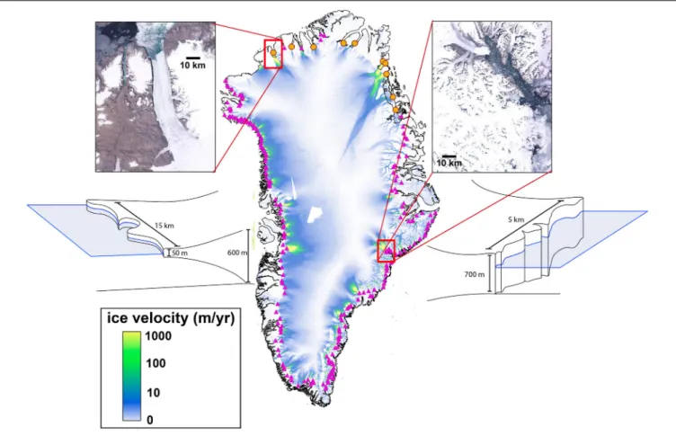
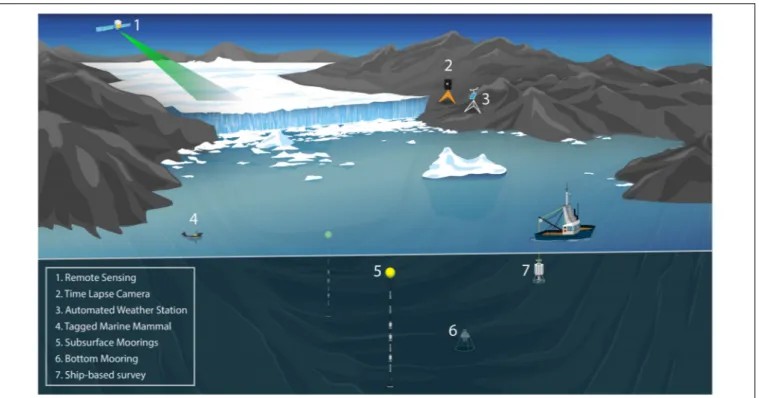
FIGURE 1 |The exchange of heat and freshwater between the ocean and the Greenland Ice Sheet occurs at the margins of over 200 marine terminating glaciers, visible as narrow areas of increased ice flow, distributed around the perimeter of Greenland that discharge into narrow, long and deep fjords. Several of these glaciers are characterized by long (>5 km) floating ice tongues (left inserts, orange circles) but most glaciers have lost their long floating regions (right inserts, pink triangles).
Glaciers identified as having long floating ice tongues greater than 5 km in length, are determined through their height above floatation. Height above flotation is calculated using surface elevation data from the GIMP DEM (Howat et al., 2017) and ice bottom from BedMachine 3 (Morlighem et al., 2017). The background ice velocity is from a 2015–2016 mosaic (Joughin et al., 2017); glacier locations are fromRignot and Mouginot (2012).
(e.g., silica, iron, phosphorus) are exported into the global ocean (Figure 1). These glacial fjords are typically∼100 km long and 5–10 km wide. Outlet glaciers in Greenland are often grounded in hundreds of meters of water. Only a handful of fjords in Northern Greenland have a floating ice tongue (Figure 1, left insets) that covers much of the fjord’s extent (Wilson et al., 2017).
Fjord topography, including the presence of a sill, regulates the exchange of water masses with the continental shelf, where both waters of Atlantic and Arctic origin coexist (Gladish et al., 2015;
Carroll et al., 2017). Fjords with sills deeper than ∼100 m are characterized by a warm, Atlantic-sourced layer underneath a colder, fresher surface layer (Murray et al., 2010;Straneo et al., 2012;Inall et al., 2014;Mortensen et al., 2014).
Key processes that govern the exchanges of heat, freshwater, and nutrients at the ice/ocean boundary, and the upwelling of deep nutrient-rich ocean waters at the glaciers’ margins, include localized plume upwelling driven by the subglacial discharge of ice sheet surface melt at glacier grounding lines (Jenkins, 2011;
Xu et al., 2012;Sciascia et al., 2013;Kimura et al., 2014;Carroll et al., 2015;Cowton et al., 2015;Slater et al., 2015) and distributed melting along the glacier face (Figure 2). The circulation of
waters in the fjord is thought to be regulated by a combination of buoyancy (Motyka et al., 2003), shelf-driven (Jackson et al., 2014; Fraser and Inall, 2018), and wind-driven forcings (e.g., Moffat, 2014; Spall et al., 2017). This circulation guarantees a continuous supply of heat to melt ice (see review by Straneo and Cenedese, 2015) and regulates the export of the strongly diluted meltwater (Beaird et al., 2015, 2017;Jackson and Straneo, 2016). Icebergs, commonly found next to calving glaciers, release meltwater throughout much of the fjord water column as they melt (Enderlin et al., 2014;Moon et al., 2017).
Subglacial discharge, i.e., ice sheet surface melt routed to the ice sheet base via the englacial drainage system (Noël et al., 2016;Van den Broeke et al., 2016; Langen et al., 2017;Wilton et al., 2017), has emerged as a major player in ice sheet-ocean interactions, since it amplifies ice sheet-ocean exchanges (e.g., Jenkins, 2011; Slater et al., 2015). Calving of icebergs, which balances most of the ice flux across the grounding line, is a poorly understood process that is likely influenced by climatic conditions and is a key regulator of glacier dynamics (Schoof et al., 2017). Efforts to extend the temporal record of ice sheet mass loss is the subject of considerable research (e.g., the
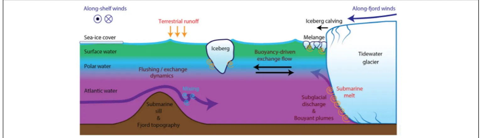
FIGURE 2 |Schematic of a Greenland glacier/fjord system showing relevant physical processes that govern circulation in the fjord and at the glacier-fjord boundary, typical stratification and water masses, and sources of freshwater to the fjord.
ongoing East GRIP Ice-Core Project focusing on the Northeast Greenland Ice Stream).
Building a Case for GrIOOS: The Last Decade
The rapid increase in mass loss from the GrIS began in the early 2000s (Krabill et al., 2004;Rignot et al., 2008;Murray et al., 2015;
Catania et al., 2018;Wood et al., 2018) and it was only a decade later that the importance of processes at the ice sheet-ocean margins became apparent, making ice sheet-ocean interactions in Greenland and globally a novel and rapidly growing area of research. Key to community progress have been a series of workshops, and related follow-up documents, that sought for the first time to bring together the diverse disciplines needed to advance the science.
The first of these workshops, a multi-disciplinary International Workshop on “Understanding the Response of Greenland’s Marine-Terminating Glaciers to Oceanic and Atmospheric Forcing,” was organized by the US Climate and Ocean Variability, Predictability, and Change (US CLIVAR) Working Group on Greenland Ice Sheet-Ocean interactions in June 2013. It brought together over 100 international scientists and program managers with the goals to summarize the current state of knowledge and questions (Straneo et al., 2013) and to develop several key recommendations to make progress (Heimbach et al., 2014). One major recommendation was the collection of long-term time series (both in situand remotely sensed) of critical glaciological, oceanographic, and atmospheric variables at key locations in and around Greenland through the establishment of GrIOOS. The research community recognized that such measurements are needed to provide information on the time-evolving relationships between climate forcing, ice sheet dynamics, and ocean characteristics. The lack of such data has hindered our ability to explain and model the complex interactions among ice-ocean-climate, leaving major gaps in our ability to project future changes. The community noted that GrIOOS data would be critical, not only to validate hypotheses, but also to provide boundary conditions, forcings, and a point of comparison for both ocean and ice sheet model simulations.
Following the recommendations made in the 2014 report, the Study of Environmental Arctic Change Land Ice Action Team, in collaboration with the Greenland Ice Sheet Ocean Interaction Science Network (GRISO), and the Climate and Cryosphere Project (CliC) of the World Climate Research Program, organized a workshop to make progress on the design and implementation of GrIOOS. The resulting 2015 workshop was attended by 47 participants from seven countries, including U.S.
agency program managers (National Science Foundation, NSF, and National Aeronautics and Space Administration, NASA) and a representative of the Greenland government. Participant expertise included oceanography, glaciology, climate and ice sheet modeling, marine ecosystems, and paleoclimatology.
Together, this group examined questions such as: (i) What are the essential ice sheet and ocean variables? What measurements and observing systems already exist? (ii) What should be the structure of the GrIOOS system regarding target observing sites and optimal instrumentation? (iii) How could data be collected, quality controlled, and distributed? Tentative answers to these questions are summarized in Straneo et al. (2018) and have informed the GrIOOS system design discussed here.
Societal Benefits From GrIOOS
Our inability to quantify GrIS-ocean exchanges, and their climate forcing, is a major scientific obstacle to understanding causal origins of past variability and to predicting the future of GrIS and its impact on the neighboring ocean regions, including the marine ecosystems. Connecting science across disciplines and countries, which is necessary to address key climate-related questions, has proven challenging because there is no integrating framework for a comprehensive ice sheet and ocean observing system, including needed structures for data management and dissemination, translating observations to usable model data and parameterizations, and overall cyberinfrastructure to support FAIR (Findable, Accessible, Interoperable, Re-usable) data.
The objectives of GrIOOS are to address all of these challenges by determining essential observations (‘Essential Variables’) for the ice sheet-ocean-atmosphere system, establishing guidelines for instrumentation that can be used across institutions and
nations, creating metadata standards, establishing quality control best practices, and developing a user-friendly platform for FAIR data archiving, access and analysis. Fundamentally, these objectives support overarching goals to understand and project Greenland (and Arctic) ice sheet-ocean interactions and their impact on the ocean, including sea level rise. They explicitly contribute to two of the grand challenges issued to the international scientific community by the World Climate Research Programme and its subsidiaries, such as CLIVAR and CliC: (1) Melting ice and global consequences; (2) Regional sea-level change and coastal impacts.
GrIOOS will also serve other critical societal needs.
Greenlandic communities rely on information about fjords, icebergs, and sea ice conditions for hunting and travel. Most of this information is based on personal experience and shared by word of mouth or social media. For coastal navigation and shipping, the ice service at the Danish Meteorological Institute (DMI) has a long history of mapping sea ice and icebergs hazards, especially around southern Greenland, for navigation purposes.
The ice service is now automated and generates bi-weekly maps, taking advantage of Sentinel satellite imagery to give an overview of sea ice extent and iceberg distribution. With a GrIOOS program in place, we can create improved products that provide higher spatial resolution and, depending on the observation type, better temporal resolution. Such a program can also provide datasets that are requested by local hunters, fishers, policy makers, and business owners. Through coordination with colleagues at Asiaq Greenland Survey, this new or improved data can be shared with local communities in an easily usable, near-real time format, such as through an established GrIOOS data portal, or through appropriate media available to these communities. Asiaq also maintains an interactive Geographical Information System (GIS) website that is heavily used by the local community1, which could provide an additional platform for data integration and access. The Government of Greenland has prioritized “strengthening the population’s knowledge of climate change” and “disseminating information about climate change”
as two of its four main research goals (GCRC, 2015). GrIOOS observations and cyberinfrastructure can support these goals.
International collaboration is also essential for regional engagement in the integration of science and traditional knowledge in ice sheet-marine coupling research. The Pikialasorsuaq partnership is a new collaboration between Greenland, Denmark, and Canada. The Pikialasorsuaq is the Inuit name for the North Open Water Polynya. This polynya is particularly important as a shared resource between Canada and Greenland, affecting biogeochemical processes at the northern limit of Baffin Bay (Barber and Massom, 2007).
The governments of Canada, Greenland, and Denmark are currently discussing how to manage the Pikialasorsuaq region as an international shared resource. Based on the concept of a larger Baffin Bay Observing System (Rysgaard and BBOS Committee, 2017), the GrIOOS system will include an effort to bring traditional knowledge from communities surrounding the
1www.nunagis.gl
North Open Water polynya into the ice sheet-ocean observing system framework.
VISION FOR A GREENLAND ICE SHEET-OCEAN OBSERVING SYSTEM
The overarching vision for GrIOOS is the simultaneous observation of glaciological, oceanic, and atmospheric ‘essential variables’ (bothin situand remotely sensed) at ice sheet-ocean sites around Greenland, to be sustained over the coming decades.
The observation should be sustained over multiple cycles of dominant atmospheric and oceanic modes of variability (e.g., National Academies of Sciences et al., 2016), in particular the North Atlantic Oscillation, Greenland Blocking, Atlantic Multidecadal Variability, and Pacific Decadal Variability. It should also cover the era of continuous satellite observations of several essential variables, which will be integrated with thein situ GrIOOS system and data.
The ensemble of GrIOOS sites should cover a range of ice sheet-ocean configurations, connect to all major oceanic basins around Greenland, be representative of the different climatic regimes, and capture systems thought to be dominant contributors to GrIS mass loss. The minimum set of essential variables to be collected at each site is motivated by present-day understanding of the key oceanic, glaciological, and atmospheric variables behind the processes that govern ice sheet-ocean exchanges of heat, freshwater, and nutrients. Additional inputs for any GrIOOS site are bathymetry and bed elevation. We refer to these as foundational datasets, which are critical but only need to be collected once. Ancillary measurements at a site, such as sediment cores that provide context for GrIOOS observations to be extended back in time, e.g., via paleo-proxy reconstructions (e.g.,Andresen et al., 2012;Henry et al., 2016), or seismic and geodetic stations that connect GrIOOS to other scientific communities, are also highly desirable (e.g.,Nettles and Ekström, 2010;Bevis et al., 2012).
The development and maintenance of GrIOOS will require close international collaboration. GrIOOS implementation will need to be coordinated amongst different countries, paying close attention to minimizing costs and optimizing shared logistics.
Data processing protocols and data sharing practices must be identified, shared, and maintained. Quick, open, and centralized access to data is vital. Below we explain in detail the proposed GrIOOS framework.
In developing GrIOOS, we seek to follow the Framework for Ocean Observing (Task Team for an Integrated Framework for Sustained Ocean Observing, 2012) in an extended form that captures both the fundamentally multi-disciplinary nature of the ice sheet-ocean system, and the detail required to advance process level understanding.
Identifying the Essential Variables of a GrIOOS Site
Several key constraints are taken into consideration in identifying the ensemble of essential variables gathered at each GrIOOS site.
First the ensemble of these variables should be sufficient input
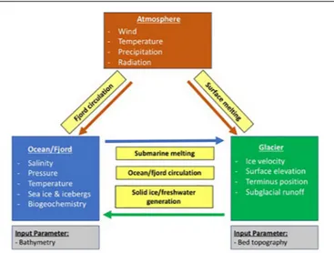
FIGURE 3 |Identified essential variables and their interconnection (inside boxes) at a GrIOOS site.
to algorithms or models that describe variations in the ice sheet- ocean processes that are relevant to addressing the questions identified above (Figure 3). Second, the essential variables should be practical to obtain, i.e., measurable and sustainable in terms of cost or derivation. Third, these variables should be relatively easy to relate to the larger scale oceanic, glaciological, and atmospheric context. Here, we summarize the relevant processes within the three focus areas identified above and identify essential variables that can represent their variability.
Sea Level Rise
Future sea level rise from the GrIS depends on mass loss through surface melt and through solid ice discharge of icebergs at the ice sheet-ocean boundary. Improving understanding of ice sheet- ocean interactions will inform research on the location and magnitude of ice sheet variability due to atmospheric and oceanic changes. To examine the ice sheet-ocean-atmosphere system, we have identified: ice sheet surface velocity; ice sheet surface elevation (and ice thickness via bed topography data); terminus position; surface runoff and subglacial discharge as the minimum set of essential variables (Table 1).
Ice sheet surface velocity, combined with ice thickness and grounding line information, can be used to calculate ice flux at marine termini around Greenland (e.g., Rignot et al., 2011;
Enderlin et al., 2014). Time-series of these variables are also essential in unraveling the processes governing flow variability (e.g., Stearns and van der Veen, 2018). Acceleration, thinning, and retreat often occur near-coincidentally, driven by processes at the ice-bed and ice-ocean interface that are impossible to observe directly.
Frontal ablation at the ice-ocean interface, which includes submarine melting and iceberg calving, all influence ice sheet behavior and ice loss (Straneo et al., 2013; Kjeldsen et al., 2017). Submarine melting is largely thought to be controlled by the thermal forcing of the ocean waters reaching the glacier (Figure 2), and is amplified by large ocean velocities,
such as those due to subglacial discharge driven turbulent, upwelling plumes at the glaciers’ margins during the melt season (Mortensen et al., 2013; Bendtsen et al., 2015; Mankoff et al., 2016; Jackson et al., 2017). Calving is accelerated in regions undercut via submarine melting (described above;Bartholomaus et al., 2013; Chauché et al., 2014; Fried et al., 2015), but can also occur when the terminus reaches flotation and basal crevasse propagation leads to full-thickness calving (James et al., 2014; Murray et al., 2015). Essential observations needed to constrain submarine melting: are subglacial discharge, and ocean temperature and salinity as a function of pressure (Table 1), The essential observations of terminus position and ice velocity, combined with calculations of submarine melt will inform research on calving processes, ice sheet response to ocean change, and, ultimately, sea level rise.
Freshwater Export
Glaciers release freshwater at the ice sheet-ocean margins as solid ice (icebergs) and meltwater. Meltwater enters the fjords as surface runoff, submarine melt across the termini, or subglacial discharge (Figure 2). Icebergs undergo considerable melting as they transit through the fjords, giving rise to an additional meltwater flux (distributed along the iceberg depth) and a residual iceberg export at the fjord’s mouth. This melting, in turn, is largely controlled by the fjord circulation and temperature structure. The export is controlled by local winds, the fjord circulation and fjord bathymetry.
Meltwater released at depth along the glacier face (submarine melt and subglacial discharge) creates plumes that rise, entrain large volumes of deep fjord waters, and produce a much greater transport than the volume of meltwater released (e.g., Motyka et al., 2003;Beaird et al., 2018). While the details of the processes controlling the dilution and export of the meltwater and of icebergs, from the glacier and fjord, are complex, they are thought to be largely controlled by: (1) the release of subglacial discharge and surface runoff; (2) the iceberg flux; (3) the temperature of the fjord waters; (4) the fjord circulation; (5) local winds. These in turn, can be described in terms of the surface mass balance components, the calving flux, properties inside the fjord and on the nearby shelf (since this gradient controls the fjord/shelf exchange), local and regional winds. Note that while it would be highly desirable to include fjord velocities (or circulation) as an essential variable, these measurements are costly and largely uncertain due to the high spatial and temporal variability of velocities in these narrow fjords (Mortensen et al., 2014;Jackson and Straneo, 2016;Boone et al., 2017). Information about iceberg distribution and sea ice coverage is also critical for classifying ice hazards, which is a crucial metric for shipping, industrial development, and local community activities in the marine areas surrounding Greenland (e.g.,Barber et al., 2014).
Impact on Biogeochemistry and Ecosystems
The timing, mode of delivery, properties, and magnitude of freshwater export into the ocean fundamentally shape ocean biogeochemistry. Plumes of meltwater and entrained ocean waters rising at the glacial margin drive a vertical transport of dissolved nutrients and sediments toward the surface
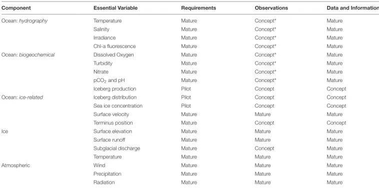
TABLE 1 |GrIOOS essential variables, with information about readiness levels for component requirements, observation instruments and methods, and data and information systems.
Component Essential Variable Requirements Observations Data and Information
Ocean:hydrography Temperature Mature Concept∗ Mature
Salinity Mature Concept∗ Mature
Irradiance Mature Concept∗ Mature
Chl-a fluorescence Mature Concept∗ Mature
Ocean:biogeochemical Dissolved Oxygen Mature Concept∗ Mature
Turbidity Mature Concept∗ Mature
Nitrate Mature Concept∗ Mature
pCO2and pH Mature Concept∗ Mature
Iceberg production Pilot Concept Concept
Ocean:ice-related Iceberg distribution Pilot Concept Concept
Sea ice concentration Pilot Concept Concept
Surface velocity Mature Mature Mature
Terminus position Mature Concept Concept
Ice Surface elevation Mature Mature Mature
Surface runoff Mature Mature Mature
Subglacial discharge Mature Concept Mature
Temperature Mature Mature Mature
Atmospheric Wind Mature Mature Mature
Precipitation Mature Mature Mature
Radiation Mature Mature Mature
The readiness levels, moving from concept to pilot to mature, are based on terminology for the Framework for Ocean Observing (seeFigure 8inTask Team for an Integrated Framework for Sustained Ocean Observing, 2012), with different requirements for each category: requirements, observations, and data and information.
∗Locational challenges add to ‘concept’ classification.
ocean, where they can impact the growth of phytoplankton by respectively fueling primary production or altering light penetration and optical properties. Measurements of nitrate, a primary limiting nutrient present in low concentration in meltwater but abundant in the deep ocean, alongside turbidity, in this way serve as essential tracers for ice- ocean exchanges and glacier-driven circulation, as well as nutrient availability. The response of phytoplankton to glacial modification of upper water column physical and chemical properties can in turn be examined through measurement of chlorophyll-a fluorescence and dissolved oxygen. Alongside measurements of ambient light, these parameters can, in concert, give insight into primary productivity rates and the biomass of organic carbon available to higher trophic levels, important ecosystem properties. The integrated response of the carbon cycle to ice-ocean exchanges, including the overall magnitude and sign of the atmosphere-ocean carbon flux, is a function of both biological cycling and thermodynamic effects stemming from physical mixing of glacial and ocean water masses (Meire et al., 2015). Time series of pCO2 and pH, alongside biological parameters previously described, are therefore essential variables to constrain carbon cycle response (Figure 3).
The Relevant Essential Variables
Based on a summary of the processes and major controlling variables outlined above, and in consideration of both feasibility and reliability of existing technologies for long- term measurement, we suggest the following essential oceanic,
glaciological, and atmospheric variables for each GrIOOS site (Table 1):
• Oceanic variables include temperature and salinity as a function of pressure both within the fjord and across the nearby shelf. Sea ice cover, iceberg production, and iceberg distribution are also essential. Biogeochemical variables needed to characterized productivity include downwelling irradiance, chlorophyll-a fluorescence, and dissolved oxygen. Turbidity and nitrate are needed to quantify seasonality in nutrient availability associated with glacial discharge and fjord circulation. Finally, pCO2 and pH are needed to constrain the carbon cycle response.
Tracking of properties both inside the fjord and on the nearby shelf is needed to separate remote and local drivers of variability.
• Glaciological variables include ice velocity, surface elevation, ice thickness (via bed and surface elevation), terminus position, surface melt (i.e., that generates surface runoff) and subglacial discharge. These variables will allow us to calculate iceberg calving rates, ice volume changes, and freshwater discharge at the GrIS marine margin.
• Atmospheric variables include local weather data (winds, air temperature, precipitation, radiation, etc.) to provide information essential to estimating the regional and fjord- scale atmospheric forcing of the ice sheet and ocean surface.
• Additional foundational datasets critical for any GrIOOS site are bedrock and ocean bathymetry.
FIGURE 4 |Example of potential instrumentation for a GrIOOS site located at the margins of a tidewater glacier (note: not to scale).
How to Get the Essential Variables for Each GrIOOS Site
It is envisioned that the essential variables described above (and in Table 1) will be gathered at each site either as in situ measurements or as derived quantities from, for example, remote sensing. A generic GrIOOS site is depicted in Figure 4. For all essential variables, there is a strong need for year-round observations. High temporal resolution (as often as hourly to weekly depending on variable) measurements are required since it is unclear which timescales govern both the oceanic forcing and the glacier response, or whether threshold behavior exists that only bears out during certain environmental conditions.
Engagement with communities located near GrIOOS sites will be a key part to the temporal sampling required.
Ocean
Ocean essential variables require year-round measurements both in the glacier vicinity (typically in the fjord) and on the nearby continental shelf. Depending on the fjord/glacier type, the way these measurements are achieved may differ substantially.
Floating ice shelves (or ‘floating tongues’) offer the possibility of suspending instruments from the ice through bore holes that are expensive to drill but provide ideal platforms. Tidewater glaciers with substantial calving are challenging because of the deep draft icebergs and general inaccessibility of the region.
These require site specific strategies that may include subsurface moorings (Figure 4). Sensors deployed on marine mammals may be appropriate for some sites where other technologies are deemed impractical. Biogeochemical sensors present additional challenges that will also necessitate site-specific strategies.
A subset of biogeochemical sensors (e.g., fluorescence, O2, pCO2, pH) need to be deployed in the upper 10–50 m of the water column where major biological processes and freshwater export take place. By contrast, sensors used to characterize links between physical processes and chemical properties of the ocean (e.g., nutrient fluxes and distributions) may in certain cases be deployed subsurface.
The size and distribution of icebergs in fjords and the surrounding ocean are important to characterize for their impact on freshwater- and nutrients dynamics. New efforts to quantify iceberg distributions are now possible given the robust temporal coverage of both optical and radar satellite imagery over the Arctic. Ocean nodes should integrate remote sensing results of both iceberg distribution and sea ice coverage, which are essential for freshwater flux calculations (Moon et al., 2017;
Sulak et al., 2017). Iceberg detection from Sentinel satellites around Greenland has been automated by the DMI and daily plots for several distinct locations are displayed on the Danish public outreach website polarportal.dk, based on the methods of Buus-Hinkler et al. (2014) but at finer spatial resolution of 40 and 10 m. While this technique is able to distinguish icebergs at unprecedented resolution, it shares, with other remote sensing data products, the disadvantages of limited temporal and spatial coverage and is not capable of distinguish icebergs trapped within sea ice or mélange in front of calving outlet glaciers. Finally, it is notable that despite the large fraction of discharge from the GrIS occurring as solid ice, little information is available concerning how icebergs affect nutrient cycling within Greenland’s fjords, making iceberg observations also critical for ocean biogeochemistry.
Glacier
Most glacier essential variables (ice surface velocity, terminus position, ice sheet surface elevation) can be acquired via remote sensing sensors already in orbit and mature analysis techniques. Some variables can already be acquired from consistently archived and served data streams and will not require significant GrIOOS investment. For example, both optical and radar satellites now allow weekly to monthly measurements of ice surface velocity, which is systematically processed and served through U.S. and European data archives. Some datasets, however, require further GrIOOS science and research development. In particular, terminus position is not currently provided in a systematic way, largely consisting of sporadic terminus shapefiles available from individual investigators.
Existing networks and data sets to support development of glacier and ice sheet essential variables are discussed in Section “Glacier and Ice Sheet.” Additional in situ observations of the outlet glacier system could also take advantage of ocean deployments for additional sensors to improve understanding with satellite-based observations and time-lapse cameras to provide high temporal and spatial information (Figure 4). The best current source for surface mass balance information are regional climate models (see Dynamical and Statistical Reconstructions). We envision essential variables will be linked on a website that would bring together the disparate data sets for the general purpose of quantifying the spatio-temporal variability in glacier behavior (see Data Protocol and Management).
Atmosphere
The atmosphere node provides variables that support both glacier and fjord measurements. At the local scale measurements are obtained via Automated Weather Stations (AWS; Figure 4).
AWS deployed at locations adjacent to the glacier terminus can provide essential variables (air temperature, winds, precipitation, radiation) and other standard meteorological observations (Table 1). These data can also improve remote sensing and reanalysis products. Depending on the location, such measurements may be available through several of the existing meteorological station networks, e.g., DMI, see Weather Station Data). At the regional scale, estimates of air temperature, winds, pressure, and other meteorological parameters are available through regional climate model or global atmospheric analysis, forecast or reanalysis products (see Dynamical and Statistical Reconstructions). These data will fulfill many of the variable needs for capturing regional-scale atmospheric conditions over the glacier-fjord-continental shelf system. In addition, large-scale circulation indices, such as the Greenland Blocking Index (Hanna et al., 2016, 2018), will be helpful for contextualizing ice sheet- atmosphere-ocean interactions.
Foundational Datasets: Bathymetry and Bed Elevation
Ice sheet bedrock topography and fjord bathymetry are critical foundational datasets. Significant efforts have been made over the last decade to improve estimates of ice sheet bed elevation, particularly beneath the outlet glaciers of the GrIS, with airborne ice-penetrating radar (Leuschen et al., 2018). In addition, new
bathymetric and airborne gravity surveys within multiple glacier fjords in Greenland have been made over the last few years as interest in ice sheet-ocean interactions has increased (e.g.,Fenty et al., 2016; Rignot et al., 2016; Kjeldsen et al., 2017; Millan et al., 2018). These provide an even more detailed picture of the topography beneath glacier termini and within the fjord.
Together, these types of observations have been used to construct a seamless bed elevation product across the GrIS ice sheet-ocean margin using a mass-conservation approach that provides a best estimate for the bed topography constrained by observational data (Morlighem et al., 2011, 2017). Since these new data use both ice-penetrating radar and bathymetric data, grounding line depth estimates have improved dramatically over previous estimates and provide a more accurate picture of the geometric setting for critical outlet glaciers terminus regions. Even with these improvements, many outlet glaciers (adjacent) within the GrIS have not been surveyed with ice penetrating radar (bathymetric mapping) and are poorly constrained in the mass-conservation inversion. Any additional bedrock/bathymetric data collected as part of GrIOOS should therefore be readily made available to improve the existing database.
Characteristics of GrIOOS Sites
The ensemble of GrIOOS sites should span a range of geometries that take into account the glacier/fjord depths, fjords with and without sills, glaciers with and without floating termini, and different oceanic basins. Choice of the sites should take into account existing measurements, noting sites that are already being monitored that could become GrIOOS sites with minimum additional measurements. Proximity of other observing networks (see below) to sites can optimize sustainability, provide broader context, and allow shared logistics costs. Sites close to inhabited or regularly serviced centers allows for accessibility at reduced costs and may be a source of information to the local community.
There should be a focus on the largest contributors to Greenland Ice Sheet mass loss, and the proximity of paleo records should also be taken into account.
At the initial GrIOOS development meeting, several possible observational sites were suggested based on voting of each participants’ top three sites and the considerations described above, such as existence of ongoing observations, logistical support, scientific rationale, and societal rationale.
The glacier/fjord sites with the most votes were Helheim Glacier/Sermilik Fjord, 79 N/NE Greenland Ice Stream (NEGIS), and Jakobshavn Isbrae/Ilullisat Icefjord, with additional priority sites listed here in order of voting (Table 2). The top three sites are dominated by glaciers that calve via full-thickness events and where melt-induced terminus change may play a reduced role (Fried et al., 2018). In a fully implemented GrIOOS, care should be taken to include a broad range of glacier settings, defined by the glacier dynamic behavior, and fjord settings, defined by geometry and proximity to distinct open ocean regions.
Additionally, during the previous GrIOOS workshop, participants helped to identify and discuss lessons learned from other ongoing observational programs, such as the Geological Survey of Denmark and Greenland (GEUS) Program for Monitoring of the Greenland Ice Sheet (PROMICE), or
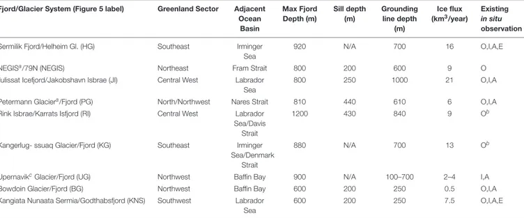
TABLE 2 |Characteristics of potential GrIOOS glacier-fjord sites, including the ocean basin adjacent to link to existing open ocean measurements, the fjord and glacier geometry to ensure a diversity of glacier/fjord types, Greenland sector, and whetherin situmeasurements of ocean (O), ice (I), atmosphere (A), and ecosystem (E) variables exist now or in the past.
Fjord/Glacier System (Figure 5 label) Greenland Sector Adjacent Ocean
Basin
Max Fjord Depth (m)
Sill depth (m)
Grounding line depth
(m)
Ice flux (km3/year)
Existing in situ observation
Sermilik Fjord/Helheim Gl. (HG) Southeast Irminger
Sea
920 N/A 700 16 O,I,A,E
NEGISa/79N (NEGIS) Northeast Fram Strait 800 200 600 9 O
Ilulissat Icefjord/Jakobshavn Isbrae (JI) Central West Labrador Sea
800 250 1000 21 O,I,A
Petermann Glaciera/Fjord (PG) North/Northwest Nares Strait 810 440 610 6 O,I,A
Rink Isbrae/Karrats Isfjord (RI) Central West Labrador Sea/Davis
Strait
1200 430 840 9 Ob
Kangerlug- ssuaq Glacier/Fjord (KG) Southeast Irminger Sea/Denmark
Strait
880 N/A 700 13 Ob
UpernavikcGlacier/Fjord (UG) Northwest Baffin Bay 900 N/A 100–700 2–4 I,A
Bowdoin Glacier/Fjord (BG) Northwest Baffin Bay 600 200 250 0.5 O,I,A
Kangiata Nunaata Sermia/Godthabsfjord (KNS) Southwest Labrador Sea
600 200 250 7.5 O,I,A,E
The listed order represents the number of votes obtained for developing each glacier/fjord system as a GrIOOS site (see text).aThe Northeast Greenland Ice Stream/79 N and Petermann Glacier both terminate in perennial floating ice tongues.bTime-series of ocean variables exist here, but only for limited time ranges in the past and not at present.cRanges are given since four glaciers flow into Upernavik Fjord (Ahlstrøm et al., 2013).
through the Global Ocean Observing System Framework for Ocean Observing (Task Team for an Integrated Framework for Sustained Ocean Observing, 2012). Several potential key requirements were identified:
• Light and sustainable: Logistically or instrumentally expensive observing systems are difficult to maintain over time. Simple logistics, and ones that would make use of interested communities, are best. However, previous efforts [e.g., US Geological Survey (USGS) monitoring for mountain glaciers] have shown that it is best to aim for oversampling during the first several years of the observing system, with the objective to identify key sites for sustained observations, accommodating potential needs to scale down the observing system over time.
• Monitoring requires proven technology: Although testing new technology is an interesting prospect if it can reduce later costs, an observing system is not the best place to implement new technologies.
• Build on available logistics and programs: Although programs that are already running would not easily scale up, they can provide logistical support for additional instrumentation deployment, if necessary.
EXISTING NETWORKS
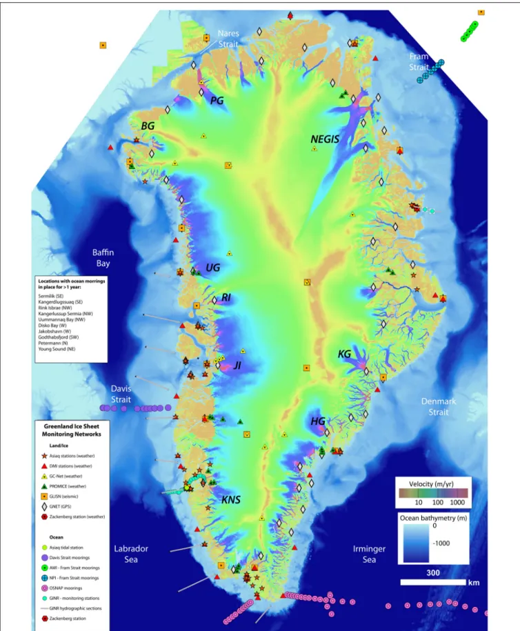
Interest in the GrIS and surrounding fjords and ocean has grown rapidly over the last few decades and led to an expansion of monitoring networks both in situ and from remote sensing observations (Figure 5). GrIOOS will be developed to connect with and leverage these existing networks. In particular, the
connection with regional programs will provide the needed ‘far- field’ connection of GrIOOS’ sites to the ocean (continental shelf and large scale ocean); the ice sheet and the atmosphere. Here, we outline a number of these existing research and observation activities (seeFigure 5for location).
Ocean
Moored Arrays
The mooring array in Fram Strait (de Steur et al., 2014) to measure Arctic Outflow was deployed in 1997 as a government funded monitoring system collaboration between Norwegian Polar Institute (Norway) and the Alfred Wegener Institute (Germany). The array records temperature, salinity, currents, ice thickness and ice drift, and is complemented by annual conductivity/temperature/depth (CTD), lowered acoustic Doppler current profiler (LADCP) and tracer transects in August and September (Figure 5). It is expected that it will be maintained for at least another decade. The array is concentrated in deeper water and lacks moorings on the Greenlandic continental shelf (due to ice hazards), however, repeat CTD transects are conducted on the shelf whenever possible.
A mooring array across Davis Strait was deployed in 2004 as a US-Canadian collaborative project to measure Arctic outflow west of Greenland (Curry et al., 2014).
The mooring array spans across the continental shelves (Figure 5) and measures velocity, temperature, salinity, sea ice thickness. It is supplemented by marine mammal acoustics, year-round glider observations, and annual or biennial hydrographic sections. Hydrographic measurements also include macro-nutrient concentrations (i.e., nitrite plus nitrate, silicate, phosphate, ammonium) and oxygen
FIGURE 5 |Map of primary existingin situnetworks and long-term measurements around Greenland, overlaid on a map of ice velocity (Joughin et al., 2011) and bathymetry (Morlighem et al., 2017). Glaciers listed inTable 2are identified using labels fromTable 2.
isotopes (δ18O). The future of the network is uncertain and dependent on funding.
Overturning in the Subpolar North Atlantic Program2 is an international trans-basin observing system to measure the meridional overturning circulation through mooring arrays (Figure 5), repeat hydrographic transects, and glider deployments (Lozier et al., 2017). The observing network, which includes two mooring arrays on the southeast and southwest Greenland shelves and slopes, was installed in 2014 and currently funded through 2020. It is expected that it will be maintained for a decade.
Hydrographic Surveys
The Greenlandic fisheries industry has records, dating back to 1990, of bottom temperature collected during bottom trawler shrimp density surveys off the southwest coast (e.g., Holland et al., 2008). Approximately 50% of the stations are reoccupied annually. The Icelandic mackerel survey on the east coast has hydrographic measurements starting from 2013 that extend from Greenland to Iceland and Norway.
Hydrographic transects in Godthåbsfjord have been conducted since 2007 by the Greenland Institute of Natural Resources (GINR) and include measurement of physical, biological, and chemical variables (Figure 5). Ice-free conditions in the fjord mean this survey is conducted year-round from small vessels. One station near Nuuk is monitored monthly, where a suite of ecosystem sampling is conducted in concert with the hydrographic observations. Ecosystem monitoring is being carried out only at a few other sites around Greenland, but resources are limited and marine ecosystem observations only begin in 2002. Moorings have been maintained during the last decade at several locations.
Hydrographic transects in West Greenland: GINR also monitors across the continental shelf of west Greenland during yearly surveys (Figure 5) in June and July3; previously these surveys were handled by DMI on behalf of the Greenland Institute of Natural Resources (e.g., Myers et al., 2009).
Additionally CTD measurements are collected inshore during yearly fishery surveys in Maniitsoq, Disko Bay, Uummannaq, and Upernavik.
The Oceans Melting Greenland project is a 5-year NASA program that began in 2015 to observe water temperatures around the coast of Greenland (Figure 5) and measure how marine terminating glaciers react to the presence of Atlantic Water (Fenty et al., 2016). The project consists of annual aerial ice topography measurements and gravimetry of glacier margins and the deployment of 250 Airborne expendable CTD probes (AXCTDs) to measure the properties and extent of Atlantic Water around the coast.
The GEOTRACES project is an ongoing, coordinated international activity to quantify the supply, removal, and distribution of bioessential micronutrients (such as iron) in the ocean. The completed cruise sections GA01 (North Atlantic/Labrador Sea), GN02 (Labrador Sea/Baffin Bay) and
2www.o-snap.org
3https://archive.nafo.int/open/sc/2015/scr15-001.pdf
GN05 (Fram Strait) provide an invaluable dataset to measure trace chemical species in the ocean around Greenland. The GN05 section was notable for proceeding to sample within close proximity to the 79N glacier and the GA01 section includes shallow shelf stations which show a terrestrial influence on shelf water properties. Whilst the GEOTRACES program has an intentional offshore focus, there is now a clear possibility of process studies to bridge the gap between these extensive offshore sections and fjord/shelf regions to understand how far offshore meltwater and glacially derived particles influence the biogeochemical cycling of essential micro-nutrients in the ocean.
The Labrador Sea Monitoring Program of Fisheries and Oceans Canada has collected physical, chemical, and biological observations along a hydrographic transect across the Labrador Sea (corresponding to Atlantic Repeat Hydrography Line 7 West of the World Ocean Circulation Experiment) since 1990.
Measurements span Hamilton Bank on the Labrador Shelf to Cape Desolation on the Greenland Shelf. The transect is occupied annually, although frequency is dependent on funding (Yashayaev and Loder, 2017).
Autonomous Sampling
Large scale ocean properties can be obtained from the Argo float program that, since 2006, maintains a global array of more than 3000 free-drifting profiling floats that measure hydrographic properties in the upper 2000 m of the ocean (Roemmich et al., 2009). This program is complemented by the Biogeochemical-Argo float program (Claustre et al., 2010;
Gruber et al., 2010), which alongside physical parameters collects biogeochemical measurements. These floats are not useful on the Greenland continental shelf but do provide boundary conditions to monitor long-term average ocean basin property changes around Greenland.
Water property information is also obtained by tagging marine mammals, and a central repository for these data already exist in the international Marine Mammals Exploring the Ocean Pole to Pole program (Treasure et al., 2017).
These temperature/salinity profiles provide useful data on the continental shelves (e.g., Sutherland et al., 2013) or offshore (Laidre et al., 2010; Grist et al., 2014), and are potentially a way forward for collecting more in situ data inside fjords (e.g., Mernild et al., 2015) as well as a connection to the ecosystem response of higher-trophic level animals influenced by Greenland’s glacial fjords (Laidre et al., 2016).
Remote Sensing
Remote sensing data products can provide important oceanographic information (such as sea surface salinity and temperature), but are not currently generated at the scale that is useful for GrIOOS. A few of these products are potentially useful for fjord-scale processes, such as subglacial outlet plumes, sea-ice cover, iceberg drift and biological productivity (ocean color). However, satellites are limited in their ability to observe subsurface features (e.g., phytoplankton blooms, glacial and sediment plumes) that are relevant to GrIOOS science goals. Sea surface height can be measured via satellite altimetry, but with challenges near the coast and with limited
coverage at high latitudes (Cipollini et al., 2016). Sediment plumes can be monitored by MODIS Aqua/Terra and Landsat 8, and ocean color measurements (characterizing biomass of primary producers and productivity) are collected by SeaWiFS, MODIS, and Sentinel 3-A, among others. Most of these variables, however, are considered ancillary to the essential ocean variables for GrIOOS.
Remote sensing of sea ice can include active and passive microwave estimates of the thermodynamic state of fast-ice fringes of sea ice, sea ice drift estimates (including export pathways on the west and east sides of Greenland), presence of significant freshwater sea ice, sea ice dynamic properties through coupling to glacier solid and liquid phase fluxes, and estimates of the optical properties of the sea ice through microwave-optical radiative transfer techniques (e.g., Barber, 2005). Specifically, both Landsat (optical) and Sentinel (optical, radar) satellite imagery can be used to identify sea ice distributions near the Greenland coast. The combination of Landsat and Sentinel imagery allows for the near-daily classification of features after 2016. Prior to the launch of the Sentinel satellites, repeat observations with Landsat occur every 16–18 days since
∼1999. Note that even medium resolution sea ice concentration products, such as 4-km Multisensor Analyzed Sea Ice Extent data (and, in 2015-2016, 1-km resolution data), fail to provide accurate sea ice concentrations in Greenland fjords. Future GrIOOS efforts would include the systematic production of these data at temporal and spatial scales relevant for fjord dynamics.
Glacier and Ice Sheet
Surface Speed
Both optical and radar remotely sensed data can be used to derive velocity data. Optical data has the benefit of multiple bands of data, which can be useful for co-processing velocity with other information, but imaging the ice surface through clouds or darkness is not possible. Radar data avoid these problems but does not include additional bands of data. Satellite coverage for both optical and radar data has expanded substantially over the last two to three decades, with additional satellite launches for both optical and radar instruments planned within the next few years. Velocity data are now available in weekly to monthly time resolution via projects including GoLIVE (Global Land Ice Velocity from Landsat 8 Extraction4); ITSLIVE (Intermission Time Series of Land Ice Velocity and Elevation), which will begin in 2019; and NASA MEaSUREs5, all with key glaciological data hosted at the National Snow and Ice Data Center. Velocity data are also available for more limited areas via the ENVEO Cryoportal6, CPOM Data Portal7, and Technische Universitat Dresden8. The European Space Agency’s (ESA) climate change initiative for the GrIS has operationally produced a number of relevant remote sensing data products including ice sheet velocity, calving front position, surface elevation change and
4nsidc.org/data/golive
5nsidc.org/data/measures
6cryoportal.enveo.at
7www.cpom.ucl.ac.uk/csopr/iv
8data1.geo.tu-dresden.de/flow_velocity
grounding line position. These datasets are updated semi- annually and are freely available (e.g.,Mottram et al., 2018).
Terminus Position
As a result of recent interest in the various processes influencing glacier termini there has been renewed interest in tracking glacier terminus changes over time (Bjørk et al., 2012). Currently yearly observations of the terminus position are available (Murray et al., 2015;Joughin et al., 2017) for the entire ice sheet, including via NASA and ESA. Regional subsets of glaciers have more frequent observations of terminus position, up to twice-monthly in some regions (e.g.,Seale et al., 2011;Carr et al., 2015;Murray et al., 2015;Catania et al., 2018), but these records are dispersed among individual researchers or archives. GrIOOS will need to build on these existing efforts to establish a consistent and complete terminus position data stream.
Surface Elevation
From 1993 to 2003 surface elevation data have been acquired over the GrIS to understand glacier dynamic evolution in response to climate forcing with NASA’s airborne laser altimeter (Krabill et al., 1999; Abdalati et al., 2002). From 2003 to 2009 NASA’s ICESat mission provided laser altimetry data over the entire ice sheet and altimetry is now being continued through to the recent launch of ICESat-2. In the interim, NASA’s Operation Icebridge has provided continuous elevation data9. Combined, these data are used to constrain modeled estimates of elevation change for the entire ice sheet over the entire duration that observations are available (Csatho et al., 2014). In addition to laser altimetry, surface elevation change observations from additional airborne and satellite missions have enabled the creation of digital elevation models (DEMs) for the GrIS. In some cases these DEMs have been created from historical air photos acquired in stereo to produce elevation data extending back to the late 1970s (Korsgaard et al., 2016). Additional DEMs have been created from the commercial vendor DigitalGlobe through its provision of high-resolution optical imagery of the polar regions over the launch of six WorldView spacecraft (Shean et al., 2016).
DigitalGlobe coverage began in 2009 with sporadic coverage until 2012, with the periphery of the GrIS covered with stereo-pairs every year since. Data are currently processed and made available through the Polar Geospatial Center (Porter et al., 2018). The Polar Geospatial Center also serves time-stamped ArcticDEM strips. A useful summary of the last 25 years of surface elevation change is given bySørensen et al. (2018)based on ESA Greenland data from ERS, ENVISAT and Cryosat-2.
Surface Runoff and Subglacial Discharge
The estimate of ice sheet surface mass budget and runoff, routed through individual glacier catchments, is critical for quantifying the spatio-temporal distribution of meltwater-driven terminus melt as well as freshwater discharge and the timing and magnitude of biogeochemical transports. However, ice sheet SMB and runoff continues to be poorly validated at the outlet glacier scale because of the difficulties involved in measuring
9icebridge.gsfc.nasa.gov