How to apply the complementarity and coupling theorems in MCR methods: Practical implementation and application to the Rhodium-catalyzed hydroformylation.

(1)

How to apply the complementarity and coupling theorems in MCR methods:

Practical implementation and application to the Rhodium-catalyzed hydroformylation.

Mathias Sawallâ, Christoph Kubis^b, Robert Franke^c,d, Dieter Hess^c, Detlef Selent^b, Armin Börner^b, Klaus Neymeyrâ,b

aUniversit¨at Rostock, Institut f¨ur Mathematik, Ulmenstraße 69, 18057 Rostock, Germany

bLeibniz-Institut f¨ur Katalyse e.V. an der Universit¨at Rostock, Albert-Einstein-Straße 29a, 18059 Rostock

cEvonik Industries AG, Paul-Baumann Straße 1, 45772 Marl, Germany

dLehrstuhl f¨ur Theoretische Chemie, Ruhr-Universit¨at Bochum, 44780 Bochum, Germany

Abstract

Multivariate curve resolution techniques can be used in order to extract from spectroscopic data of chemical mixtures the contributions from the pure components, namely their concentration profiles and their spectra. The curve resolution problem is by nature a matrix factorization problem, which suffers from the difficulty that the pure component factors are not unique. In chemometrics the so-called rotational ambiguity paraphrases the existence of numerous, feasible solutions. However, most of these solutions are not chemically meaningful.

The rotational ambiguity can be reduced by adding additional information on the pure factors like known pure component spectra or measured concentration profiles of the components. The complementarity and coupling theory (as developed in J. Chemometrics 27 (2013), 106-116) provides a theoretical basis for exploiting such adscititious information in order to reduce the ambiguity. In this paper the practical application of the complementarity and coupling theory is explained, a user-friendlyMATLABimplementation is presented and the techniques are applied spectral data from the Rhodium-catalyzed hydroformylation process.

Key words: spectral recovery factor analysis complementarity and coupling Rhodium-catalyzed hydroformylation process.

1. Introduction

Consider a chemical reaction system to be given with several (potentially unknown) chemical components. Spectroscopic measurements on this system are assumed to result in a series of k spectra. Each spec- trum is a vector with n absorbance values of the chemi- cal mixture with respect to a fixed wavelength grid. This spectral data can be stored row-wise in a k-times-n ma- trix D.

The matrix formulation of the Lambert-Beer law says that D has a factorization

D

k×n

=C

k×s

A

s×n

, (1)

where the concentration factor C ∈R^k×s is a nonnegative matrix which contains column-wise the concentra- tion profiles of the s pure components with respect to the given time-grid. The spectral factor A ∈R^s×n contains row-wise the pure component spectra. Nonlinearities

and measurement errors can be taken into account by adding a small error matrix E ∈ R^k×nto the right-hand side of (1).

In chemical applications only the spectral data ma- trix D is given and the unknown number s of indepen- dent components as well as the pure component factors C and A are to be determined. A serious obstacle for this reconstruction problem is the so-called rotational ambiguity. This means that D usually has numerous factorizations into nonnegative matrices C and A. The problem is to select from this continuum of solutions the

“one” chemically correct solution. The first systematic analysis of such sets of solutions was done by Lawton and Sylvestre [16] in 1971 for a two-component system. Up to now, a vast literature has been devoted to the rotational ambiguity and its low-dimensional representation, see for example [5, 32, 25, 32, 34, 9, 28]

and the references therein. However, a systematic analysis of the rotational ambiguity is not necessary

June 10, 2014

(2)

for the determination of practically useful factorizations. Instead approximation methods have been developed, which belong to the Multivariate Curve Resolu- tion (MCR) techniques or to the Self-Modeling Curve Resolution (SMCR) methods, see Section 2. Some of these methods are available in software form like the popular MCR-ALS toolbox for multivariate curve resolution problems [12, 13]. A further software which is specialized in the computation of the area of feasible solutions is the FAC-PACK toolbox [30, 29].

1.1. Aim of this paper

Here, we are focusing on another approach to reduce the rotational ambiguity namely on the complementarity and coupling theory [27]. This theory allows to formulate restrictions on the feasible concentration profiles if information on the spectra is available and vice versa. The complementarity and coupling theory has a solid mathematical foundation and can be formulated in terms of linear and affine linear subspaces to which certain concentration profiles and spectra are restricted.

The mathematical argumentation is to some extent related to the duality theory by Rajk ´o [24].

In this paper we show how the complementarity and coupling theory can practically be applied to spectroscopic data. User-friendlyMATLABcode is presented which can be applied to spectral data matrices D as in- troduced above. Finally, our techniques and program codes are applied to a series of k=2641 spectra, each with n=664 wavenumbers, from the hydroformylation of 3,3-dimethyl-1-butene with a rhodium/tri(2,4-di-tert- butylphenyl)phosphite catalyst in n-hexane. For this ex- ample problem those parameters are determined which are associated with feasible nonnegative solutions.

2. The spectral recovery problem

For a given spectral data matrix D ∈R^k×n, the spectral recovery problem encompasses the computation of

1. the number of independent components s and 2. the nonnegative matrices C and A with D≈CA.

The most established approach to compute s and to compute the factors C and A is the singular value de- composition (SVD) of D [10]. The SVD reads D = UΣV^Twith orthogonal matrices of left singular vectors U∈R^k×kand right singular vectors V ∈R^n×n. Further, Σis a k×n diagonal matrix with the singular values on its diagonal and zeros elsewhere. For noisefree data the number of non-zero singular values equals the num- ber of independent components s. For noisy data the

numerical rank s of D is the number of singular values larger than a threshold value (a proper multiple of the machine precision). The first s left and right singular vectors serve as a low dimensional basis for the repre- sentation of the factors C and A, see e.g. [16, 18, 21].

In the following we use the same notation for the fac- tors U,Σand V of the truncated SVD in which U and V contain only these s singular vectors corresponding to the largest singular values andΣis the s×s diagonal matrix with these singular values on its diagonal. The direct way to construct C and A with respect to these bases of singular vectors is to introduce a regular matrix T ∈R^s×sand its inverse in the form

D≈UΣV^T =UΣT⁻¹

| {z }

=:C

T V^T

|{z}

=:A

, (2)

see, e.g., [6, 19, 23] on this approach. The introduction of T and its inverse implies a substantial reduction of the degrees of freedom for the factorization problem to compute C and A. The decisive point is that T has only s²matrix elements, but C and A together have (k+n)s matrix elements. Having reduced the degrees of freedom in this way, the so-called rotational ambiguity is still a difficult obstacle. Usually, a computed solution (C,A) is not unique and a continuum of solutions ex- ists if only the nonnegativity constraints are applied, see e.g. [34, 1]. Any regular s×s matrix R can be used to construct the new factors ˜C = CR⁻¹ and ˜A = RA.

Obviously, these factors solve the factorization problem since D = C ˜˜A. The new factors are called feasible if C˜ ≥ 0 and ˜A ≥ 0. Typically, numerous feasible solutions exist in the form of one continuum or multiple continua [32]. Various techniques have been developed in order to choose proper solutions. For example one can introduce soft and hard constraints [8, 11], kinetic models [11, 14] or proper additional information on the system in order to compute an appropriate T and thus the factors C and A. Further valuable tools are the win- dow and evolving factor analysis [18, 20], the usage of uniqueness theorems [22] and so on. The book series [6] is an elaborate reference on the wide range of developments.

In this paper we are also interested in the construction of such T which result in nonnegative factorizations.

However, our focus is somewhat different. We want to analyze the mutual relation of restrictions on the factor A (for instance by given spectra) on the restrictions for the feasible concentration profiles and vice versa.

2

(3)

3. The complementarity and coupling theory

The complementarity and coupling theory is a rigorous mathematical analysis of the mutual relation be- tween the factors C and A, see [27]. In the following we explicitly treat the case of known spectra and the resulting restrictions on the concentration profiles. However, the analysis also includes the case of given concentration profiles and the resulting restrictions on the spectra since C and A are interchangeable in the following the- orems.

Next the notions “complementarity” and “coupling”

are used in the following sense: If for example the first s0 pure component spectra A( j,:), j = 1, . . . ,s0, are known, then

- the concentration profiles C(:,i) for the other com- ponents i=s0+1, . . . ,s are called complementary, - and the concentration profiles C(:,j) for the com- ponents j = 1, . . . ,s0 with the same indexes are called coupled.

3.1. The colon notation

The colon notation allows a succinct representation of the complementarity and coupling theorems and their mathematical background from linear algebra. This notation allows to extract single or multiple columns or rows from a matrix. For a matrix M the notation M(i,:) defines the ith row of M, and M(i1 : i2,:) is the subma- trix of the rows i1to i2of M. Everything works similarly in transposed form, e.g., M(:,j) is the jth column of M.

MATLABalso uses this notation.

3.2. The complementarity theorem

The complementarity theory says that if a number of s0 spectra of an s-component system is known, the complementary concentration profiles are restricted to an s−s0-dimensional linear subspace. The most re- strictive case (aside from the trivial case s= s0that all spectra are available) is then s₀ =s−1. The latter case is treated by the next theorem.

Theorem 3.1 (Simplified complementarity theorem). If all but one pure component spectra are known, then the concentration profile of the remaining pure component is uniquely determined aside from scaling.

The fundamental idea behind the complementarity theory is to analyze the impact of a given spectrum on T . This implies an effect on T⁻¹ which can finally be expressed as a restriction on the factor C. The full com- plementarity theorem reads as follows; the proof is contained in [27].

Theorem 3.2 (Complementarity theorem). If s0 pure component spectra are known, then the remaining con- centration profiles are elements of the s−s₀-dimensional subspace

C:={UΣy : y∈R^s, T (1 : s0,:) y=0}

with T (1 : s0,:)=A(1 : s0,:) V.

In Section 4 we explain how these mathematical statements can be transformed into a practically appli- cable form. To this end MATLABcode is presented which can directly be applied to the spectroscopic data.

However, the mathematical theory strictly holds for noisefree data and in absence of any numerical round- ing errors - but the results still hold approximately for experimental and slightly noisy data. For a more detailed discussion of the impact of noise see Section 5 and Section 6 for an application to experimental data.

3.3. The coupling theorem

As introduced in Section 3 the coupling theory pro- vides a relation between the ith pure component spec- trum A(i,:) and the ith concentration profile C(:,i).

Theorem 3.3 (Coupling theorem). If s₀ pure com- ponent spectra are known (without loss of generality we assume these components to be indexed by i = 1, . . . ,s₀), then the coupled concentration profiles C(:,i) fulfill

C(:,i)∈ C⁽ⁱ⁾ for i=1, . . . ,s₀.

Therein theC⁽ⁱ⁾are the s−s0-dimensional affine linear subspaces

C⁽ⁱ⁾:={UΣy : y∈R^s, T (1 : s0,:) y=ei} (3) with T (1 : s0,:)=A(1 : s0,:) V.

Each of the spaces C⁽ⁱ⁾ is an affine linear space. It results (by left-multiplication with UΣ) of the solution y of the underdetermined system of linear equations

T (1 : s−1,:) y=ei. (4) Therein ei∈R^s−1is the ith standard basis vector, which is just the ith column of the s×s identity matrix. Since T (1 : s₀,:) has the rank s₀, its null space has the di- mension s−s₀and the space of solutions of (4) has the dimension s−s0. See Section 4.3 for the graphical vi- sualization of the set of feasible profiles C(:,i).

3

(4)

Algorithm 1 Simplified complementarity.

Require: D∈R^k×n, A∈R^(s−1)×n, s

Ensure: Complementary concentrationc =C(:,s)

1: [U,S,V] = svd(D);

2: for i=1:s

3: if -min(V(:,i))>max(V(:,i))

4: U(:,i) = -U(:,i);

5: V(:,i) = -V(:,i);

6: end;

7: end;

8: T = A*V(:,1:s);

9: y = null(T);

10: c = U*S(:,1:s)*y;

11: if -min(c)>max(c)

12: c = -c;

13: end;

14: plot(c);

3.4. Nonnegative solutions

The restrictions of the complementarity and coupling theory are still to be combined with the nonnegativity constraint. While Theorem 3.1 provides a unique solution (aside from scaling with a positive scaling parame- ter), the other theorems result in linear and affine linear subspaces including one or more degrees of freedom.

Subsets of these subspaces are to be identified which contain only the nonnegative concentration profiles. In the following we consider two types of restrictions:

I. Explicit nonnegativeness: C(:,i) ≥ 0 is addition- ally required for any concentration profile as pre- dicted by the complementarity and coupling theory.

II. Consistency: The rank-reduced spectral data ma- trix D−C(:,i)A(i,:), which represents the spectral data matrix D after subtraction of the ith pure com- ponent, must again be nonnegative.

For more details see [27].

3.5. Usefulness of the complementarity and coupling theory

Multivariate curve resolution methods suffer from the rotational ambiguity. The extraction of the ”true” solution is a difficult problem which can approximately be solved by introducing hard and soft models (regu- larizations). Often some additional knowledge on the factors is available. The complementarity and coupling theory is a mathematically rigorous technique to exploit

this knowledge for the computation of a proper factorization D=CA. Formally the complementarity and coupling theory can be understood as a hard model for the reduction of the rotational ambiguity. However, noisy data can result in problems if the truncated SVD UΣ(:,1 : s)V(:,1 : s)^T is only a poor approximation of D. ThenkD−UΣ(:,1 : s)V(:,1 : s)^TkF is not small and the residual may contain unconsidered pure component information. See Section 5 for more details.

4. Practical implementation of the complementarity and coupling theory

In this section we give a detailed guidance on how to apply the complementarity and coupling theory to spec- tral data matrices. The spectral data matrix is D∈R^k×n, and we assume s0pure component spectra to be given.

These spectra are inscribed row-wise into the matrix A∈R^s⁰^×n.

The program code is provided for the very popular MATLAB (MATrix LABoratory) numerical computing environment. Algorithms from numerical linear algebra are easily accessible in MATLABas high-level language elements. With some additional effort the program code can be transferred to any other program language.

4.1. Initial steps

The initial steps for the implementation of each al- gorithm is to compute an SVD of D (line 1 in each al- gorithm) and to ensure a proper orientation of the singular vectors (lines 2–7 in each algorithm). By testing max(V(:,i))≥ −min(V(:,i)) and optional multiplication of the ith left and right singular vector by -1 the singu- lar vectors get an orientation which is numerically re- producible. Otherwise, some annoying sign-ambiguity would interfuse the representation of the numerical results - especially if the complementarity and coupling theory is considered in the context of the computation of the Area of Feasible Solutions (AFS), cf. [31]. In line 8 the transformation T according to (2) is defined.

4.2. Implementation of the complementarity theorem Algorithm 1 is an implementation of the simplified complementarity theorem 3.1. All but one spectra are given, i.e., s₀=s−1. The null space of T is represented by the variable y (in line 9) and left-multiplication with UΣresults in the complementary concentration profile C(:,s) which is unique aside from scaling. Once again, the proper sign of C(:,s) is ensured by lines 11-13.

4

(5)

The implementation of the general complementarity theorem is more complicated. Algorithm 2 is an im- plementation of the case s₀ = s−2; for the impor- tant case of an s = 3-component system this remain- ing option s0 = 1 stands for a single given spectrum and is the only remaining non-trivial case. In the lines 10 and 11 the column vector of Y, whose first compo- nent has the largest modulus, is swapped to the first column of Y. The division by Y(1,1) guarantees that the resulting matrix Y fulfills Y(1,1) = 1. In line 13 the basis of the null space is modified in a way that Y(1,2)=0. With these preparations and with a proper interval [a,b] which guarantees nonnegative concentra- tion profiles, these profiles are plotted in line 16. There is only one such bounded interval [a,b], and a minimal a as well as a maximal b are to be computed so that the concentration profiles are nonnegative, cf. Section 3.4.

The two restrictions from Section 3.4, namely explicit nonnegativeness and consistency, are used to construct the two endpoints of the interval. Our construction of the first column of Y together with the Perron-Frobenius theory guarantee that this approach works properly.

In the lines 14–16 of Algorithm 2 a plot of a series of m nonnegative concentration profiles is generated. Rec- ommended values for m are 10, 15 or 20. All this is demonstrated in Section 6.2 for spectroscopic data from the Rhodium-catalyzed hydroformylation.

4.3. Implementation of the coupling theorem

The initial steps in the lines 1–8 of Algorithm 3 are explained in Section 4.1. The main difference compared with the implementation of the complementarity theo- rem is that the solution space is now an affine linear subspace.

Algorithm 3 is an implementation of the coupling the- orem for s0 =s−1, i.e., all but one spectra of the pure components are known. In line 9 particular solutions for the s−s0inhomogeneous and under-determined systems of linear equations

T (1 : s0,:) W(:,i)=ei, for i=1, . . . ,s0, are computed simultaneously. The ith column of W is a particular solution of the ith linear system. In line 10 the null space of T is computed. The null space is in general s−s0dimensional; for s0=s−1 this linear space is one- dimensional. Hence, each solution has a single degree of freedom. For each i, i=1, . . . ,s₀, a proper maximal interval [a(i),b(i)] is to be determined so that the two restrictions (I./II.) for the coupled concentration profile C(:,i) from Section 3.4 are fulfilled. The restriction I. is

Algorithm 2 Complementarity for s0=s−2.

Ensure: Complementary concentration profiles C(:

,[s−1, s]) are plotted

1: [U,S,V] = svd(D);

2: for i=1:s

4: U(:,i) = -U(:,i);

5: V(:,i) = -V(:,i);

6: end;

7: end;

8: T = A*V(:,1:s);

9: Y = null(T);

10: [mi,i] = max(abs(Y(1,:)));

11: Y(:,[1 i]) = Y(:,[i 1]);

12: Y(:,1) = Y(:,1)/Y(1,1);

13: Y(:,2) = Y(:,2)-Y(1,2)/Y(1,1)*Y(:,1);

A suitable interval [a,b] with maximal length b−a, so that all concentration profiles are nonnegative, is to be determined with the two restrictions (I./II.) from Section 3.4. If a minimal a and a maximal b have been determined, then an equidistant subdivi- sion with m =20 nodes appears to be sufficient in order to plot a series of feasible solutions.

14: m = 20;

15: g = linspace(a, b, m);

16: plot(U*S(:,1:s)*(Y(:,1)*ones(1,m)+Y(:,2)*g));

related with one endpoint of the interval and the restrictions II. is related with the other endpoint. The resulting profiles are plotted with respect to an equidistant subdi- vision of [a(i),b(i)] in the lines 13 and 14 of Algorithm 3.

The coupling theorem for general s₀∈ {1, . . . ,s−1}is implemented in a very similar way. Especially, the lines 13 and 14 are to be changed as the higher dimensional null space of T requires a higher dimensional grid for the graphical representation of the feasible solutions.

5. Noisy and experimental data

The complementarity and coupling theorems 3.1-3.3 are formulated for noisefree data. A continuity argu- ment shows that the results of the complementarity and coupling theorems still hold approximately for noisy or perturbed data if the signal-to-noise ratio is large enough. However, if for a certain trace component the signal-to-noise ratio is very small, then the complementarity and coupling theory cannot be applied even if its pure component spectrum could be extracted by elab- 5

(6)

0 1000 2000 3000 4000 5000

−0.03

−0.02

−0.01 0 0.01 0.02 0.03 0.04

time [min]

First three left singular vectors

0 5 10 15 20 25 30

10⁻¹ 10⁰ 10¹

index First 30 singular values

1980 2000 2020 2040 2060 2080 2100

−0.05 0 0.05 0.1 0.15

wavenumber [1/cm]

First three right singular vectors

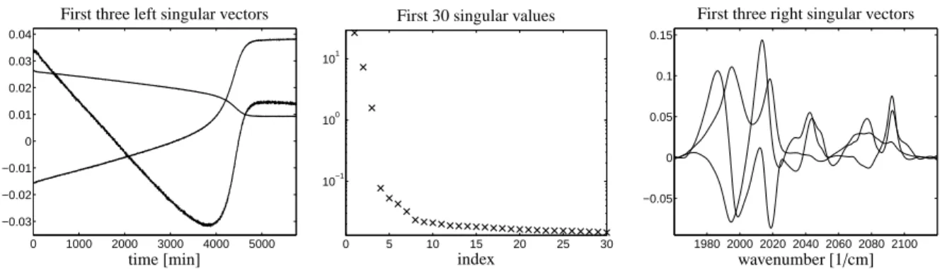
Figure 2: Singular value decomposition of data matrix D from Rhodium-catalyzed hydroformylation. Left: the first three left singular vectors.

Middle: the first 30 singular values in a logarithmic plot. Right: the first three right-singular vectors.

Algorithm 3 Coupling for s₀=s−1.

Ensure: Coupled concentration profilesC(:,1 : s−1)

1: [U,S,V] = svd(D);

2: for i=1:s

4: U(:,i) = -U(:,i);

5: V(:,i) = -V(:,i);

6: end;

7: end;

8: T = A*V(:,1:s);

9: W = T\eye(s-1,s-1);

10: y = null(T);

Each coupled concentration profile is an element of a one-dimensional affine subspace. For each i = 1, . . . ,s−1 a proper interval [ai,bi] with maximal length bi−aiis to be determined which guarantee nonnegative concentration profiles.

11: i = 1; % i = 2; i = 3; ...

12: m = 20;

13: g = linspace(a(i), b(i), m);

14: plot(U*S(:,1:s)*(W(:,i)*ones(1,m)+y*g));

orated techniques. References on the extraction of pure component spectra for trace components with a very low signal-to-noise ratio and their successful confirma- tion, e.g. by DFT computations, are [17] in Sec. 4.4 or [36, 35, 37].

Next we would like to discuss the influence of ran- dom and systematic noise on the results as well as its dependence on the ratio of total absorbance of a certain species to the level of noise. The effects also depend on the used spectroscopic technique.

1980 2000 2020 2040 2060 2080 2100 0

0.01 0.02 0.03 0.04 0.05 0.06 0.07 0.08

wavenumber [1/cm]

Series of spectra

Figure 1: Selection of 34 of k=2621 spectra for the k=2621×n= 664 spectral data matrix D for the Rhodium-catalyzed hydroformyla- tion process.

5.1. Low rank approximation by the SVD

A key step in spectral recovery techniques is the low rank approximation of C and A by using only the s largest singular values and the associated s left and right singular vectors. If the reconstruction error D−U(:,1 : s)Σ(1 : s,1 : s)V(:,1 : s)^T is small, then multivariate curve resolution methods can work very well. However in the presence of systematic noise and if the signal-to- noise ratio for a specific component is not small, then the truncated SVD is not a reliable basis for the reconstruction of the correct solutions [7, 35, 23, 33]. In this case the low rank representation T (:,1 : s)=A(1 : s,: )V cannot reconstruct the spectral data very well as the error A(1 : s,:)−A(1 : s,:)VV^T is not small. Then an application of the complementarity and coupling theory cannot be recommended.

5.2. Trace components with a low signal-to-noise ratio If the noise level is relatively small and the signals of a trace component are of a size comparable to the 6

(7)

noise level, i.e. the signal-to-noise level for this component is large, then a successful strategy is to work with z singular vectors in order to construct a number of s spectra with z > s. Then the matrix T in (2) is a rect- angular s×z matrix and T⁻¹ is to be replaced by its pseudoinverse T⁺, see [35]. For this more general sit- uation the complementarity and coupling theory cannot be applied, since it has only been formulated for square matrices T∈R^s×s.

5.3. Further spectroscopic techniques

Up to now we have successfully applied the complementarity and coupling theory to UV/Vis and FT- IR data, see Section 6 and [27, 28, 31]. Especially for UV/Vis data the size and type of the noise is not in- terfering the computational procedure. However, for FT-IR data a potential baseline correction is a critical step whose proper implementation is crucial for the sub- sequent computations. In principle the complementarity and coupling arguments appear to be useful build- ing blocks for extracting pure component information if proper adscititious information on the chemical system is available. These techniques might be a part of a prospective automatic analysis of mixtures, cf. with the automatic analysis in X-ray powder diffraction [3, 2].

6. Application to the Rhodium-catalyzed hydro- formylation process

In this section the numerical algorithms and program codes are applied to in situ FTIR spectroscopic data from the Rhodium-catalyzed hydroformylation process.

For the experimental details see [15]. Within the spectral interval [1960,2120]cm⁻¹ three dominant active species can be identified; two of the pure component spectra of the three components are known. These are ideal preconditions for the application of the complementarity and coupling theory.

6.1. Spectral data and two pure component spectra A series of k = 2641 spectra were taken from the hydroformylation of 3,3-dimethyl-1-butene with a rhodium/tri(2,4-di-tert-butylphenyl)phosphite catalyst ([Rh]=3·10⁻⁴mol/L) in n-hexane at 30^◦C, p(CO)= 1.0 MPa and p(H2) = 0.2 MPa. Each spectrum is a vector with n = 664 absorbance values in the interval [1960,2120]cm⁻¹. Figure 1 shows 34 of these spectra.

Within this spectral interval the reactant 3,3-dimethyl- 1-butene as well as the hydrido and acyl rhodium com- plexes are the prevailing components, cf. [15]. This statement is supported by the distribution of the singular

1980 2000 2020 2040 2060 2080 2100 wavenumber [1/cm]

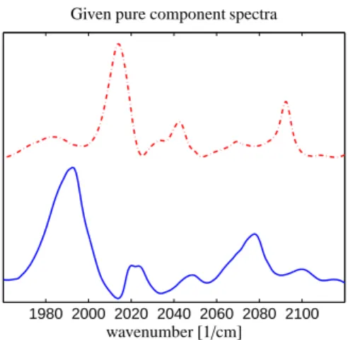
Given pure component spectra

Figure 3: The two known pure component spectra. The olefin (component 1) is shown by a blue line and the hydrido complex (component 3) by a red dash-dotted line.

values. The three largest singular values are character- istically larger than the remaining singular values which are close to zero. Thus we set s=3. Figure 2 shows the singular values together with the left and right singular vectors.

Two spectra of the reaction subsystem are known:

The spectrum of the olefin 3,3-dimethyl-1-butene is available, and the spectrum of the hydrido complex is known. These two specta are shown in Figure 3.

6.2. Application of the complementarity theorem The complementarity theorem can easily be applied.

Two of the three pure component spectra are available so that the simplified complementarity theorem 3.1 can be used. The concentration profile of the third component (acyl complex) is uniquely determined aside from scaling. Algorithm 1 with s =3 results in the concen- tration profile C(:,2) of the acyl complex, see Figure 4.

6.3. Application of the coupling theorem

Since all but one pure component spectra are available, Algorithm 3 can directly be applied. Next we explain the computation of the concentration profile of the olefin. The profile for the hydrido complex can be computed similarly. After the initialization phase a particu- lar solution W of the under-determined system of inho- mogeneous linear equations T W(:,1)=(1,0)^Tis com- puted, see line 9 in Algorithm 3. In Figure 5 UΣW(:,1) is shown by the solid line. Then the null space of T is computed. Figure 5 shows UΣy as a broken line for a y,0 from this null space. The affine linear spaceC⁽¹⁾ in Theorem 3.3 is then spanned by all C(:,1) = UΣz 7

(8)

0 1000 2000 3000 4000 5000 0

0.05 0.1 0.15 0.2 0.25

0 1000 2000 3000 4000 5000 0

1 2 x 103 ⁻⁴

time [min]

Concentration profile C(:,2) of the acyl complex

Non-scaledconcentration Conc.acylcomplex[mol/l]

Figure 4: The application of the simplified complementarity theorem in the form of Algorithm 1 yields the concentration profile C(:,2) nor- malized to maximum 1. Left ordinate shows the non-scaled concentration as resulting from Algorithm 1; the right ordinate shows the absolute concentration of the acyl complex by using a kinetic model [26].

with z = W(:,1)+γy andγ ∈ R. Finally, a real interval forγis to be determined so that C(:,1) satisfies the two restrictions (I. and II.) from Section 3.4. For the given data we getγ∈[a1,b1] =[1.19, 1.98]. (For all otherγeither C(:,1) has negative components or the rank-reduced matrix D−C(:,1)A(i,:) has negative components.)

0 1000 2000 3000 4000 5000

−0.02 0 0.02 0.04 0.06 0.08

time [min]

Affine linear space for C(:,1)

Figure 5: Construction of the affine linear space for C(:,1). All linear combinations of the particular solution cp =UΣW(:,1) (solid line) and the homogeneous solutions ch=UΣy (broken line) span the affine subspaceC⁽¹⁾as given in (3). Then C(:,1)= cp+γchfor feasible values ofγ.

Figure 6 shows the resulting feasible concentration profiles for the olefin. Similarly, the feasible concentration profiles of the hydrido complex are also contained in a one-dimensional affine subspace. Together with the nonnegativity restrictions the remaining profiles are shown in Figure 7.

0 1000 2000 3000 4000 5000 0

0.01 0.02 0.03 0.04 0.05

time [min]

Feasible concentration profiles C(:,1)

Figure 6: Olefin component: Feasible non-scaled concentration pro- files C(:,1) according to the coupling theorem and withγ∈[a1,b1]= [1.19, 1.98].

0 1000 2000 3000 4000 5000 0

0.01 0.02 0.03 0.04 0.05

time [min]

Feasible concentration profile C(:,3)

Figure 7: Hydrido complex: Feasible non-scaled concentration pro- files C(:,3) according to the coupling theorem and which satisfy the two nonnegativity restriction in Section 3.4 are shown by red curves.

6.4. Complete solution

We have shown above that the complementarity and coupling theory with two given pure component spectra uniquely determines one concentration profile and re- stricts the concentration profiles of the remaining two components to one-dimensional affine subspaces. Thus the complete factorization D=CA has still a single de- gree of freedom.

If some kinetic model is added (in the form of a soft constraint), then this remaining single degree of freedom can be removed, see [15, 26] for the details. The resulting factors are shown in Figure 8.

7. Conclusion

The complementarity and coupling theory provides advantageous tools for multivariate curve resolution techniques in order to exploit the mutual dependence 8

(9)

0 1000 2000 3000 4000 5000 0

0.2 0.4 0.6 0.8

0 1000 2000 3000 4000 5000 0

0.2 0.4 0.6 0.8

0 1000 2000 3000 4000 5000 0 0.5 1 1.5 2 2.5 x 10⁻⁴

time [min]

Conc.olefin[mol/l]Conc.olefin[mol/l] Conc.Rhodiumcomplexes[mol/l]

Concentration profiles Concentration profiles

1980 2000 2020 2040 2060 2080 2100 wavenumber [1/cm]

Pure component spectra

Figure 8: Complete factorization of the hydroformylation reaction system. Blue solid line: olefin component, green broken line: the acyl complex, red dash-dotted line: the hydrido complex.

of the partial knowledge of one factor and the resulting restrictions on the other factor. The mathematical background and the proofs of the complementarity and coupling theorems have been presented in [27].

However, it is not evident how these theorems can practically be applied to spectroscopic data. The cur- rent paper fills this gap and makes available short pro- grams inMATLAB which can easily be applied and adapted to the needs of the users. The application of the software and the interpretation of its results have been explained step-by-step. The usefulness of the software is demonstrated for FTIR spectroscopic data from the Rhodium-catalyzed hydroformylation process.

Something which is not considered in this paper is the so-called area of feasible solutions (AFS) and its com- bination with the complementarity theory. The simul- taneous representation of all feasible nonnegative solutions in the form of a spectral AFS and a concentrational AFS is a very helpful and intuitive user interface for the application of the complementarity theory. For further

details see [4, 29, 31].

References

[1] H. Abdollahi and R. Tauler. Uniqueness and rotation ambigui- ties in Multivariate Curve Resolution methods. Chemom. Intell.

Lab. Syst., 108(2):100–111, 2011.

[2] L. A. Baumes, S. Jimenez, and A. Corma. hITeQ: A new workflow-based computing environment for streamlin- ing discovery. pplication in materials science. Catal. Today, 159(1):126–137, 2011. Latest Developments in Combinatorial Catalysis Research and High-Throughput Technologies.

[3] L. A. Baumes, M. Moliner, and A. Corma. Design of a Full- Profile-Matching Solution for High-Throughput Analysis of Multiphase Samples Through Powder X-ray Diffraction. Chem.

Eur. J., 15(17):4258–4269, 2009.

[4] S. Beyramysoltan, R. Rajk´o, and H. Abdollahi. Investigation of the equality constraint effect on the reduction of the rotational ambiguity in three-component system using a novel grid search method. Anal. Chim. Acta, 791(0):25–35, 2013.

[5] O.S. Borgen and B.R. Kowalski. An extension of the multivari- ate component-resolution method to three components. Anal.

Chim. Acta, 174:1–26, 1985.

[6] S.D. Brown, R. Tauler, and B. Walczak. Comprehensive Chemo- metrics: Chemical and Biochemical Data Analysis, Vol. 1-4. El- sevier Science, 2009.

[7] W. Chew, E. Widjaja, and M. Garland. Band-target entropy minimization (BTEM): An advanced method for recovering unknown pure component spectra. Application to the FT-IR spectra of unstable organometallic mixtures. Organometallics, 21(9):1982–1990, 2002.

[8] P.J. Gemperline and E. Cash. Advantages of soft versus hard constraints in self-modeling curve resolution problems. Alter- nating least squares with penalty functions. Anal. Chem., 75:4236–4243, 2003.

[9] A. Golshan, H. Abdollahi, and M. Maeder. Resolution of Rota- tional Ambiguity for Three-Component Systems. Anal. Chem., 83(3):836–841, 2011.

[10] G.H. Golub and C.F. Van Loan. Matrix Computations. Johns Hopkins Studies in the Mathematical Sciences. Johns Hopkins University Press, 2012.

[11] H. Haario and V.M. Taavitsainen. Combining soft and hard modelling in chemical kinetics. Chemometr. Intell. Lab., 44:77–

98, 1998.

[12] J. Jaumot, R. Gargallo, A. de Juan, and R. Tauler. A graphical user-friendly interface for MCR-ALS: a new tool for multivariate curve resolution in{MATLAB}. Chemom. Intell. Lab. Syst., 76(1):101–110, 2005.

[13] J. Jaumot and R. Tauler. MCR-BANDS: A user friendly MAT- LAB program for the evaluation of rotation ambiguities in Multivariate Curve Resolution. Chemom. Intell. Lab. Syst., 103(2):96–107, 2010.

[14] A. Juan, M. Maeder, M. Mart´ınez, and R. Tauler. Combining hard and soft-modelling to solve kinetic problems. Chemometr.

Intell. Lab., 54:123–141, 2000.

[15] C. Kubis, D. Selent, M. Sawall, R. Ludwig, K. Neymeyr, W. Baumann, R. Franke, and A. B¨orner. Exploring between the extremes: Conversion dependent kinetics of phosphite-modified hydroformylation catalysis. Chem. Eur. J., 18(28):8780–8794, 2012.

[16] W.H. Lawton and E.A. Sylvestre. Self modelling curve resolu- tion. Technometrics, 13:617–633, 1971.

9

(10)

[17] C. Li, E. Widjaja, and M. Garland. Spectral reconstruction of in situ{FTIR}spectroscopic reaction data using band-target entropy minimization (BTEM): application to the homogeneous rhodium catalyzed hydroformylation of 3,3-dimethylbut-1-ene using Rh4(CO)12. J. Catal., 213(2):126 – 134, 2003.

[18] M. Maeder. Evolving factor analysis for the resolution of over- lapping chromatographic peaks. Anal. Chem., 59(3):527–530, 1987.

[19] M. Maeder and Y.M. Neuhold. Practical data analysis in chem- istry. Elsevier, Amsterdam, 2007.

[20] M. Maeder and A. D. Zuberbuehler. The resolution of overlap- ping chromatographic peaks by evolving factor analysis. Anal.

Chim. Acta, 181(0):287–291, 1986.

[21] E. Malinowski. Factor analysis in chemistry. Wiley, New York, 2002.

[22] R. Manne. On the resolution problem in hyphenated chromatog- raphy. Chemom. Intell. Lab. Syst., 27(1):89–94, 1995.

[23] K. Neymeyr, M. Sawall, and D. Hess. Pure component spectral recovery and constrained matrix factorizations: Concepts and applications. J. Chemometrics, 24:67–74, 2010.

[24] R. Rajk´o. Natural duality in minimal constrained self modeling curve resolution. J. Chemometrics, 20(3-4):164–169, 2006.

[25] R. Rajk´o and K. Istv´an. Analytical solution for determining feasible regions of self-modeling curve resolution (SMCR) method based on computational geometry. J. Chemometrics, 19(8):448–

463, 2005.

[26] M. Sawall, A. B¨orner, C. Kubis, D. Selent, R. Ludwig, and K. Neymeyr. Model-free multivariate curve resolution combined with model-based kinetics: Algorithm and applications.

J. Chemometrics, 26:538–548, 2012.

[27] M. Sawall, C. Fischer, D. Heller, and K. Neymeyr. Reduction of the rotational ambiguity of curve resolution technqiues under partial knowledge of the factors. Complementarity and coupling theorems. J. Chemometrics, 26:526–537, 2012.

[28] M. Sawall, C. Kubis, D. Selent, A. B¨orner, and K. Neymeyr. A fast polygon inflation algorithm to compute the area of feasible solutions for three-component systems. I: Concepts and appli- cations. J. Chemometrics, 27:106–116, 2013.

[29] M. Sawall and K. Neymeyr. A fast polygon inflation algorithm to compute the area of feasible solutions for three-component systems. II: Theoretical foundation, inverse polygon inflation, and FAC-PACK implementation. Technical report, Univer- sity of Rostock, 2014. Accepted for J. Chemometrics, DOI:

10.1002/cem.2612.

[30] M. Sawall and K. Neymeyr. FAC-PACK: A software for the computation of multi-component factorizations and the area of feasible solutions, Revision 1.1. FAC-PACK homepage:

http://www.math.uni-rostock.de/facpack/, 2014.

[31] M. Sawall and K. Neymeyr. On the area of feasible solutions and its reduction by the complementarity theorem. Anal. Chim.

Acta, 828:17–26, 2014.

[32] R. Tauler. Calculation of maximum and minimum band bound- aries of feasible solutions for species profiles obtained by multivariate curve resolution. J. Chemometrics, 15(8):627–646, 2001.

[33] M. Tjahjono, X. Li, F. Tang, K. Sa-ei, and M. Garland. Ki- netic study of a complex triangular reaction system in alkaline aqueous-ethanol medium using on-line transmission FTIR spec- troscopy and BTEM analysis. Talanta, 85(5):2534 – 2541, 2011.

[34] M. Vosough, C. Mason, R. Tauler, M. Jalali-Heravi, and M. Maeder. On rotational ambiguity in model-free analyses of multivariate data. J. Chemometrics, 20(6-7):302–310, 2006.

[35] E. Widjaja, C. Li, W. Chew, and M. Garland. Band target entropy minimization. A robust algorithm for pure component spectral recovery. Application to complex randomized mixtures

of six components. Anal. Chem., 75:4499–4507, 2003.

[36] E. Widjaja, C. Li, and M. Garland. Semi-batch homogeneous catalytic in-situ spectroscopic aata. FTIR spectral reconstruc- tions using Band-Target Entropy Minimization (BTEM) with- out spectral preconditioning. Organometallics, 21:1991–1997, 2002.

[37] E. Widjaja and Regina K.H. Seah. Application of raman mi- croscopy and band-target entropy minimization to identify mi- nor components in model pharmaceutical tablets. Jo. Pharm.

Biomed. Anal., 46(2):274 – 281, 2008.

10