A theoretical framework for waveguide quantum electrodynamics and its application to resonance energy transfer

A theoretical framework for waveguide quantum electrodynamics and its application to resonance energy transfer

Dissertation

zur Erlangung des akademischen Grades doctor rerum naturalium

(Dr. rer. nat.) im Fach Physik

Spezialisierung: Theoretische Physik eingereicht an der

Mathematisch-Naturwissenschaftlichen Fakult ¨at der Humboldt-Universit ¨at zu Berlin

von

Diplom-Physiker Tobias Sproll

Pr ¨asidentin der Humboldt-Universit ¨at zu Berlin Prof. Dr. Jan-Hendrik Olbertz Kunst

Dekan der Mathematisch-Naturwissenschaftlichen Fakult ¨at Prof. Dr. Elmar Kulke

Gutachter/innen: 1. Prof. Dr. Kurt Busch 2. Prof. Dr. J ¨org Schamlian 3. Prof. Dr. Wolfgang Nolting

Ich erkl¨are, dass ich die Dissertation selbst¨andig und nur unter Verwendung der von mir gem¨aߧ7 Abs. 3 der Promotionsordnung der Mathematisch-Naturwissenschaftlichen Fakult¨at, ver¨offentlicht im Amtlichen Mitteilungsblatt der Humboldt-Universit¨at zu Berlin Nr. 126/2014 am 18.11.2014 angegebenen Hilfsmittel angefertigt habe.

Berlin, den 31. M¨arz 2015

To my parents

I NTRODUCTION & O ^UTLINE

In 1965, Gordon Moore formulated a law [1], which turned out to be of fundamental importance to make computers one of the irreplaceable tools for our modern world. It is stated as follows (in its weaker form of 1975): “ The number of transistors per area in integrated circuits doubles roughly every two years “ As it turned out this was not only true in this technical environment for which is was originally developed but also for example for data rates in communication technology. For many years there was an impressive agreement between predictions and the technological progress in real world. Unfortunately, due to fundamental physical principles, deviations started to become significant in recent years especially in high end applications. On the fabricational side the technical requirements to perform necessary lithographic processes on the 10nm scale get incredibly sophisticated. For example, for the fabrication of state-of-the-art chips one needs mirrors which have a numerical aperture as small as this number which poses major technical problems if one wants to reach even smaller scales. On a more fundamental level we have the problem that if the transistors become even smaller they reach the size of just a few atoms which means that there are non-vanishing tunnel currents between them even if the transistor is switched off. Also the heat production in small electronic junctions starts to become significant which can eventually lead to destruction in integrated circuits. There are different approaches to overcome this fundamental problems:

One promising candidate is based on spintronics, where instead of the electronic degrees of freedom the spin degrees of freedom of solid state systems are manipulated [2]. Techniques for transporting spin polarized currents as well as basic logic elements like spin field effect tran- sistors have already been successfully build and theoretically understood [2, 3]. Nevertheless, there are still problems, for example, due to spin coherence and gate-induced Rashba coupling which have to be resolved before industrial applications become a realistic possibility [4, 3].

Another maybe more straightforward approach would be to essentially keep the electronic based approach, but looking for new materials with more favorable electronical properties. An exam- ple for this direction of research is the replacement of silicon based transistors by counterparts based on graphene [5] or M oS₂ (Molybdenumsulfid) [6], both with their own problems and advantages (for example graphene transistors are already working at frequencies of 10⁵ GHz but on the other hand the missing gap of natural graphene causes profound fabricational prob- lems).

A third possible direction for future computer technology is based on optics, which has the advantage of higher switching times because the speed of light is much faster then the typical velocity of electrons (and of spinwaves). Furthermore, the power consumption is much less because of the missing charging of transmission lines (this is the main source of power loss in conventional computers). It is also worth noting that because of the lack of direct photon- photon coupling at low energies there is always need for an operating medium which is capable of inducing interactions because they are crucial to perform actual computations [7]. There

are already several possible realizations of optical interconnections to transport information between different logical elements for example on the basis of silicon which has the great ad- vantage that the required technologies are already well developed because they are also used in conventional chip production [8]. There are also promising steps forward in the construction of optical transistors relying on nanoantennas or nanoresonators coupled to single molecules or quantumn dots,just to name a few possibilities [7]. Whereas the mass production of computers based on this technology may still be a matter of decades, integrated chips based on a mixture of optical interconnections and electronic transistor are already much closer to enter real life products as was recently demonstrated [9].

Everything we where talking about above was, regardless of its novel physical and techno- logical aspects, dealing with possible new directions in the construction of usual computers by which we mean they are based in principle on well-known Boolean operations. One can now make a step back and ask the question:

Is this sufficient? Or would it be nice to have a computer which can do something more? The answer is affirmative. For example, if we want to simulate a quantum system consisting of N particles we know that the corresponding general quantum state will contain O(2^N) indepen- dent variables and even if N is just of O(10³) which is way smaller then Avogadros constant, this number is bigger than everything we can expect to be handled by an ordinary computer.

To overcome this problem Richard Feynman proposed in 1981 to build a so called quantum computer which makes use of the laws of quantum mechanics to perform calculations in a very different way then we know from a classical computers [10]. The key idea is to use a system ofN qubits to simulate a system ofN particles (this works at least for local quantum systems [11]).

One of the main advantages of this approach is that we can use the principle of superposition, a quantum computer features many (classical) states at the same time which allows us to per- form a huge amount of parallel computations. This phenomenon is called quantum parallelism.

If not only computations are performed by the help of quantum mechanical effects but also information transport and storage we are doing quantum information processing. There are many proposals how to realize this in experiments. Majorana fermion based approaches [12], spintronics [13] or systems predicated on superconductivity [14] are possible (but by no means all) candidates to complete this formidable task, each with its own problems and advantages.

For example Majoranas are not even detected in nature at the time this thesis is written, but on the other hand they are predicted to be quite robust to environmental influences due to their topological protection. For spintronics the situation is reversed, relatively well understood tech- niques to produce the underlying (pseudo) particles are countered by great problems due to quantum decoherence induced by coupling to external degrees of freedom. Another promising and quite old (rough ideas already show up in [10]) route to quantum computing and quantum information processing is making use of quantum optics.

Whereas the 2001 proposal for a scalable linear optical quantum computer consisting only of linear elements like single photon sources, beam splitters or single photon detectors [15] offers the conceptually easiest way to realize optical quantum computation, problems with the exper- imental implementation of scalability still remain to be solved. For this reasons schemes based on non-linear optical effects (for example the Kerr effect) are still a valid alternative [16].

It is clear that because both, the linear as well as the non-linear, optical schemes discussed above are based on a very controlled interaction between light and matter degrees of freedom, it is essential to understand the underlying physical processes in detail.

The purpose of this thesis is to make a contribution to reach this objective in the area of wave- guide quantum electrodynamics which is also a valid candidate for the practical implementation of quantum information processing where the transmission lines are 1-D waveguides and the qubits are realized through two-level-systems which could be suitable atoms or NV centers in diamond, for example [17][18][19].

Outline

We now outline the content of the different chapters of this thesis

In chapter one we discuss the quantization of the electro-magnetic (EM) field with a special emphasis on the correct implementation and interpretation of gauge constraints. We go in some details through the specific example of the Coulomb gauge, because it will be used for all the applications we discuss later on. The second part of this chapter is devoted to light-matter interaction. This includes the discussion of the two most common approximations in the field of waveguide quantum electrodynamics (WQED) the dipole approximation and the rotating wave approximation. Related to this, we will investigate under which specific assumptions we may substitute a particle interacting with an EM field by a simple two level system (TLS). In the last section we introduce WQED. We give an overview of the experimental state of the art in this field and finally construct and motivate the most simple model Hamiltionian emphasizing especially the role of different dispersion relations which will be a key aspect for the rest of the thesis.

The topic of the second chapter is an introduction of quantum field theory (QFT) which is the backbone of the formalism we develop in later chapters for tackling WQED problems. We start with a short overview of how one can include time dependence in quantum mechanics.

We then give a proof of the Gell-Mann Low theorem which is of fundamental importance for developing the perturbative schemes present in most QFT calculations. After a discussion of Wick’s theorem we are ready to develop many concepts by help of an important physical model, the φ⁴ theory, namely self energies, S-Matrices and the linked cluster theorem. We especially emphasize how many calculations can be made transparent and physically understandable by introducing Feynman diagrams.

In the third chapter, we develop a Feynman diagram approach to WQED for a toy model a 1-D waveguide with arbitrary dispersion relation and a two level system. We consider the one excitation as well as the two excitation sub-sector. We then reproduce results obtained by other authors in a much more transparent and compact manner then before. Especially we classify different processes like photon-photon interaction or interaction-induced radiation trapping according to a corresponding classes of Feynman diagrams. Furthermore, we discuss how Fano resonances can be interpreted as a signature of a photon-photon non-linearity. We also discuss in great detail how different choices of dispersion relations give rise to totally different physical results. Especially we show that the usual linearization of the photon dispersion relation isn’t a very good approximation under many circumstances.

In the fourth and last chapter of this thesis we are going to generalize the model systems by adding an additional TLS. We exactly solve the associated perturbation series discussing again the differences which occur for different kind of dispersion relations. We give an in- depth discussion of the particular families of eigenmodes occurring in this system. This is done numerically as well as by a big amount of asymptotic calculations. Afterwards, we give a short overview about fluctuating forces in general but focusing on a specific type, which is related to the so called F¨orster energy. We then show under which circumstances it might appear in our model system and how it can be tuned by the choice of the initial state. Last but not least, we discuss the bound states in continuum also present in our system. We give general conditions for their existence and we show that they have a profound impact on the time dynamics of the TLS. We end this thesis with an conclusion, where we summarize our results and discuss some possible further areas of application for the tools we developed.

A CKNOWLEDGMENTS

First of all, I want to thank Professor Kurt Busch for the hospitality, help, money and continuous support over the last years. Especially I want to highlight the big patience which was necessary to make me finish this work, I know this must be hard from time to time.

Furthermore I want to thank Professor J¨org Schmalian and Professor Wolfgang Nolting to be the external- and second assessor of my PhD thesis, respectively.

Without the help of the other member of the TOP group at MBI and HU I would never have been able to finish this thesis. Even in the darkest times there was always something to laugh about, thank you for that (and many other things)!

A special thanks goes also to Euler-Lagrange who were always a source of great pleasure and inspiration.

Last but not least I want to thank everyone from my family, I owe all of them so much.

C ^ONTENTS

INTRODUCTION & OUTLINE VII

ACKNOWLEDGMENTS XI

1 QUANTIZATION OF THE EM-FIELD AND LIGHT-MATTER INTERACTION 1

1.1 Introduction . . . 1

1.2 A broad perspective on QFT . . . 1

1.3 Quantization of the EM Field . . . 2

1.3.1 Covariant formulation and Gauge Symmetry . . . 2

1.3.2 Quantization in Coulomb Gauge . . . 3

1.4 Light Matter coupling . . . 5

1.4.1 The Dipole Approximation . . . 5

1.4.2 The Rotating Wave Approximation . . . 8

1.5 Waveguide Quantum Electrodynamics . . . 8

1.5.1 Experimental Overview . . . 8

1.5.2 Modelling WQED . . . 9

2 QUANTUM FIELD THEORY AND DIAGRAMMATICS 13 2.1 Introduction . . . 13

2.2 Pertubation theory in QFT . . . 13

2.2.1 The time evolution operator . . . 13

2.3 Gell-Mann Low Theorem . . . 15

2.4 Wick theorem . . . 16

2.5 Green’s functions . . . 17

2.5.1 Types of Green’s functions and connections to perturbation theory . . . 18

2.6 The φ⁴ model as a case study . . . 19

2.6.1 Feynman diagrams in theφ⁴-theory . . . 22

2.7 The self-energy . . . 26

2.7.1 The scattering matrix . . . 27

3 DIAGRAMMTIC APPROACH TOWQEDWITH APPLICATIONS TO THE ONETLSPROBLEM 31 3.1 Introduction . . . 31

3.2 Path integral approach . . . 33

3.2.1 Single excitation sector . . . 36

3.2.2 Two excitation sector . . . 38

3.3 Feynman diagram representation . . . 39

3.3.1 Single excitation sector . . . 40

3.3.2 Two excitation sector . . . 42

3.4 Properties of the Green’s functions in the single-excitation sector . . . 44

3.5 Properties of the Green’s functions in the two-excitation sector . . . 47

3.5.1 Cosine dispersion relation - discrete waveguide . . . 47

3.5.2 Linear dispersion relation . . . 48

3.5.3 Band edge effects . . . 52

3.6 Conclusion . . . 54

4 THE TWO SCATTERER PROBLEM AND FLUCTUATING FORCES 57 4.1 Introduction . . . 57

4.2 The model . . . 58

4.3 Diagramatic solution . . . 59

4.3.1 Preliminaries & Notations . . . 59

4.3.2 The full Green’s function . . . 60

4.4 Analysis of eigenvalues . . . 63

4.4.1 Cosine dispersion relation . . . 63

4.4.2 Linear dispersion relation . . . 71

4.4.3 General existence condition for bound states in the continuum . . . 71

4.5 Dynamics of the TLS for the linear spectrum . . . 73

4.6 F¨orster Energy Transfer . . . 76

4.6.1 Introduction . . . 76

4.6.2 The definition of the F¨orster Energy . . . 77

4.6.3 Calculating overlap integrals via Green’s functions . . . 78

4.6.4 First case-study: One atom excited . . . 79

4.6.5 Second case-study: Entangled states . . . 84

4.7 Conclusion . . . 88

5 CONCLUSION& OUTLOOK 89 5.1 Conclusion . . . 89

5.2 Outlook . . . 91

A ABSORPTION AND EMISSIONGREEN’S FUNCTIONS 95 A.1 Single-excitation sector . . . 95

A.2 Two-excitation sector . . . 96

B EQUAL TIMEGREEN’S FUNCTIONS 99 C TWO-EXCITATION SCATTERING MATRIX 101 D PROOF OF THE GELL-MANNLOW THEOREM 105 E ASYMPTOTICS FOR THE TWO SCATTERER PROBLEM 107 E.1 Energies . . . 107

E.1.1 Energies at small distances . . . 108

E.1.2 Energies atR_c . . . 108

Contents

E.1.3 Eigenvalues at infinity . . . 110

E.2 Residues . . . 111

E.2.1 Residues at infinity . . . 111

E.2.2 Residues at small distances and atRc . . . 116

PUBLICATIONS 120

L ^{IST OF} F ^IGURES

1.1 The two different dispersion relations discussed in the text: A cosine dispersion with width 4J and the two branches or its linearized approximation around

k=±π/2 . . . . 10

1.2 The model system, consisting of a one dimensionl waveguide and a two level system 11 2.1 The free Green’s function and its diagrammatic representation . . . 22

2.2 The four point vertex and its diagrammatic representation . . . 22

2.3 The first diagram in first order perturbation theory . . . 23

2.4 The second diagram in first order perturbation theory . . . 23

2.5 The vacuum diagram in first order perturbation theory . . . 24

2.6 All diagrams in second order perturbation theory. The three in the top row are the vacuum contributions. Additonally the corresponding symmetry factors are shown . . . 24

2.7 Diagramatic visualization of the linked cluster theorem . . . 25

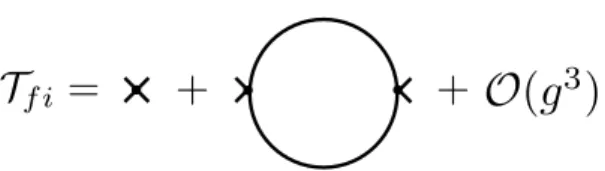
2.8 The the T-Matrix in second order perturbation theory. The small lines indicate the amputated outer legs. All momenta/energy labels are suppressed . . . 29

3.1 Spectral density of the TLS with Ω = 0, U = 1, v = 1 and t= 1 for the linear (black, dashed) and cosine (red) dispersion relation. ω is measured in units of v (t) for the linear (cosine) dispersion relation and the spectral density in units of v⁻¹ (t⁻¹). The spectral density of the cosine band clearly displays the band edges and features spectrally ultra-sharp bound states in the band gaps on either side of the band (when plotting the spectral density for the cosine band, we have introduced an artificial broadening δ = 10⁻⁴ in order to enhance the visibility of the bound states). By contrast, the spectral density for the linear dispersion relation corresponds to a simple Lorentzian. . . 45

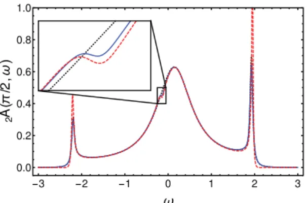
3.2 Two-excitation spectral density ₂A(π/2, ω) (obtained via the Green’s function approach (solid blue) and DMRG (dashed red)) of the TLS with Ω = 0.3 and U = 1 for a tight-binding waveguide with L = 600 discrete sites and cosine dispersion relation (k) = −2tcos(k) (t = 1), together with the corresponding single-excitation spectral density 1A(ω) (black dotted). ω is measured in units of t and the spectral density in units of t⁻¹. In ₂A(π/2, ω), we clearly observe a Fano-resonance just below ω = 0 (see text for details). This Fano-resonance is absent in the single-excitation spectral density of the TLS. When plotting the spectral densities, we have introduced an artificial broadening δ = 0.04 in order to enhance the visibility of the Fano-resonance and to improve numerical convergence. . . 47

3.3 Two-excitation spectral density ₂A(−1, ω) (solid blue) of the TLS with Ω = 1 and U = 1 for a waveguide with linear dispersion relation (k) = μvk and v= 1 considered in the continuum limit, together with the corresponding single- excitation spectral density ₁A(ω) (red dashed). ω is measured in units of v and the spectral density in units of v⁻¹. We have shifted the single-excitation spectral density₁A(ω) byω→ω−vk, so that the maxima of both plots overlap.

The green dotted line is at vk+ Ω/2 and indicates the maximum of ₁A(ω). In

2A(−1, ω), we clearly observe a Fano-resonance atω = 2vk−Ω/2 (black-dotted line) which is more pronounced than for the case of tight-binding waveguide in Fig. 3.2. As in the case of the tight-binding waveguide, this Fano-resonance is absent in the single-excitation spectral density of the TLS. When plotting the spectral densities, we have introduced the same artificial broadeningδ = 0.04 as in the case of the tight-binding waveguide in order to enhance the visibility of

the Fano-resonance and make the graph comparable to that in Fig. 3.2. . . 50

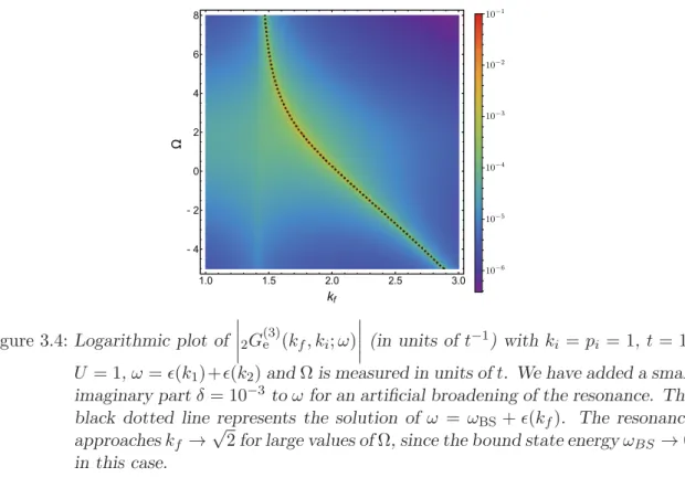
3.4 Logarithmic plot of ²G⁽³⁾_e (k_f, k_i;ω) (in units of t⁻¹) with k_i =p_i = 1, t = 1, U = 1, ω = (k₁) +(k₂) and Ω is measured in units of t. We have added a small imaginary part δ= 10⁻³ toωfor an artificial broadening of the resonance. The black dotted line represents the solution of ω=ω_BS+(k_f). The resonance approachesk_f →√ 2 for large values of Ω, since the bound state energyω_BS →0 in this case. . . 54

3.5 Plot of Res 2G⁽³⁾_e , k₀ (in units of t⁻¹) for two identical initial photons ω = 2(ki), U = 1, t = 1, δ = 10⁻⁴, λ = 10⁻⁶ and Ω is measured in units of t. The black and white lines represent the parabolas Ω = 2(k_i) and Ω = (k_i), respectively. . . 55

4.1 The System . . . 58

4.2 Free Green’s functions . . . 59

4.3 Free Greensfunctions . . . 60

4.4 Pertubation Series for G11, fat lines are full Green’s functions . . . 61

4.5 Self consistent diagrammatic representation ofG11,fat lines are full Green’s func- tions . . . 62

4.6 A sketch of the typical behaviour of the solutions of 4.23 . . . 65

4.7 A sketch of theR-dependent and the R−independent parts off_± . . . 65

4.8 The energy values above the band. Level repulsion is clearly visible for R ≈4. Note that both curves stay finite for R= 0, which is not visible . . . 68

4.9 The energy values below the band. At R =R_c, we can observe how one of the eigenvalues slips out the band. . . 69

4.10 Sketch of different classes of Eigenstates . . . 70

4.11 Sketch of different classes of eigenstates for the linear dispersion . . . 72

4.12 Square Modolus of G12(t) for R= 0 . . . 75

4.13 Square Modolus of G₁₂(t) for R= 0 . . . 76

List of Figures

4.14 The occupations above the band. We observe a minimum atR≈0.7 in the state corresponding to ω₊. Note that by comparing the colors of the lines with Fig.

4.8 we can identify the occupations numbers and the corresponding eigenenergy.

Furthermore the DS atR= 0 which occupation 0.5 is clearly visible . . . 81 4.15 The occupations below the band. At R = R_c we can observe that one of the

states starts to become populated. The two curves cross at point not visible neither in the plot nor in the inset . . . 82 4.16 The occupations below the band for larger distances . . . 82 4.17 The F¨orster energy for the case where the first atom is excited. AtR =R_c there

is a cusp due to the disappearance of one of the polaritonic eigenstates. The potential has a minimum value at R≈4.5 . . . 83 4.18 The occupations above and above the band. a) Above the band only the state|+

couples. b) Below the band the coupling of the two energy eigenstates oscillates in units of R= 1 . . . 86 4.19 The F¨orster potential φ_+,comp for the symmetric state. It is dominated by the

contribution above the bandφ_+,ab, modulated by oscillations which start to fade out forR > R_c . . . 88 5.1 The basic diagram in the two particle subspace for the two scatterer problem . 91

1 ^Q UANTIZATION OF THE EM- ^{FIELD AND}

LIGHT - ^MATTER I ^NTERACTION

We discuss the quantization of the electromagnetic field and light matter interaction

1.1 Introduction

We begin with a short overview of the history of quantum field theory (QFT). Then we discuss the quantisation of the electromagnetic field and especially the role of theU(1)-Gauge symme- try. Later on we will introduce light matter coupling and justify the approximations leading to the standard effective Hamiltonian used in Quantum optics. In the last section we give a brief introduction to the status of experiments in wavequide QED as well as to its theoretical foundations. We thereby obtain the Hamiltonian used throughout the main part of this thesis.

1.2 A broad perspective on QFT

The roots of QFT lie in the realm of particle phyiscs, beginning with works of Heisenberg, Pauli,Jordan and Dirac in the second half of the 1920s [20]. Its first important application was the description of β-decay by Fermi 1934 [21], where the formalism showed its ability to make physically important predictions which are not easily obtained by using standard quantum me- chanics. A period of slow progress followed because of a lack of tools to interpret (infrared and ultraviolett) divergences which are a quite generic feature of QFT. Those problems remained unsolved until the late 1940’s when a new generation of physicists (Schwinger, Dyson, Feyn- man and others) found a solution to this problem by a proper interpretation of the physical constants (mass, electron charge,...), appearing in quantum electrodynamics (QED) as effective parameters which are renormalized by vacuum fluctuations and self energy corrections [22, 23].

A further boost to the field was induced by the ingenious observation of Feynman that one can assign pictorial representations to the complicated mathematical expressions which appear in perturbation theory, the so called Feynman Diagrams [24]. They opened the door for an intu- itive interpretation of QFT and will be one of the main tools of this PhD thesis and will be the

topic of the next chapter. Since that time, QFT was the main driving force in the understanding of the fundamental forces of nature, culminating in the unification of electroweak, electrostrong and electromagnetic interactions by Glashow, Weinberg, Salam and others [25, 26] which is now known as the standard model. Furhtermore QFT has found its way in may areas of theoretical physics, like condensed matter theory [27], statistical physics [28] and also quantum optics [29], partly unifying the theoretical foundations of all these fields.

1.3 Quantization of the EM Field

In this section we mainly follow the script of Tong [30]. We use the following conventions:

Quantities with a lower index, liketμ₁,...,μ_n, transform as rank-ncovariant tensors, objects with an upper indext^μ1,...,μn transform as rank-ncontravariant tensors . The metric tensor is defined as g = diag(−1,1,1,1). Space-time indices are labeled by Greek letters, whereas usual space indices are labeled by Latin letters. Furthermore, Einstein summation convention is imposed.

1.3.1 Covariant formulation and Gauge Symmetry

We start from the classical Lagrangian density of the EM field (we set the source terms to zero) L= 1

2F_μνF^μν (1.1)

where the covariant field strength tensor is given byFμν =∂μAν−∂νAμ (Aμis the four vector potential). Its contravariant counterpart might be obtained by the usual contractions with metric tensors g^μν. Two of Maxwell’s equations are given by the Euler-Lagarange equations:

−∂_μF^μν = 0⇔ ∇ ·E = 0, ∂_tE =∇ ×B (1.2) It turns out that the second pair of Maxwell’s equation follows from the Bianchi identiy

∂_λF_μν+∂_μF_νλ+∂_νF_λμ = 0 (1.3) which can be proven by applying Jacobi’s identity which can be stated for this particular case as [∂λ,[∂ν, Aμ]] = 0,where [,] denotes the Lie bracket. Plugging in the components of the field strength tensor we obtain:

∇ ·B = 0, −∂_tB =∇ ×E (1.4)

Even at this general level, an obvious but profound problem shows up:

Aμ has four components but the photon should only have two degrees of freedom (the two polarisation directions).

How can we resolve this issue?

The first degree of freedom can be eliminated by the fact thatA₀ is static (this follows directly from the anti-symmetry ofFμν). Applying∂ⁱ toF_i0 =Ei we might conclude that

∇²A₀=−∇∂_tA (1.5)

1.3 Quantization of the EM Field

so the time component of the vector potential is uniquely fixed by the three space components.

The second degree of freedom can be eliminated by the inherentU(1) (local) gauge symmetry of electromagnetism. We recall that this means that Fμν is invariant under a transformation of the connection having the formAμ→Aμ+∂μα(x).

We interpret a gauge transformation in the following way:

In contrast to global symmetry, which implies a conserved charge by N¨other’s theorem, the (infinite dimensional and space-time dependent) gauge transformation is a redundancy of the system, or in other words, just a simple relabeling of its physical states.

We can see that this interpretation is useful by looking at the wave equation

g_μν∂²−∂_μν

A^ν = 0 (1.6)

We might observe that the special choice A^ν = ∂^να(x) is a zero mode of the operator and therefore the equation above is non-invertible. This is a problem because that would mean that we can’t distinguish between the solutionsA_ν and A_ν +∂_να(x). Fortunately this problem can naturally solved by just identifying A_ν ≡A_ν +∂_να(x), because this is just of the relabelings of physical states allowed by gauge symmetry. This additional possibility of relabeling the vector potential eliminates another degree of freedom (we fix a gauge by choosing a particular representative forA_ν).

We now have a quick look at two different gauge conditions:

• Lorenz gauge: ∂_μA^μ= 0

This choice has the particular advantage that it preserves the Lorentz invariance of the theory.

It is therefore the preferred choice in high energy physics. It’s drawback is the quite difficult quantization procedure (see [30],[31]) .

• Coulomb gauge: ∇A = 0

This choice has as an obvious drawback of breaking of the Lorentzian invariance. On the other hand it turns out that its quantization is quite straightforward. Furthermore because we will work at quite low energies, we don’t have to take into account relativistic effects and therefore we will work in this gauge throughout this thesis.

1.3.2 Quantization in Coulomb Gauge

In Coulomb gauge the wave equation (1.6) has the simpler form (A₀ = 0 see ( 1.5))

∂²A = 0 (1.7)

using a plane wave decomposition A(x) = _d3k

(2π)²q(k)e^ik·x we see that the Coulomb condtion turns into

q·k = 0 (1.8)

which means that the polarizations q are perpendicular to the direction of motion given by k. Furthermore we observe that due to the vanishing mass of the photons and the on-shell

condition we may fix E =k₀ =(k) where (k) denotes the photon dispersion relation. As a side-remark we might note that photons in free space field theory have a dispersion relation (k) = k but later on we will also deal with photons which travel trough more structured environments, so we include this possibility already at this point. Condition (1.8) suggests that we can decompose q as

q(k) =c₁ζ₁·(k) +c₂ζ₂·(k) (1.9) where ζl·ζm =δlm, ζl·k= 0. This vectors also obey the completeness relation

l

ζ_lⁱζ_l^j =δ^ij −kⁱk^j

k² (1.10)

To show this we observe that the above quantity can be also seen as the projection matrix onto the directions perpendicular tok. The most general form of this projection matrix which respects rotational symmetry is given by P^ij =aδ^ij+bkⁱk^j . The relation P^ijk_j = 0 fixes the constants.

No we are ready to start with the quantisation procedure. We will try to use Ei and Ai

as conjugate variables because they are the two conjugate variables in classical field theory(

∂L

∂(∂_tA)_i =E_i ).

Note that from here on Ai, Ei are always understood as operators until stated otherwise.

Straightforwardly replacing Poisson brackets by commutators yields

[E_i, E_j] = [A_i, A_j] = 0

[Ei, Aj] =−iδijδ(x−y) (1.11) but this would imply (go to momentum space to see that)

[∇ ·E, ∇ ·A] = i∇²δ(x−y) (1.12) which is clearly not consistent with our constraints

∇ ·E =∇ ·A = 0.

We therefore see that our naive quantization procedure is clearly wrong. We don’t go into the details how one does quantization under constraints, which is a very deep and broad field [31]. We choose rather an ad-hoc method, replacing δ_ij →δ_ij−(∇²)⁻¹∇i∇j in (1.11).

[Ei, Ej] = [Ai, Aj] = 0 [E_i, A_j] =−i

δ_ij −(∇²)⁻¹∇i∇j

δ(x−y) (1.13)

Going to momentum space, we may now check that the constraints are correctly implemented.

It is furthermore worth noting that this are exactly the projection operator on the transverse and therefore physical degrees of freedom (1.10).

We now again apply a plane wave decomposition

1.4 Light Matter coupling

A = d³k (2π)³

1 2(k)

l=1,2

ζ_l(k)

a_k,le^ikx+a^†

k,le^−ikx

(1.14)

where the operators a_k,l fulfill the usual Heisenberg algebra

[a_k,l, a_k,s] = [a^†

k,l, a^†

k,s] = 0 [a_k,l, a^†

k,s] = (2π)³δ_rsδ(k−k) (1.15) which induces (E=−∂_tA)

E =−i d³k (2π)³

(k)

√2

l=1,2

ζ_l(k)

a_k,le^ik·x−a^†

k,le^−ik·x

(1.16) With this expressions at hand, we may calculate the Legendre transform of L and find (using the Coulomb condition and settingc= 1)

H = d³x(Ei∂tAi− L) = 1

2 d³x

E²+B²

(1.17) Using (1.16) it follows that

H=

l=1,2

d³k

(2π)³ω(k)a^†

k,la_k,l (1.18)

Note that we already have thrown away an infinite constant _d3kω(k)

(2π)³ which doesn’t affect the dynamics of the system (or normal ordered the Hamiltonian to speak in more technical terms).

We therefore showed that the EM Hamiltonian is equivalent to an ensemble of harmonic oscil- lators. This allows for the useful interpretation that the quanta created and destroyed by a^†

k,l

and a_k,l are exactly the photons.

1.4 Light Matter coupling

1.4.1 The Dipole Approximation

In this section, we want to couple the degrees of freedom of the quantized EM field to matter degrees of freedom. To understand the fundamental principles let’s have a look at a single,

charged particle in anSO(3) symmetric potential coupled to the EM field. We neglect the free field part in what follows because it will not be of any further concern. We rely loosely on [32]

generalizing the arguments for a quantized light field. Note,that for the sake of clarity we don’t write out constants of proportionality here, which is indicated by∼.

The Hamiltonian can be obtained by the principle of minimal substitutionp→p−e A, H = 1

2m

p−e A

2

+φ(|x|) (1.19)

Where φ(|x|) is the potential. Next we omit the diamagnetic term ∼ A² which is legal in many situations because it is suppressed by a factor of 1/c(in Gaussian units). Additionally it doesn’t affect light matter coupling so it is of no concern to us anyways (This term induces also the so called ponderomotive force, important in strong field theory). Furthermore employing the Coulomb condition we get

H = 1

2mp²− e

mAp+φ(|x|) (1.20)

using (1.16) and defining|i/f ≡ |n_i/f, ψ_i/f=|n_i/f|ψ_i/f, the initial/final states composed of a light part|n_i/fand a matter part|ψ_i/f, we see that the overlap matrix elementO_{f i}∼ f|Ap|i may be written as

O_{f i}∼ d³k

l=1,2

f|ζ_l(k)a_k,le^ikxp|i+h.c (1.21) If the size of the particle x₀ is now much smaller then the typical wavelength of our electro- magnetic field we might perform a Taylor expansione^ikx ≈1 +O(ikr) to get

Of i∼ d³k

l=1,2

f|ζl(k)a_k,lp|i+h.c= (1.22) d³k

l=1,2

ζ_l(k)f|a_k,lp|i+h.c (1.23) Note that the argument above is not completely rigorous because we formally integrate over all photon momenta so the Taylor expansion seems questionable. This can be cured by remember- ing that a real photon has a momentum distribution g(k) which is peaked around some value k=k₀ for which we assume that x₀k₀ 1 (in real world system this factor is of 10⁻⁴−10⁻⁵ most of the time ).

Now remembering that [^p_m² +φ(|x|), x] = _m^p we may rewrite (1.22) as O_{f i}∼ d³k

l=1,2

ζ_l(k)n_f|a_k,l|n_iψ_f|d|ψ_i −h.c (1.24)

Here we have introduced the dipole operatord≡ex, Now after reintroducing the constants of proportionality and using again (1.16) we see can show that

1.4 Light Matter coupling

O_{f i}=−ψ_f|d|ψ_in_f|E|n_i (1.25) Now, without loss of generality, let’s chooseζ(k) = (0,0, ζz(k))^T so the position dependent part of the matrix element simplifies to

ψ_f|d|ψ_i=eψ_f|z|ψ_i (1.26) Notice that because our potential is radially symmetric we can decompose our final and initial states as |ψ=|ψlmn =|R(r)nl|Ψlm(φ,Θ) into a radial and an angular part. According to the general theory of selection rules [32] we can fix l= l±1, m= m . Furthermore we find that n_f|a|n_i = √

n_i+ 1

n_f + 1δ_nf+1,ni. Putting everything together, our Hamiltonian can be now written in the form

H= p²

2m² +φ(|x|)−

n_k,n,n,m,l

O_n,n^nk_,m,l|R_n,l+1|Ψ_l+1,m|n_kn_k+1|Ψ_l,m|R_nl|

+h.c. (1.27)

where have absorbed some constants into the matrix element and we have the usual constraints on the ranges of summation forl and m [32].

Let’s discuss this Hamiltonian shortly. Because of the dipole approximation there are only pro- cesses allowed which contain one photon. These are absorption of a photon by the atom, as well as the more exotic creation of an excited state and a photon, which are accompanied by their time reversed counterparts. Due to the conservation of angular momentum all the processes allowed involve the transfer of one quantum of angular momentum (this can be motivated by the fact that a photon is a spin 1 particle ).

To make our model even simpler, let’s assume that our photon is sharply peaked around some frequencyω₀ Furthermore we demand that the atomic transition energies at this frequency are well separated so that we have only one transition which is on resonance with the photon field ω₀ ≈Ω_lmn≡Ω. If these conditions are fullfiled it is sufficent to replace our particle by a simple two level system with energy Ω and states|e(the excited state) and|g(the ground state). A real world example for atoms where this might be a good approximation are the heavy alkaline earth metals caesium and rubidium or nitrogen vacancy (NV) centers in diamond [33]. We get, neglecting irrelevant constants

H = Ω

2σ_z+ d³k

(2π)³(k)a^†_ka_k+ d³k

(2π)³O_k(a_k−a^†_k)(σ₊−σ₋) (1.28)

withσ_z =|ee|+|gg|andσ₊=|eg|, σ₋=|ge|We also used the fact that|n_kn_k+1| ∼a_k and we restored the field part of the Hamiltonian. We note that the overlap element can be chosen to be real, a consequence of theU(1) symmetry of the EM field (a simple phase can be

”gauged out”).

1.4.2 The Rotating Wave Approximation

The purpose of this subsection is to motivate another common approximation, the rotating wave approximation (RWA). Its effect is the replacement

(a_k−a^†_k)(σ₊+σ₋)→a_kσ₊+a^†_kσ₋ (1.29) in (1.28). A first heuristic argument would be that the neglected terms a^†_kσ₊and a_kσ₋ violate the conservation of energy because they create or destroy two excitations (an excited atom and an photon). But as we know this argument is not entirely safe because in quantum mechanics energy conservation is washed out on small time scales. Therefore we need a bit of more rigor.

To do so, we perform a unitary transformation U =e^−iH0t at our Hamiltonian, where H₀ = H_{0,f ield}+H_0,atom . This might be also interpreted as change from Schroedinger to Heisen- berg picture. We furthermore need the following relations e^−iH0tσ_±e^iH0t = σ_±e^±iΩt. and e^−iH0ta⁽_k^†)e^iH0t=e^∓i(k)a⁽_k^†). The left side of (1.29) now reads:

a_kσ₊e^{−i((k)−Ω)t}+a^†_kσ₋e^i((k)−Ω)t−

a_kσ₋e^{−i((k)+Ω)t}−a^†_kσ₊e^i((k)+Ω)t (1.30) we see now, that the phase of the terms in the first line are close to zero if our photon is close to resonance, and therefore they will survive a temporal average. On the other side (k) + Ω≈2Ω and this terms will tend to cancel out during an averaging procedure. Therefore the approximation (1.29) is a valid one as long as the coupling is not too strong . Another way to see this is by using Fermi’s Golden rule. We will come to this later, when we have introduced perturbation theory.

1.5 Waveguide Quantum Electrodynamics

1.5.1 Experimental Overview

Waveguide quantum electrodynamics (WQED) describes a special case of QED where light propagates in a confined geometry. In contrast to cavitiy quantum electrodynamics (CQED) where the light is confined to a certain region of space, WQED supports the propagation of light over large distances in one dimension. It should be mentioned, that many of the systems one can think about can be thought of as coupled cavities where light can tunnel from one cavitiy into the other. In this sense WQED is a generalization of CQED. On the other hand, there are other possibilities to realize WQED. Line defects in photonic crystals [34], ultra-thin glass fibers [35] and coupled ring resonators (The coupling is due to evanescent fields) [36] for exam- ple. One of the points which makes WQED interesting is the fact that the employed boundary

1.5 Waveguide Quantum Electrodynamics

conditions induce very special properties on the propagating photons. The most important one are dispersion relations which can be bounded and curved. This fact can be interpreted that the photons acquire an effective mass, which follows from _m¹_∗ =∂_k²(k) (Remember that this relation only holds around the extrema of the dispersion relation) which also opens up the possibility of a reduced photon group velocity, so we can have a slow light regime [34] and pho- tonic band gaps, even in the presence of disorder [37]. As described in the introduction, WQED has a growing importance in fields like quantum information processing , quantum computing and pump-probe spectroscopy . To obtain an efficient device in this fields it is very important to have quite strong light matter coupling. Possible realizations which offer this feature are ultracold atoms coupled to line defect waveguides as well as well as to nanofibers [38].

Furthermore we want to work with only a few photons to observe quantum mechanical ef- fects such as photon entanglement. Therefore we need single photon sources. This was a great field of experimental research in the past decade, resulting in very different kinds of now avail- able sources including NV centers [39], silicon carbide, which even works at room temperature [40], or silcion quantum dots [41]

1.5.2 Modelling WQED

In this section we want to discuss how to set up the basic model we use together with some slight genralization in the rest of the thesis.

We have discussed light matter coupling as well as quantisation of EM fields ,in quiet some depth, in the last section, so what is left is to specify how exactly we can apply the results we obtained there.

One aspect we want to discuss is, how one can think about a one-dimensional waveguide from a theoretical point of view. We therefore want to discuss two different ways how to realize them.

First, a ultra-thin glasfiber. For this purpose let’s assume that we have cylindrical (lossless) waveguide with radius r. From the theory of classical radiation transport [42] we know as a consequence of the boundary conditions that the allowed modes are quantized in r-direction but have a continuous spectrum inz direction. Furthermore we might observe that the disper- sion relation looks like k_mn,z =

k²−k_mn,r² where mn labels the different allowed modes. It holds thatk_mn,r = ^αmn_r whereα_mn is a zero of a Bessel functionJ_n(x) or its derivative J_n(x).

Therefore if r gets smaller and smaller we might reach a point where only one of the radial modes are allowed to propagate because for all other modes the square root gets imaginary.

This kind of reasoning takes over to the quantum level and that is the way how one should think about one-dimensionality in these systems.

As mentioned in the subsection before, another type of one-dimensional waveguides is built up of coupled ring resonators. We can think of this system as a one-dimensional linear chain with one resonator on each site. If the coupling between neighboring resonators is small, this

Figure 1.1: The two different dispersion relations discussed in the text: A cosine dispersion with width 4J and the two branches or its linearized approximation around k=±π/2

can be modeled as a tight-binding chain with dispersion relation (k) = 2Jcos(k) where J is a measure for the bandwidth of the waveguide (this shape of the dispersion relation can be observed very well in some experiments, see [43]).

The dispersions in both kinds of systems share the main key features, a linear regime as well as a slow light regime and it turns out that this holds also for the other experimental realizations discussed above. Because we are mainly interested in generic features rather than a specific realistic system, it is sufficient to work with the tight binding model discussed above. It has the advantage that it is quite well known (at least in the condensed matter (CM) community) and it is relatively easy to handle from a mathematical point of view. Our field- or photon Hamiltonian therefore reads:

H_ph= 2J dk

2πcos(k)a^†_ka_k (1.31)

where we have performed a field limit, which means that we have dropped an internal length scale given by the lattice constanta. For the purpose of investigating the linear regime we may also occasionally deal with the Hamiltonian

H_ph=v

μ=±

μ dk

2π|k|a^†_ka_k (1.32)

where μ is the chirality and v the group velocity. A plot of both dispersions is given below (Fig. 1.1)

We are now ready too write down a complete model Hamiltonian

1.5 Waveguide Quantum Electrodynamics

Figure 1.2: The model system, consisting of a one dimensionl waveguide and a two level system

H=H_ph+H_a+H_int= (1.33)

dk

2π(k)a^†_ka_k+Ω

2σz+U dk

2πa_kσ₊+a^†_kσ₋ (1.34) where have chosen a uniform coupling in momentum space (O_k ≡ U) and (k) is one of the dispersion relations discussed above. For pictorial representation see (Fig. 1.2)

A first interesting feature of (1.33) is the fact that it supports an additional conserved quan- tity, the particle number

N = dk

2π(k)a^†_ka_k+1

2(σ_z+ 1) (1.35)

which can be readily seen by showing that [H, N] = 0 using the commutation relations of the different involved operators. The appearance of this additional quantum number is a consequence of RWA which neglects processes that increase or decrease the number of particles in the system.

It follows that we can write the Hilbert spaceHas a direct sum of Hilbert spaces with distinct particle number n. H=₀H ⊕1H ⊕2H...⊕nH ⊕...which simplifies many calculations.

2 ^Q UANTUM FIELD THEORY AND

DIAGRAMMATICS

We discuss basics of Quantum Field Theory and diagrammtics

2.1 Introduction

In this chapter we discuss the basic techniques of QFT We start with an overview of how the time evolution of a physical system can be described by the time evolution operator. Then we give a prove of the Gell Mann Low theorem (GMT) which is essential to connect states of an interacting Hamiltonian operator to the states of the corresponding non-interacting system.

This theorem is quite important because it gives the rigorous justification for a perturbative treatment of QFT. We continue by introducing Wick’s theorem which is a necessary tool to perform many QFT calculations, because it allows us to calculate the fundamental objects of any field theory, the correlation functions, in terms of two point correlation functions which is a tremendous simplification. We are then ready to discuss an example of an quantum field theory, namely the φ⁴ model, and show how perturbative calculations work in principle and how they can be simplified and made more intuitive by introducing Feynman diagrams and the corresponding Feynman rules. Along the way we discuss important physical quantities such as the self-energy and the S-matrix which play a major role during the actual research done in this thesis. Furthermore we discuss, within this framework, the so called linked-cluster-theorem which on the one hand reduces the number of relevant diagrams in a given QFT and also gets rid of some of the divergencies which are an intrinsic problem of quantum field theories.

2.2 Pertubation theory in QFT

2.2.1 The time evolution operator

As already suggested by its name, the time evolution operator U(t_f, t_i) is defined to take a Schroedinger state of our quantum system at time t = t_i and evolve it according to the