layered Manganites
probed by optical spectroscopy
Inaugural Dissertation
zur
Erlangung des Doktorgrades
der mathematisch-naturwissenschaftlichen Fakultät der Universität zu Köln
vorgelegt von
Alexander Gößling
aus Bielefeld
Köln, 19. April 2007
Vorsitzender
der Prüfungskommission: Prof. Dr. L. Bohatý Tag der mündlichen Prüfung: 15. Juni 2007
1 Introduction 1 2 Electronic structure of correlated systems and its observation in optics 3
2.1 Onsite properties - lifting the orbital degeneracy . . . . 3
2.2 Intersite properties . . . . 8
2.2.1 Single-band Hubbard model . . . . 8
2.2.2 Mott-Hubbard and charge-transfer insulators . . . . 9
2.2.3 Multi-band Hubbard models . . . . 11
2.2.4 Spin-orbital models . . . . 12
2.2.5 Lattice-mediated orbital interaction . . . . 15
2.3 On- and inter-site excitations and collective modes . . . . 16
2.3.1 Onsite excitations and collective modes . . . . 18
2.3.2 Band-to-band transitions . . . . 21
2.3.3 Excitons . . . . 23
2.3.4 The intensity of an optical transition . . . . 25
3 Spectroscopic techniques 29 3.1 Linear response functions and optical constants . . . . 30
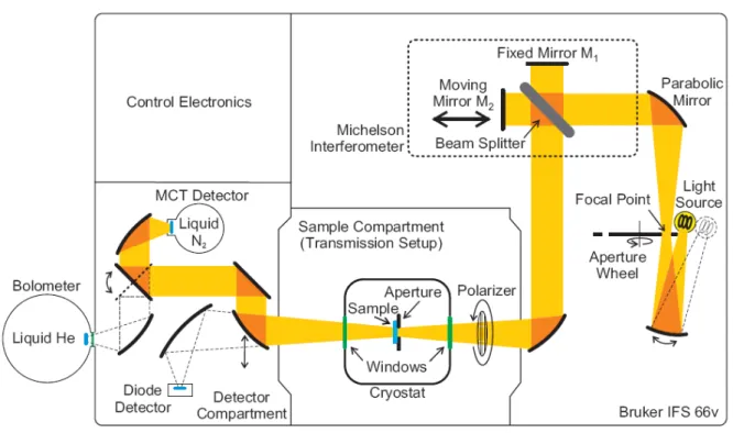
3.2 Fourier-transform spectroscopy . . . . 33
3.2.1 Experimental setup . . . . 35
3.3 Ellipsometry . . . . 38
3.3.1 From Jones-matrix to Müller-matrix formalism . . . . 41
3.3.2 How to measure the Müller matrix? . . . . 43
3.3.3 Experimental setup . . . . 46
3.3.4 Cryostat and bake-out . . . . 47
3.3.5 Calibration procedure and data acquisition . . . . 47
3.3.6 The standard Si wafer . . . . 48
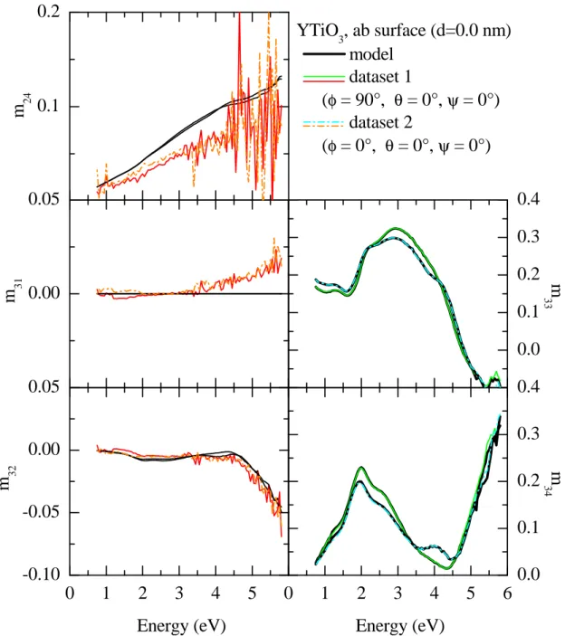
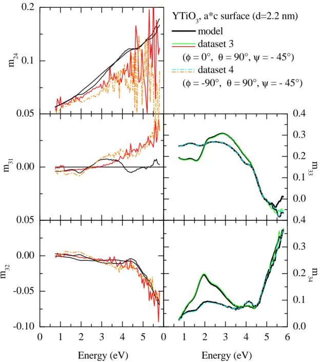
3.3.7 Exemplary data processing for YTiO3 . . . . 48
3.4 Raman scattering . . . . 61
3.4.1 Experimental setup . . . . 64
4 Ellipsometry and Fourier spectroscopy on La1−xSr1+xMnO4 (x=0, 1/8, 1/2) 67 4.1 Physics of manganites . . . . 67
4.2 Details on layered manganites . . . . 75
4.2.1 Crystal structure . . . . 75
4.2.2 Manganese ion in a tetragonal crystal field . . . . 78
4.2.3 Thermal expansion . . . . 79
4.2.4 Electronic structure . . . . 81
4.3 Experimental results . . . . 83
4.3.1 LaSrMnO4 . . . . 83
4.3.2 La1−xSr1+xMnO4 . . . . 88
4.4 Discussion and analysis of LaSrMnO4 . . . . 96
4.4.1 Multiplet calculation . . . . 96
4.4.2 Discussion . . . . 105
4.5 Comparison with the doped compounds . . . . 117
5 Ellipsometry and Raman scattering on YTiO3, SmTiO3, and LaTiO3 125 5.1 Physics of titanates . . . . 125
5.2 Details on titanates . . . . 125
5.2.1 Crystal structure and magnetism . . . . 128
5.2.2 Titanium ion in an orthorhombic crystal field . . . . 130
5.2.3 Electronic structure . . . . 132
5.3 Orbital excitations in LaTiO3 and YTiO3: a Raman scattering study . . . 133
5.4 Electronic structure of YTiO3 probed by ellipsometry . . . . 143
5.4.1 Experimental . . . . 144
5.4.2 Results and Discussion . . . . 145
5.5 Comparison to SmTiO3 and LaTiO3 . . . . 154
6 Conclusions 161 A Appendix 165 Measurement overview . . . . 165
Sample preparation . . . . 166
Temperature at the sample position . . . . 168
Madelung potentials . . . . 169
Unstable surface . . . . 170
Ice layer . . . . 171
Fit of additional data sets of YTiO3 . . . . 172
Bibliography 173 Publications 185 Supplement 187 Danksagung . . . . 187
Offizielle Erklärung . . . . 189
Abstract . . . . 191
Kurzzuammenfassung . . . . 193
2.1 d electron in an octahedral crystal field . . . . 4
2.2 Hybridization . . . . 7
2.3 ZSA scheme . . . . 10
2.4 Lifting the degeneracy by superexchange . . . . 12
2.5 Bond of twoeg electrons . . . . 14
2.6 Orbital liquid . . . . 15
2.7 Sketch of possible optical excitations within a 1D chain . . . . 17
2.8 Franck-Condon principle . . . . 19
2.9 Orbital waves . . . . 20
2.10 Orbiton dispersion . . . . 21
2.11 Mott-Hubbard and charge-transfer transitions . . . . 22
2.12 Excitons in a 1D Mott chain . . . . 23
2.13 Spin-spin correlation function . . . . 25
2.14 Joined spin-orbital correlation function . . . . 28
3.1 Sketch of the Fourier-transform spectrometer . . . . 35
3.2 Sketch of a Michelson interferometer . . . . 36
3.3 Basic geometry of an ellipsometric measurement. . . . 37
3.4 Connection between the measured quantities ψpp an ∆pp and geometrical properties of the polarization ellipse. . . . . 40
3.5 Stokes vector of a RAE system at the detector position. . . . 44
3.6 Sketch of the ellipsometer . . . . 46
3.7 Ellipsometric measurement of the Si standard . . . . 49
3.8 Data processing in ellipsometry . . . . 50
3.9 Measured Müller matrix elements, ab surface (1) . . . . 51
3.10 Measured Müller matrix elements, ab surface (2) . . . . 52
3.11 Measured Müller matrix elements, a∗c surface (1) . . . . 53
3.12 Measured Müller matrix elements, a∗c surface (2) . . . . 54
3.13 Effect of cover layer on measured matrix elements . . . . 55
3.14 Comparison between different cover layers . . . . 56
3.15 Kramer-Kronig consistency . . . . 57
3.16 σ1 of YTiO3 : Comparison to literature results . . . . 59
3.17 Consistency with Reflectance data . . . . 60
3.18 Schematic scattering experiment . . . . 61
3.19 Comparison between Rayleigh and Raman scattering . . . . 63
3.20 Raman scattering setup . . . . 64
4.1 Spin-orbital structure of LaMnO3 . . . . 68
4.2 CE-phase . . . . 69
4.3 Phase diagram of La1−xSr1+xMnO4 . . . . 70
4.4 Phonon spectra of La0.5Sr1.5MnO4 . . . . 71
4.5 Optical conductivity of Eu0.5Ca1.5MnO4 . . . . 72
4.6 Optical conductivity spectra of La1−xSrxMnO3 for x= 0.175 . . . . 73
4.7 Effective carrier concentration of the 2eV feature in LaMnO3 . . . . 74
4.8 Unit cell of La1−xSr1+xMnO4 . . . . 76
4.9 Manganese ion in a tetragonal crystal field . . . . 78
4.10 Lattice constants of La1−xSr1+xMnO4 (x= 0.0, 0.13) . . . . 80
4.11 LDA and LDA+U on LaSrMnO4 . . . . 81
4.12 and σ of LaSrMnO4 . . . . 84
4.13 Change of the optical conductivity of LaSrMnO4 . . . . 85
4.14 Effective carrier concentration Nef f of LaSrMnO4 . . . . 86
4.15 Drude-Lorentz fit of LaSrMnO4 (i) . . . . 87
4.16 Drude-Lorentz fit of LaSrMnO4 (ii) . . . . 89
4.17 Drude-Lorentz fit of LaSrMnO4 (iii) . . . . 90
4.18 Transmission measurements and optical gap for LaSrMnO4 . . . . 91
4.19 of La1−xSr1+xMnO4 as function of doping x. . . . 92
4.20 Optical conductivity σ1 of La1−xSr1+xMnO4 as function of doping x . . . . 93
4.21 Effective carrier concentration Nef f of La1−xSr1+xMnO4 as function x . . . 93
4.22 and σ of La0.87Sr1.13MnO4 . . . . 94
4.23 Transmittance, reflectivity and optical conductivity of La0.5Sr1.5MnO4 . . . 95
4.24 Optical conductivity of La1−xSr1+xMnO4 in comparison to literature data . 96 4.25 Multiplet calculation for LaSrMnO4: a1 . . . . 97
4.26 Multiplet calculation for LaSrMnO4: a2 . . . . 97
4.27 Multiplet calculation for LaSrMnO4: c1 . . . . 98
4.28 Multiplet calculation for LaSrMnO4: c2 . . . . 98
4.29 Energy levels diagrams within a multiplet calculation for LaSrMnO4 . . . . 104
4.30 Sketch of the lowest high-spin transition in LaSrMnO4 . . . . 110
4.31 Sketch of the lowest low-spin transition in LaSrMnO4 . . . . 111
4.32 Effective carrier concentration Nef f of the 2 eV feature in LaSrMnO4 . . . 113
4.33 Additional multiplet excitations for a hole-doped d4 system . . . . 118
4.34 Effective carrier concentration Nef f for La1−xSr1+xMnO4 . . . . 121
5.1 Unit cell of RTiO3 . . . . 126
5.2 Thermal evolution of the lattice constants of YTiO3 and SmTiO3 . . . . . 129
5.3 Crystal-field splitting of a d1 electron in a GdFeO3-distorted crystal . . . . 131
5.4 DOS of YTiO3 from LDA . . . . 132
5.5 Raman spectra of LaTiO3 and YTiO3 . . . . 134 5.6 Raman spectrum of YTiO3 measured at T = 13 K for different laser lines . 135
5.7 Temperature dependence of the Raman spectrum of YTiO3 in (z, z) . . . . 135
5.8 Polarization dependence of the Raman spectra . . . . 137
5.9 Polarization dependence of the Raman spectra of YTiO3, ab plane . . . . . 139
5.10 Polarization dependence of the Raman spectra of YTiO3,a∗cplane . . . . 139
5.11 Comparison Raman spectra vs. σ1 . . . . 140
5.12 Single-orbital excitation in resonant Raman scattering . . . . 140
5.13 Franck-Condon scenario . . . . 142
5.14 Optical conductivity of YTiO3, overview spectrum . . . . 144
5.15 Optical conductivity of YTiO3, temperature dependence . . . . 146
5.16 Configuration-interaction calculation for YTiO3 . . . . 148
5.17 Effective carrier concentration Nef f of YTiO3 . . . . 150
5.18 Calculated excitation energies for YTiO3, Hubbard excitations . . . . 151
5.19 Optical conductivity of YTiO3 from LDA+DMFT . . . . 152
5.20 DOS of YTiO3 from LDA+DMFT . . . . 152
5.21 PES of YTiO3 . . . . 153
5.22 IPES of Y1−xCaxTiO3 . . . . 153
5.23 Exciton formation lowering the kinetic energy . . . . 154
5.24 Comparison of RTiO3 spectra . . . . 155
5.25 Optical conductivity of SmTiO3. . . . 156
5.26 Effective carrier concentration Nef f of SmTiO3 . . . . 158
A.1 Laue picture of SmTiO3 . . . . 167
A.2 Temperature correction . . . . 168
A.3 Unstable surface of LaTiO3 . . . . 170
A.4 Ice layers on YTiO3 . . . . 171
2.1 Multiplet schemes . . . . 6
3.1 Conversion table between optical constants in SI units . . . . 32
4.1 Lattice constants of La1−xSr1+xMnO4 . . . . 77
4.2 Parameters of the multiplet calculation . . . . 99
4.3 Overview of the fit parameters . . . . 99
4.4 Two-center overlap integrals . . . . 108
5.1 Lattice constants and ordering temperatures of RTiO3 (R=Y, Sm, La) . . . 127
5.2 Onsite crystal-field splitting of RTiO3 . . . . 131
5.3 Matrix elements for resonant Raman scattering . . . . 141
A.1 Measurement overview . . . . 165
A.2 Madelung potentials YTiO3 and LaSrMnO4 . . . . 169
A.3 Fit of additional data sets of YTiO3 . . . . 172
The electronic structure is a crucial property of every solid. In semiconductors and conven- tional metals one has a very well established understanding in terms of electronic energy bands and can describe and predict material properties in quite a unique way. In ma- terials with open d shells things become more complicated because the bands are very flat and electrons tend to localize. The theories working well for conventional materials break down. In general these unconventional materials are denoted as correlated electron systems, because one electron strongly influences the other ones.
In correlated materials a variety of interesting phenomena has been found. The most prominent examples are probably the high-temperature superconductivity and the colossal- magneto resistance [1].
In this study we are concerned with the electronic structure of titanates and single- layered manganites. They are prototypical examples where the conventional description in terms of energy bands breaks down: a metallic ground state is predicted for undoped titanates RTiO3 (R-rare earth) and undoped (single-layered) manganites (e.g. LaSrMnO4) but they are both found to be insulating. We will investigate their electronic structure by means of different optical techniques. In addition we are interested in the coupling of electronic degrees of freedom to additional degrees of freedom like the spin or the lattice.
A competition of those is a generic property of a correlated electron system.
Optical spectroscopy has been proven to be a powerful tool for investigating the elec- tronic structure. One measures excitations from the ground state of the system to the excited states. In a non-correlated system the optical spectra represent the folding of the unoccupied and occupied density of states. In correlated materials, electrons strongly influ- ence each other which makes this folding procedure not uniquely applicable. Additionally optical spectroscopy can probe the coupling of the electronic structure to different degrees of freedom [1]. One can for example observe changes in the optical response at several eV (∼ 12000 K) when the system changes its magnetic state on a meV scale (∼ 12 K).
The first (major) project in this thesis deals with the investigation of these spin-controlled bands [2], which are studied as function of temperature and polarization.
In a second project we investigated excitations below the optical gap by means of Raman spectroscopy1. Here, the goal is to get information on the nature of the underlying ground state, which has been discussed controversially in the literature [3–16].
This thesis is organized as follows: In the second chapter we will give a brief overview on correlated electron systems and introduce different models suitable for their description, e.g. the Hubbard model and extensions of it. In the second part we will discuss which
1in collaboration with C. Ulrich and B. Keimer from the Max-Planck Institute in Stuttgart
excitations are expected in a correlated material and how they can be detected by optical spectroscopies. In the third chapter we will present the experimental techniques used in this work: Fourier-transform spectroscopy, Raman spectroscopy and ellipsometry. Since the ellipsometer has been put into operation by my colleague C. Hilgers and myself we will focus on that topic. We are interested in properties down to liquid-He temperatures.
Therefore, it was the major experimental issue to get the system running down to these temperatures. In chapter four the single-layered manganites are introduced, i.e. the system La1−xSr1+xMnO4 forx= 0.0, 0.13, and0.5. We present the results from Fourier-transform spectroscopy and ellipsometry and give a detailed analysis of the electronic structure of this system in terms of multiplets. We focus on the undoped compound withx= 0.0since this is the starting point for a deeper understanding of the whole series. In chapter five we first give the status of the field in the titanates, especially YTiO3, SmTiO3, and LaTiO3, which have been investigated in this thesis. We proceed with the results from Raman spectroscopy, where we studied the orbital excitations on LaTiO3 and YTiO3. The last part of this chapter deals with the electronic structure of the three titanates mentioned above. The excitation spectrum is measured by spectroscopic ellipsometry. Here, we concentrate on YTiO3 because we find evidence for an excitonic resonance (Mott-Hubbard exciton) in this compound. Again we will give an assignment of the peaks observed in terms of multiplets. We end with a final conclusion and some additional information, like sample preparation, etc. in the appendix.
systems and its observation in optics
Optical spectroscopy can cover a wide energy range with high resolution. In this thesis we use different techniques, in particular Raman, Fourier, and ellipsometric spectroscopy to investigate strongly correlated electron systems. More specifically, we will focus on the electronic structure of these systems and its relation to the magnetic, orbital and vibrational degrees of freedom.
This chapter is organized as follows: we will start with the onsite properties of a transition-metal ion. In the next section we will discuss different models applied to corre- lated materials, in particular the Hubbard model and different spin-orbital models. The chapter will end with a brief overview of the excitations in a correlated material and their observation by optical spectroscopy.
2.1 Onsite properties - lifting the orbital degeneracy
The knowledge of the onsite orbital properties is crucial for a proper understanding of a solid. Since we are dealing with transition-metal oxides, it is often sufficient to analyze the properties of the magnetic ions, in the case that the rare-earth ions as well as the oxygen ions have closed shells. Consider for example the compound YTiO3 with Y3+ = [Kr]4d0, Ti3+ = [Ar]3d1, and O2− = [He]2s26p6 or LaSrMnO4 with La3+ = [Xe]5d0, Sr2+ = [Kr]5s0, Mn3+ = [Ar]3d4, and O2−=[He]2s26p6, where the magnetic ions with open shells are Ti3+
and Mn3+. Moreover, the onsite orbital energy scale is often comparable to the intersite exchange interactions which gives rise to a competition. Additionally the orbital properties can be regarded as a kind of preselection for the formation of an electronic band: the band will have the same symmetry as the orbitals forming this band. Orbitals are therefore the basic building blocks of different bands, e.g. the "valence" and "conduction" band. There are three effects which can lift the onsite orbital degeneracy (exchange mechanisms will be discussed below): steric effects, the Jahn-Teller effect, and spin-orbit coupling. All of these effects can be described by crystal-field theory which will be discussed briefly.
In the perovskites, steric effects are caused by a mismatch of ionic sizes. This will lead to distortions and rotations (away from a cubic arrangement). The magnetic ion is surrounded by an electric field produced by the charges of the ligands which lifts the degeneracy of certain energy levels.
Figure 2.1: For an octahedral crystal field which can be produced for example by a ligand-oxygen cage the energy levels of ad1 system are split intot2g ≡(dxy, dxz, dyz)and eg≡(dx2−y2, d3z2−r2) levels. The energy difference between these levels is10Dq.
In addition to simple steric effects a possible reason for the lifting of the degeneracy can be found in the Jahn-Teller effect. The theorem of Jahn and Teller states that "any non- linear molecular system in a degenerate electronic state will be unstable and will undergo distortion to form a system of lower symmetry and lower energy thereby removing the degeneracy" [17]. Presuming Hund’s rules are not violated, a cubic d3, d5, and d8 will not show a Jahn-Teller distortion, because for an e.g. d5 system all d orbitals are occupied and thus no orbital degeneracy is present (the same is true for d3 and d8). If the Jahn- Teller effect is the dominating mechanism a strong coupling to the lattice is expected, i.e. a mixing of the orbital and lattice degrees of freedom.
A further source for lifting the degeneracy is the spin-orbit coupling. However, for RTiO3 and (La,Sr)2MnO4 this is a rather small correction of the order of ∼50 meV [8, 18]. One could say, that the orbital moment is almost quenched. The natural limit for the lifting of degeneracy is the Kramers degeneracy.
Crystal-field theory
In the so called crystal-field theory [19–21] the local properties of magnetic ions can be properly treated. The starting point, of course, is the central magnetic ion which is placed in the potential of all surrounding ligands. One may assume that the charge distribution on each ligand is point-like, e.g. for the case of YTiO3 the Ti ion with charge3+ will be placed in the origin. It will be surrounded by the O ions with charge 2−, the Y ions with charge
3+, and additional Ti ions. In order to obtain the Madelung potential at the origin, the summation of all Coulomb contributions is carried out here up to infinity, half in real, half in reciprocal space (Ewald summation)1. These calculations can be found in the appendix
1The parameters of the Madelung potential have been calculated with a program written by M. Haverkort [8].
for the materials discussed later on. Whether the lattice distortions are caused by steric effects or the Jahn-Teller effect can not be unraveled using crystal-field theory, since the observed crystal structure has to be used as an input. If necessary, one can treat spin-orbit coupling as a further perturbation on top of the electrostatic effects. As discussed above we will omit spin-orbit coupling due to its comparably small magnitude.
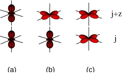
As an example, consider ad1electron in a cubic crystal field as indicated in Fig. 2.1. This cubic crystal field can e.g. be produced by an oxygen octahedron as found in the perovskite structure. The five d orbitals are split into t2g and eg orbitals. The energy difference is commonly denoted by 10Dq. The lobes of the t2g orbitals point towards the median line between two O ions, while those of the dx2−y2 (eg) orbital for example point directly onto the oxygen ions. Therefore, the t2g orbitals are lower in energy because electrons can better avoid each other. For crystals with lower symmetries the degeneracy will be further reduced. For LaSrMnO4 one finds tetragonal symmetry, while for RTiO3 (R - rare earth) orthorhombic symmetry has been reported [7, 22, 23]. In the latter case the degeneracy of alldlevels will be lifted. The corresponding level diagram will be shown in chapters 4 and 5.
Multiplets
So far, our discussion is only correct as long as only one electron is put into the crystal- field levels. For more than one electron, one has to consider the whole multiplet structure.
Because of the antisymmetry of the fermionic wave function, the two-electron wavefunction is not simply a product of two single-electron wavefunctions. This is taken into account by using the Slater determinants. The new basis functions in the cubic case are superpositions ofeg andt2g single-electron functions (configuration mixing) [20]. For ad2system there are 45 basis functions (10 possibilities for the first electron times 9 possibilities for the second electron - divided by two in order to tackle double counting), 120 basis states for d3, 210 for a d4 system, and so on. In addition to the crystal-field parameter Dq for the t2g −eg splitting in the cubic case, one has to take theSlater integralsF0,F2, and F4 into account [1, 19]:
Fk =e2 Z ∞
0
r12dr1 Z ∞
0
r22dr2 r<k
r>k+1 R3d(r1)2R3d(r2)2 (2.1) whereR3d represents the radial wavefunction and r< (r>) the minimum (maximum) value of r1 and r2. This set of parameters describes the repulsion energy between two electrons which are placed on one ion. The definition of the full crystal-field Hamiltonian can be found e.g. in Refs. [18–20]. Alternatively to the Slater integrals F0, F2, and F4, one can use either another set of Slater integralsF0,F2, andF4 or theRacahparametersA,B, and C. The conversion rules are given in Tab. 2.1. Starting from the full multiplet, as presented above, there exist several simplifications which are commonly used in the literature. This is an important issue when comparing for instance values of Hubbard U from different publications. Different schemes lead to different values of U. Here a brief overview:
Table 2.1: Conversion of different multiplet schemes [18–20].
Slater integrals F0 =F0, F2 = 491F2, F4 = 4411 F4 Racah parameters A=F0 −44149F4, B = 491F2− 4415 F4, C = 44135F4 Simple scheme Usimple=F0, JHsimple= 141(F2+F4) Kanamori scheme UKanamori=F0+494 F2+ 44136F4, JHKanamori= 2.549F2+ 22.5441F4
Multiplet average Uav =F0 −44114(F2+F4)
• Simple scheme - In the simple scheme two electrons always repel each other with an energy Usimple regardless in which orbital they reside. If the spins of these two electrons are parallel one gains an energyJHsimple. The advantage of the simple scheme is that one can estimate the energy of a many-electron state just by counting the pairs.
Every pair gets an energy Usimple in case of antiparallel spins and Usimple−JHsimple in case of parallel spins. Consider for example four electrons in a S = 2 state.
One finds six pairs with parallel alignment, which results in an energy of 6Usimple− 6JHsimple (for Dq = 0). The parameters of the simple scheme can be related to the Slater integrals as indicated in Tab. 2.1. The disadvantage of the simple scheme is that both multiplet energies and multiplicities differ sometimes significantly from the full multiplet calculation (see Ref. [18]). However, we will use the simple scheme occasionally in order to get rough estimates of multiplet energies.
• Kanamori scheme- The Kanamori scheme extends the simple scheme in the following way: the parameterUKanamorimeasures the electron repulsion of electrons in the same orbital, while the repulsion is reduced to UKanamori−2JHKanamori if electrons reside in different orbitals (regardless their spin). UKanamori and JHKanamori have of course a different meaning when comparing to the simple scheme. Their relation to the Slater integrals can be read from Tab. 2.1. Consider again the above example of four electrons in anS = 2 state (forDq= 0): the energy reads6UKanamori−18JHKanamori. The Kanamori scheme conserves more of the multiplet character than the simple scheme.
• Multiplet average - This is not a scheme. We just wanted to note that the value of Hubbard U is often given as an average Uav over all multiplets. The relation of Uav to the Slater integrals is also given in Tab. 2.1.
Figure 2.2: Sketch of the σ-bonding dx2−y2 (left) and the π-bonding dxy orbitals (right). For the anti-bonding configuration the phases of all oxygens have to be inverted.
Hybridization
A further improvement of the crystal-field theory is to allow for hopping from the central transition-metal ion to its ligands. In titanates and manganites these ligands are oxygens, i.e. one has to considerporbitals. Depending on the overlap, there will be a sizable admix- ture of thepwavefunctions. This is commonly denoted byα1|dni+α2|dn+1iLstates where
|dn+1iL is a ligand-hole state. However, the symmetry of the original |dni wavefunctions will not be changed. This can be seen in Fig. 2.2(left) for the case of the |d1i = dx2−y2 orbital. This orbital can only hybridize with combinations of the ligands having the same symmetry, i.e. an orbital of the form |d2iL = 12(−p1,x+p3,x+p2,y −p4,y). The overlap between all kinds of orbitals is tabulated in Refs. [24, 25]. The energy levels obtained from a purely ionic picture will change when hybridization is switched on. As a rule of thumb the t2g-eg splitting is increased by a factor of two as shown for the titanates in Refs. [9, 26, 27]. This is quite obvious because the eg orbitals point with their lobes to- wards the oxygen neighbors and will thus be more affected by hybridization than the t2g orbitals. In chapter 5, we will show some results from configuration-interaction calcula- tions, taking the hybridization to neighboring oxygen ions properly into account. For the manganites discussed in chapter 4 we carried out crystal-field calculations and used the crystal-field parameters in an effective manner. We did not use the results from an Ewald summation (see above) but assumed that the effective crystal-field parameters contain a covalent part. As mentioned above, this procedure is justified since the hybridization does not change the symmetry of the wavefunction considered. Due to the different screening the value of Hubbard U will depend on whether covalency is included or not. We will discuss this issue in more detail later on.
2.2 Intersite properties
2.2.1 Single-band Hubbard model
In the description of transition metals with open d shells, band theory (LDA2) fails in describing the electronic properties. At half filling these materials are metals within the LDA, although they are found to be insulators in experiments. The failure of LDA stems from the simplification to a single-electron picture. This approximation works pretty well in ordinary semiconductors, but is not justified in the case of correlated systems, where electrons strongly influence each other. The inclusion of the onsite electron-electron in- teraction can repair the discrepancy between theory and experiment. The most simple approach is the single-band Hubbard model [28]. The system Hamiltonian can be written as follows:
H =−t X
hi,ji,σ
(c†iσcjσ +h.c.) +UX
i
ni,↑ni,↓ (2.2)
Here, niσ≡c†iσciσ is the number operator and c†iσ (ciσ) creates (annihilates) an electron on lattice site i with an a spin σ =↑,↓. The summation is carried out over nearest neighbors hi, ji. The first term of the Hamiltonian means that an electron can decrease its kinetic energy by changing its position with an energy gaint. The second term in the Hamiltonian represents the energy of a double occupancy which is denoted by U. At half filling the movement of an electron will of the one hand gain the energyt but on the other hand the electron is hindered by the repulsion U. The singly occupied sites will form the so-called lower Hubbard band (LHB), while the doubly occupied sites form the upper Hubbard band (UHB). The band width W = 2zt is determined by the size of the hopping t and the co- ordination number z. In the limit U/t →0, the system is metallic because the LHB and UHB overlap and are half filled. In the other limit U/t → ∞ it is an insulator because one finds only one electron per site. The energy cost for a double occupancy is very high, making the electrons immobile. This means LHB and UHB are far away from each other.
Interestingly, one can drive a system from a metallic to an insulating state by changing the size of U/t. Regarding the magnetic properties, the insulating state (t U) of the single-band Hubbard model favors antiferromagnetic arrangement of neighboring spins, because in this case electrons can gain the antiferromagnetic superexchange J = 4t2/U, while in the ferromagnetic case the virtual hopping is blocked by Pauli’s exclusion prin- ciple. The antiferromagnetic arrangement favored in the Hubbard model is described by the Goodenough-Kanamori-Anderson rule for180◦-superexchange. Formally the Hubbard model can be mapped on an effective spin model, which is known as the Heisenberg model
H =JX
hi,ji
Si·Sj (2.3)
2Local Density Approximation.
Within this model, low-energy excitations (∼ meV) such as spin waves can be described3. When simulating real materials with opendshells in more detail, the one-band Hubbard model may give erroneous results because "one-band" corresponds to a single orbital, strictly speaking to an s orbital. The model parameters t and U are of effective nature since real hopping paths have to be integrated out. Excited orbital states on each site are omitted within the single orbital picture and interesting phenomena which arise from degenerate orbitals are not captured. However, the character of the charge excitation gap can be reproduced quite well for lighter transition metals (Ti, V) but not for the heavier ones (Co, Ni, Cu) because the oxygen ligands are not included explicitly.
2.2.2 Mott-Hubbard and charge-transfer insulators
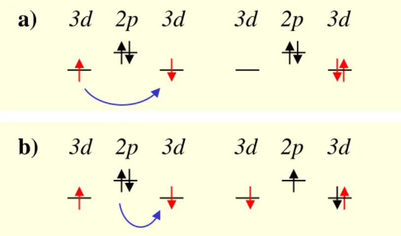
One extension to the single-band Hubbard model is the pd model [30]. It includes one or several oxygen orbital(s) in addition to the transition-metal orbital. This model is widely used for the description of the CuO2 planes of high-Tc cuprate systems. For our purpose, the extension leads to a classification scheme for strongly correlated systems, known as the Zaanen-Sawatzky-Allen scheme [29]. In addition to the parameters t and U, the charge transfer energy∆is taken into account: ∆ = p−dwheredis the energy of the transition- metaldorbital andp the energy of the oxygenporbital. Two kinds of excitations are now possible: one electron can be transferred between two transition metals, or one electron can be transferred from an oxygen ion to a transition metal. Depending on which excitation is lower in energy, i.e. if U or ∆ is larger, the insulator is called Mott-Hubbard insulator or charge-transfer insulator. The gap formed in this insulating state for an n-electron system is given by the many-body groundstate En and the ionic states given by En+1 and En−1:
Egap =En+1+En−1−2En (2.4)
As an example we will calculate Egap for a Mott-insulating chain of N equal sites filled with n electrons. The one-electron energy is given by E0. Thus the ground-state energy at one site is En = nE0 +n(n + 1)/2 U. The term n(n + 1)/2 U counts the onsite correlations for every electron pair. If one electron is added to one site, one obtains En+1 = (n + 1)E0 + (n + 1)(n + 2)/2 U. If one electron is removed one finds En−1 = (n−1)E0+ (n−1)n/2U. Substituting this into Eq. 2.4, the gap results in Egap=U.
We will now discuss the ZSA scheme in more detail, see Fig. 2.3. Apart from the parametersU and∆, one has to take a finite band width of thedandpbands into account.
Roughly speaking, the diagram is split into two regions: for∆< U the electronic structure is dominated by the oxygen band (charge-transfer type) and for ∆ > U by the upper 3d band (UHB). In the first case (panel b) the gap is set by ∆, in the latter case (panel d) by U. Including a finite bandwidth an insulating state will not be formed under all circumstances but a metal can exist either in the charge-transfer or in the Mott-Hubbard region: if the band width of the d band Wd is larger than the onsite repulsion U, a d
3Transformation between Eqs. 2.2 and 2.3 [1]:
Si+=c†i,↑ci,↓,Si−=c†i,↓ci,↑, and Siz=12(ni↑−ni↓)
2p 3d
U < Wd< ∆ Εgap= 0
2p
Wd < U < ∆ Εgap= U - Wd 2p
Wpd< ∆< U Egap= ∆ −Wpd
3d 3d
3d 3d
3d
3d
3d
Wd
∆ U
Wd
∆< Wpd < U Egap= 0
∆ U
c) d metal
2p
UHB
LHB
d) MH insulator
∆
U
a) p metal
∆
U Wpd
b) CT insulator
Wpd
EF
Figure 2.3: Zaanen-Sawatzky-Allen (ZSA) scheme. The interplay of the Coulomb repulsion U, the charge-transfer gap ∆, and the bandwidth W gives rise to different kinds of metallic and insulating states. Note, that Wpd = 12(Wp +Wd). The top panel is the original diagram from Ref. [29], while the cartoon illustrates the four main parts in a band-like picture. However in the cartoon representation the hybridization is neglected in order to be more illustrative.
metal is formed in the Mott region because LHB and UHB overlap (panel c). A similar argumentation leads to a p metal in the charge-transfer region (panel a). Additionally there are some intermediate regions in the ZSA scheme. For their discussion we refer to the original paper.
2.2.3 Multi-band Hubbard models
A generalization of the pd model is the multi-orbital Hubbard model, which allows for different (degenerate) orbitals on each site. The degenerate case is relevant for quasi- cubic systems because here the orbital degree of freedom is not fully quenched, contrary to systems with e.g. large crystal-field splitting [1, 31, 32]. The system Hamilton reads as
H = X
hi,ji σ,α,α0
tααij 0(c†iσαcjσα0 +h.c.) + X
i,α,α0 σ,σ0
(1−δαα0δσσ0)Uαα0niσαniσ0α0
+ X
hi,ji α,α0,σ,σ0
Vijαα0niσαnjσ0α0 − X
i,α,α0 σ,σ0
JHαα0Siα·Siα0(1−δαα0) (2.5)
here spin operators are defined as:
Siα+ = Siαx +iSiαy =c†iα↑ciα↓
Siα− = Siαx −iSiαy =c†αi↓ciα↑
Siαz = 1
2(niα↑−niα↓) (2.6)
Againniσ≡c†iσαciσα is the number operator, c†iσα (cjσα) creates (annihilates) an electron in the orbital α on site i with spin σ =↑,↓. The hopping tααij 0 is now depending on the orbitals and the lattice sites, and also Uαα0 depends on the orbitals (this corresponds to the full multiplet, see Sect. 2.1). Additionally a nearest-neighbor interaction Vijαα0 is now included in order to capture charge-ordering phenomena. This interaction will be of relevance for the formation of excitons which will be discussed later on. Furthermore an intrasite exchange, the Hund’s-rule coupling, JHαα0 is also incorporated. Electrons in two different orbitals with parallel spins are lower in energy than those with antiparallel spins due to Pauli’s exclusion principle.
Due to the large number of possible states, these models require tremendous computa- tional effort. The continually growing computer capabilities made it possible to study this kind of models for real systems exploiting e.g. LDA+DMFT4 [10, 11, 33, 34].
![Figure 4.3: Phase diagrams of La 1−x Sr 1+x MnO 4 . (a) x = 0.0 −1.0 region: from X-ray scattering (• [137]), neutron scattering ( [137] and ♦ [138]), magnetometry ( [139]) and muon spin rotation (](https://thumb-eu.123doks.com/thumbv2/1library_info/3700146.1505966/82.892.158.734.179.831/figure-phase-diagrams-scattering-neutron-scattering-magnetometry-rotation.webp)
![Figure 4.4: Phonon spectra of La 0.5 Sr 1.5 MnO 4 as a function of temperature. (a) Reflectivity data [144] and (b), (c) Raman data [145]](https://thumb-eu.123doks.com/thumbv2/1library_info/3700146.1505966/83.892.172.722.171.487/figure-phonon-spectra-mno-function-temperature-reflectivity-raman.webp)
![Figure 4.6: Optical conductivity spectra of La 1−x Sr x MnO 3 for x = 0.175 [154]. The ferromag- ferromag-netic transition temperature is T c =240 K.](https://thumb-eu.123doks.com/thumbv2/1library_info/3700146.1505966/85.892.285.619.169.541/figure-optical-conductivity-spectra-ferromag-ferromag-transition-temperature.webp)
