Spin and orbital degrees of freedom in transition metal oxides and oxide thin films studied by soft x-ray absorption spectroscopy

Spin and orbital degrees of freedom

in transition metal oxides and oxide thin films studied by soft x-ray absorption spectroscopy

Maurits Haverkort

Spin and orbital degrees of freedom

in transition metal oxides and oxide thin films studied by soft x-ray absorption spectroscopy

Inaugural - Dissertation zur

Erlangung des Doktorgrades

der Mathematisch-Naturwissenschaftlichen Fakult¨ at der Universit¨ at zu K¨ oln

vorgelegt von Maurits W. Haverkort aus Swifterbant, Nederland

K¨ oln 2005

Prof. Dr. T. Hibma Prof. Dr. S. Bl¨ ugel

Tag der m¨ undlichen Pr¨ ufung:

07.06.2005

arXiv:cond-mat/0505214

Contents

1 Introduction 1

1.1 How to measure orbital occupations . . . . 2

1.2 Interpretation of x-ray absorption spectroscopy . . . . 2

1.3 The importance of full multiplet theory . . . . 5

1.4 Scope . . . . 13

2 X-ray absorption spectroscopy 17 2.1 One-electron theory . . . . 19

2.2 Excitons . . . . 21

2.3 Multiplets and selection rules . . . . 26

2.4 Polarization dependence . . . . 33

3 Cluster calculations 43 3.1 Constructing the basis . . . . 44

3.2 Many-electron wave-functions . . . . 44

3.3 Filling in the Hamilton matrix . . . . 45

3.4 One-electron Hamilton Operators . . . . 45

3.4.1 Crystal Field . . . . 46

3.4.2 Covalency . . . . 51

3.5 Two electron Hamiltonian Operators, electron-electron interaction 52 3.6 Spectroscopy . . . . 52

4 Sum-rules 55 4.1 Summery . . . . 64

5 Magnetic versus crystal field linear dichroism in NiO thin films Phys. Rev. B 69, 020408 (2004) 67 6 CoO 75 6.1 Crystal and magnetic structure of cobalt oxide. . . . 77

6.2 Experimental setup . . . . 78

momentum, and exchange coupling. . . . . 85 6.5 Linear dichroism; orbital occupation and spin direction. . . . 87 6.6 Spin direction in thin films of CoO under tensile or compressive

strain . . . 100 6.7 Electronic structure of CoO . . . 102 6.8 Conclusion . . . 107 7 Aligning spins in antiferromagnetic films using antiferromag-

nets 109

8 The spin-state puzzle in the cobaltates 117 8.1 Stabilization of the intermediate-spin state within cluster calcu-

lations . . . 121 8.2 Stabilizing the intermediate-spin state by band formation . . . . 123 8.3 Stabilizing the intermediate-spin state by Jahn-Teller distortions 126 8.4 Different look at the spin-state of Co ³⁺ ions in a CoO ₅ pyramidal

coordination.

Phys. Rev. Lett. 92, 207402 (2004) . . . 128 9 Determination of the orbital moment and crystal field splitting

in LaTiO ₃

Phys. Rev. Lett. 94, 056401 (2005) 137

10 Orbital-assisted metal-insulator transition in VO ₂ 145 A Slater integrals for 3 d and 4 d elements 153

B Source-code of A k,m 161

C Manual for XTLS 179

Abstract 187

Zusammenfassung 191

Acknowledgements 209

Erkl¨ arung 213

Publications 215

Curiculum vitae 217

Chapter 1

Introduction

The class of transition metal compounds shows an enormous richness of physical properties [1,2], such as metal-insulator transitions, colossal magneto-resistance, super-conductivity, magneto-optics and spin-depend transport. The theoretical description of these materials is still a challenge. Traditional methods using the independent electron approximation most of the time fail on even the sim- plest predictions. For example, many of the transition metal compounds, with NiO as the classical example, should be a metal according to band-structure calculations, but are in reality excellent insulators.

The single band Mott-Hubbard model [3, 4] explains very nicely why many correlated materials are insulating. But even the Mott-Hubbard model has some problems in describing the band-gap found for many of the transition metal compounds [5]. With the recognition that transition metal compounds can be of the charge-transfer type or the Mott-Hubbard type [6], depending on the ratio of U and ∆, also the band-gap can be understood. Hereby U is defined as the repulsive Coulomb energy of two electrons on the same transition metal site and ∆ is defined as the energy it costs to bring an electron from an oxygen site to a transition metal site.

The single band Mott-Hubbard model is, however, even when charge transfer effects are included, inadequate in describing the full richness found in many of the transition metal compounds [7–9]. It now becomes more and more clear that in order to describe transition metal compounds the charge, orbital, spin and lattice degrees of freedom should all be taken into account. Especially the orbital degrees of freedom have not been considered to the full extend until recently. In the manganates, for example, orbital and charge ordering of the Mn ions play an important role for the colossal magneto-resistance of these materials [10–14].

An other example would be the metal-insulator transition in V ₂ O ₃ [15–17]. The orbital occupation of the V ion changes drastically at the phase transition [15].

This change in orbital occupation will change the local spin-spin correlations

which in-turn will change the effective band-width. This indicates that not only electron-electron Coulomb repulsion in a single band must be considered, but a full multi-band theory including all interactions must be considered in order to understand this prototypical Mott-Hubbard system.

1.1 How to measure orbital occupations

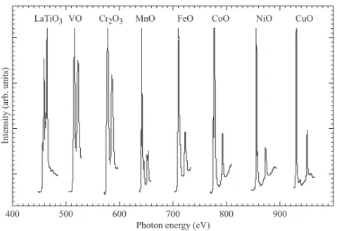
With the recognition that the local orbital occupation plays an important role in many of the transition metal compounds there is a need for experimental techniques that can measure the orbital occupation. This technique is soft x-ray absorption spectroscopy. For transition metal atoms one measures the local transition of a 2 p core electron into the 3 d valence shell. This type of spectroscopy has only developed into maturity over the last 20 years, both in terms of instrumentation as well as in terms of theoretical understanding of these spectra [18–20]. The pioneering work of Fink, Thole, Sawatzky and Fug- gle, who used electron energy loss spectroscopy on narrow band and impurity systems has been very important for the development of soft x-ray absorption spectroscopy. They recognized, that the observed multiplet structures can pro- vide an extremely detailed information about the local electronic structure of the ground and lower excited states of the system [21–23].

The 2 p core-electron excitation into the 3 d shell is dipole allowed. This has, first of all the advantage that good intensities are found. The locally dipole allowed transition has also the advantage of obeying the strict dipole selec- tion rules. This means that the intensity found for a given final-state depends strongly on the symmetry of the initial state. In most cases the dependence on the initial state symmetry is so large that one does not need to have good resolution in order to determine which of the possible states is realized as the ground-state. Within chapter 2 we will show many examples taken from the lit- erature of what can be measured with the use of x-ray absorption spectroscopy and how these dipole selection rules are active.

1.2 Interpretation of x-ray absorption spectros- copy

For the interpretation of 2 p x-ray absorption spectra cluster calculations are

an essential tool. At the moment cluster calculations are still one of the best

methods to describe both near ground-state properties and spectra of transi-

tion metal compounds. This might seem surprising while cluster calculations

are not ab-inito and the translational symmetry of the solid is not taken into

account. There are two reasons why cluster calculations are so powerful. The

first reason is that within cluster calculations the initial state and the final state

1.2 Interpretation of x-ray absorption spectroscopy 3

are treated on an equal footing. This results in calculated spectra that can be compared to experiments in great detail. This is in strong contrast to density functional methods or Hartree-Fock methods which produce density of states and not spectra. One should realize that a density of states is not a spectrum.

The second reason is that within cluster calculations the full electron-electron repulsion Hamiltonian can be included. The importance of full multiplet theory for the description of transition metal compounds will be stressed within the next section.

Part of the breakthrough in the understanding of 2 p x-ray absorption spec- troscopy on transition metal compounds was realized with the creation of good computation codes that can calculate the spectra of a cluster. Here the work done by Theo Thole [18, 21] and Arata Tanaka [24] must be mentioned who both wrote a program able to do cluster calculations and calculate the x-ray absorption spectra with all its multiplet structure up to great detail.

Initial state PES final state XAS final state

d ⁿ d ⁿ⁺¹ L d ^{n+2 2} L

∆

∆+U _dd

d ^n-1 d ⁿ L d ^{n+1 2} L d ^{n+2 3} L

∆-U _dd

∆

∆+U _dd

pd ⁿ⁺¹ p d ⁿ⁺² L p d ^{n+3 2} L

∆+U -U _{dd dp}

∆+2U _{dd dp} -U 2p-core level

PES final state

pd ⁿ p d ⁿ⁺¹ L p d ^{n+2 2} L p d ^{n+3 3} L

∆-U _dp

∆+U -U _{dd dp}

∆+2U _{dd dp} -U

Figure 1.1: On-site energies of the bare configurations for the initial state and different final states. ∆ is the energy it costs to hop with one electron from the oxygen band to the transition metal d shell. U is the repulsive Coulomb energy between two electrons in the 3 d shell ( U dd ) or between a 3 d electron and a 2 p core electron ( U dp ). L denotes the oxygen or ligand states and L ⁿ stands for n holes in the ligands. The holes in the p shell for the 2 p -core level PES final states and for the XAS final states are holes in the 2 p -core level of the 3 d transition metal ions. Scheme taken from J. Zaanen, G. A. Sawatzky and J. W.

Allen [6].

The cluster calculations are done within the configuration interaction scheme,

allowing for the inclusion of hybridization of the transition metal d orbitals with the oxygen p orbitals [25–27], denoted as the ligand orbitals ( L ). The on-site energies are parameterized with U and ∆ in the same way as done by J. Zaa- nen, G. A. Sawatzky and J. W. Allen [6]. In figure 1.1 we show the energy level diagram for the initial state and the final states of valence-band photo-electron spectroscopy, 2 p -core level photo-electron spectroscopy and 2 p -core level x-ray absorption spectroscopy. For the last two spectroscopies, the 2 p -core levels are core levels of the transition metal ions. For the initial state only the few lowest states are important. For the final state in principle all different configurations can be reached and are therefore important. The intensity of each final state does depend on the dipolar matrix elements between the initial state wave func- tion and the final state wave-function under consideration. In order to reproduce the measured x-ray absorption spectra one has to have the correct final state as well as the correct initial state within the cluster calculation. This means that detailed information concerning the initial-state can be obtained once the spectrum has been reproduced.

In figure 1.1 we only showed the on-site energies of the different configu- rations. The configurations will be split into different states. First of all the hybridization of different orbitals is not equal. For a transition metal in O h

symmetry the e g orbitals hybridize more with the oxygen orbitals then the t 2 g

orbitals. States with more holes in the e g shell will therefore be more covalent and have different energies than states where the e g orbitals are occupied. Sec- ond there will be a splitting due to the crystal field. Within mean-field theory this crystal field originates from the electric field made by the charges of the atoms that surround the atom under consideration. For transition metal oxides the oxygen atoms are charged negative and the electrons at the metal site do want to point away from the oxygen atom. Within O h symmetry this means that the t 2g orbitals are lowered with respect to the e g orbitals. Third there will be a splitting between the different states within one configuration due to the electron-electron repulsion. The importance of electron-electron repulsion and the effect of screening for 3 d elements will be discussed within the next section. Forth there are the spin-orbit coupling and magnetic interactions that split the different states within one configuration. Within a cluster calculation these interactions can be included and for many systems have to be included in order to reproduce the x-ray absorption spectra properly.

Besides cluster calculations there is an other way to deduce information from

x-ray absorption spectra. B. T. Thole, P. Carra et al. [28, 29] have derived sum-

rules that relate the total integrated intensity of polarized spectra to expectation

values of some operators of the initial state. These sum-rules are very powerful

due to there simplicity of use.

1.3 The importance of full multiplet theory 5

1.3 The importance of full multiplet theory

One might expect that within a solid the multiplet splitting due to electron- electron repulsion is largely screened. For the monopole part of the electron- electron repulsion this is indeed true. If one adds an extra charge to one atom within the solid the charges of the surrounding atoms (or other shells of the same atom) will change and thereby lower the total repulsion the added charge feels. This type of screening is also found experimentally. We define U av as the local average repulsion between two electrons. U av can be related to the Slater Integrals, F ⁰ , F ² and F ⁴ . The expression then becomes; U av = F ⁰ −

441 14 ( F ² + F ⁴ ). This U av is within a solid much smaller than the Hartree-Fock value found for a free ion. Take Co ²⁺ in CoO for example. The Hartree-Fock value of U av for the free ion is about 25 eV. The U av experimentally found is about 6.5 eV [24].

Surprisingly the multiplet splitting within a configuration in the solid is ex- perimentally found not to be reduced from the free ion multiplet splitting. E.

Antonides, E. C. Janse and G. A. Sawatzky [30] did Auger spectroscopy on Cu, Zn, Ga and Ge metal and found that the F ² and F ⁴ Slater integrals, the param- eters describing the multiplet splitting between states with the same number of electrons are in reasonable agreement with Hartree-Fock calculations on a free ion. This implies that only F ⁰ can be efficiently screened. These findings have been confirmed on many transition metal compounds [20, 26, 27, 31–34]. This absence of screening for the multiplet part of the electron-electron interaction can be understood if one realizes that the multiplet splitting is due to the differ- ent shape of the local electron cloud and\or due to different spin densities. Such differences are very difficult to screen by charges located externally. Moreover, there are also even states that have the same spin-resolved electron density ma- trix, d ^† mσ d m ⁰ σ ⁰ , but very different electron-electron repulsion interaction. Take a Ni ²⁺ ion for example. The ³ F M L =±3 ,M S =0 state, which belongs to the 21 fold degenerate ground-state, and the ¹ G M L =±3 ,M S =0 state have the same electron density matrix d ^† mσ d m ⁰ σ ⁰ but an energy difference of ¹² ₄₉ F ² + ₄₄₁ ¹⁰ F ⁴ . Within a mean-field approximation it is not possible to screen this splitting since these states have the same electron densities.

The full electron-electron interaction Hamiltonian is give by [31, 35, 36]:

H e − e = X

hmm ⁰ m ⁰⁰ m ⁰⁰⁰ σσ ⁰ i

U mm ⁰ m ⁰⁰ m ⁰⁰⁰ σσ ⁰ l ^† mσ l ^0† m ⁰ σ ⁰ l m ^{00 00} σ l ⁰⁰⁰ m ⁰⁰⁰ σ ⁰ (1.1)

with:

U mm ⁰ m ⁰⁰ m ⁰⁰⁰ σσ ⁰ = δ ( m + m ⁰ , m ⁰⁰ + m ⁰⁰⁰ ) X ∞

k=0

hlm|C _m−m ^k 00 |l ⁰⁰ m ⁰⁰ ihl ⁰⁰⁰ m ⁰⁰⁰ |C _m ^k 000 −m ⁰ |l ⁰ m ⁰ iR ^k ( ll ⁰ l ⁰⁰ l ⁰⁰⁰ )

R ^k ( ll ⁰ l ⁰⁰ l ⁰⁰⁰ ) = e ² Z _∞

0

Z _∞

0

r ^k <

r > ^k+1

R ⁿ l ( r 1 ) R ⁿ l ^{0 0} ( r 2 ) R ⁿ l ^{00 00} ( r 1 ) R ⁿ l ^{000 000} ( r 2 ) r ₁ ² r ₂ ² δr 1 δr 2

(1.2) With r < = Min( r 1 , r 2 ) and r > = Max( r 1 , r 2 ). This Hamiltonian describes a scattering event of two electrons. These two electrons have before scattering the quantum numbers m ⁰⁰ , m ⁰⁰⁰ , σ and σ ⁰ . After the scatter event they have the quan- tum numbers m, m ⁰ , σ and σ ⁰ . The scatter intensity is given by U mm ⁰ m ⁰⁰ m ⁰⁰⁰ σσ ⁰ . The angular dependence can be solved analytically and is expressed in integrals over spherical harmonics. The radial part can not be solved analytically and is expressed in terms of Slater integrals over the radial wave equation; R ^k ( ll ⁰ l ⁰⁰ l ⁰⁰⁰ ).

For two d electrons interacting with each other, the only important values of k are k = 0 , 2 or 4. For these k values the radial integrals are expressed as F ⁰ , F ² and F ⁴ .

Many calculations done on solids containing transition metal ions do not include the full electron-electron Hamiltonian, but make an approximation. The simplest approximation that one can make is to describe the electron-electron repulsion by two parameters U 0 and J H , in which U 0 is the repulsive Coulomb energy between each pair of electrons and J H is the attractive Hund’s rule exchange interaction between each pair of electrons with parallel spin. This leads to the following Hamiltonian:

H e ^Simple − e = U 0

X

h mm ⁰ σσ ⁰ i

l ^† mσ l ^0† m ⁰ σ ⁰ l mσ l ⁰ m ⁰ σ ⁰

−J H

X

hmm ⁰ σi

l ^† mσ l ^0† m ⁰ σ l mσ l ⁰ m ⁰ σ

(1.3)

This Hamiltonian is built up entirely by number operators n mσ = l ^† mσ l mσ , and is therefore diagonal in the basis vectors that span the full electron-electron Hamiltonian.

This extremely simple Hamiltonian leads for the Hund’s rule high-spin ground-

state to remarkably good results [38]. In table 1.1 we compare the total energy of

a d ⁿ configuration ( n = 0 ... 10) calculated using the full multiplet theory to that

calculated using the simple scheme. To facilitate the comparison, we have rewrit-

ten the Slater integrals, F ⁰ , F ² and F ⁴ in terms of U 0 = F ⁰ , J H = ₁₄ ¹ ( F ² + F ⁴ )

and C = ₁₄ ¹ ( ⁹ ₇ F ² − ⁵ ₇ F ⁴ ). We now see that the simple scheme is even exact

in half of the n cases and has an error of C for the other cases. Whereby the

Hartree-Fock value of C ranges from 0.5 eV for Ti ²⁺ to 0.8 eV for Cu ²⁺ .

1.3 The importance of full multiplet theory 7

Coulomb energy of Hund’s rule ground-state

Full Hamiltonian Simple Kanamori Kanamori mean field

d ⁰ 0 0 0 0 0

d ¹ 0 0 0 0 0

d ² F ⁰ - ₄₉ ⁸ F ² - ₄₄₁ ⁹ F ⁴ U ₀ - J _H -C U ₀ - J _H U’ - J U’ - J d ³ 3F ⁰ - ¹⁵ ₄₉ F ² - ₄₄₁ ⁷² F ⁴ 3U ₀ - 3J _H -C 3U ₀ - 3J _H 3U’ - 3J 3U’ - 3J d ⁴ 6F ⁰ - ²¹ ₄₉ F ² - ¹⁸⁹ ₄₄₁ F ⁴ 6U ₀ - 6J _H 6U ₀ - 6J _H 6U’ - 6J 6U’ - 6J d ⁵ 10F ⁰ - ³⁵ ₄₉ F ² - ³¹⁵ ₄₄₁ F ⁴ 10U ₀ -10J _H 10U ₀ -10J _H 10U’ -10J 10U’ -10J d ⁶ 15F ⁰ - ³⁵ ₄₉ F ² - ³¹⁵ ₄₄₁ F ⁴ 15U ₀ -10J _H 15U ₀ -10J _H 14U’+ U-10J 14U’+ U-10J d ⁷ 21F ⁰ - ⁴³ ₄₉ F ² - ³²⁴ ₄₄₁ F ⁴ 21U ₀ -11J _H -C 21U ₀ -11J _H 19U’+2U-11J 19U’+2U-11J d ⁸ 28F ⁰ - ⁵⁰ ₄₉ F ² - ³⁸⁷ ₄₄₁ F ⁴ 28U ₀ -13J _H -C 28U ₀ -13J _H 25U’+3U-13J 25U’+3U-13J d ⁹ 36F ⁰ - ⁵⁶ ₄₉ F ² - ⁵⁰⁴ ₄₄₁ F ⁴ 36U ₀ -16J _H 36U ₀ -16J _H 32U’+4U-16J 32U’+4U-16J d ¹⁰ 45F ⁰ - ⁷⁰ ₄₉ F ² - ⁶³⁰ ₄₄₁ F ⁴ 45U ₀ -20J _H 45U ₀ -20J _H 40U’+5U-20J 40U’+5U-20J

Table 1.1: Energy of the Hund’s rule ground-state of a d ⁿ electron configura- tion for different schemes. The relation between the Slater integrals F ⁰ , F ² and F ⁴ and the parameters U 0 , J H , C , U ⁰ , U , J , J ⁰ is: U 0 = F ⁰ , J H = ₁₄ ¹ ( F ² + F ⁴ ), C = ₁₄ ¹ ( ⁹ ₇ F ² − ⁵ ₇ F ⁴ ), U ⁰ = U − 2 J , J ⁰ = J , U = F ⁰ + ₄₉ ⁴ F ² + ₄₄₁ ³⁶ F ⁴ and J = ^2.5 ₄₉ F ² + ^22.5 ₄₄₁ F ⁴ [37, 38]. The center of each multiplet for the full Hamilto- nian is E av ( d ⁿ ) = ( F ⁰ − ₄₄₁ ¹⁴ ( F ² + F ⁴ )) ^{n ( n} ₂ ⁻¹⁾ .

Effective Coulomb interaction U ef f for Hund’s rule ground-state Full Hamiltonian Simple Kanamori Kanamori

mean field d ¹ F ⁰ - ₄₉ ⁸ F ² - ₄₄₁ ⁹ F ⁴ U ₀ - J H -C U ₀ - J H U’- J U’- J d ² F ⁰ + ₄₉ ¹ F ² - ₄₄₁ ⁵⁴ F ⁴ U ₀ - J _H +C U ₀ - J _H U’- J U’- J d ³ F ⁰ + ₄₉ ¹ F ² - ₄₄₁ ⁵⁴ F ⁴ U ₀ - J _H +C U ₀ - J _H U’- J U’- J d ⁴ F ⁰ - ₄₉ ⁸ F ² - ₄₄₁ ⁹ F ⁴ U ₀ - J H -C U ₀ - J H U’- J U’- J d ⁵ F ⁰ + ¹⁴ ₄₉ F ² + ¹²⁶ ₄₄₁ F ⁴ U ₀ +4J _H U ₀ +4J _H U+4J U+4J d ⁶ F ⁰ - ₄₉ ⁸ F ² - ₄₄₁ ⁹ F ⁴ U ₀ - J H -C U ₀ - J H U’- J U’- J d ⁷ F ⁰ + ₄₉ ¹ F ² - ₄₄₁ ⁵⁴ F ⁴ U ₀ - J _H +C U ₀ - J _H U’- J U’- J d ⁸ F ⁰ + ₄₉ ¹ F ² - ₄₄₁ ⁵⁴ F ⁴ U ₀ - J _H +C U ₀ - J _H U’- J U’- J d ⁹ F ⁰ - ₄₉ ⁸ F ² - ₄₄₁ ⁹ F ⁴ U ₀ - J H -C U ₀ - J H U’- J U’- J

Table 1.2: The effective Hubbard U between lowest Hund’s rule ground-state multiplets for different approximation schemes. The relation between the Slater integrals F ⁰ , F ² and F ⁴ and the parameters U 0 , J H , C , U ⁰ , U , J , J ⁰ is: U 0 = F ⁰ , J H = ₁₄ ¹ ( F ² + F ⁴ ), C = ₁₄ ¹ ( ⁹ ₇ F ² − ⁵ ₇ F ⁴ ), U ⁰ = U −2 J , J ⁰ = J , U = F ⁰ + ₄₉ ⁴ F ² +

441 36 F ⁴ and J = ^2.5 ₄₉ F ² + ^22.5 ₄₄₁ F ⁴ [37, 38]. The average U for the full Hamiltonian

is: U av = F ⁰ − ₄₄₁ ¹⁴ ( F ² + F ⁴ ).

This remarkable accuracy is important for the study of the conductivity gap in Mott-Hubbard insulators. The energy gap to move an electron from one site to another site far away is given by U :

U ( d ⁿ ) = E ( d ^{n −1} ) + E ( d ^{n +1} ) − 2 E ( d ⁿ ) (1.4) If multiplet effects are important, then there will be many different manners to move the electron. The gap is equal to the cheapest way to move one electron from one site to another site far away and thus given by the U = U ef f. , which involves the lowest multiplet states and not by U av , which refers to the the multiplet average energies. In table 1.2 we have listed U ef f for the various d ⁿ configurations ( n = 1 ... 9), having the high-spin Hund’s rule ground-state. We can see here that the correspondence between the simple scheme and the full- multiplet theory is very good. The deviation is not more than C ≈ 0 . 5 ... 0 . 8 eV, which is quite acceptable since the accuracy in the determination of U 0 by experiment or calculation is of the same order.

The shortcomings of the simple scheme do, however, show up dramatically when we have to consider the presence of states other than the Hund’s rule ground-state. In figure 1.2 we show the energy level diagram for the d ⁿ config- uration ( n = 2 ... 5), in spherical symmetry as an example. We can see that the multiplet splitting within the simple scheme is very different from that within the full multiplet theory. This first of all means that the simple scheme is com- pletely useless for calculating high energy excitations, like soft-x-ray absorption spectra. One truly needs the full multiplet theory to explain the many sharp structures observed in experiments [20, 26, 27, 30–34]. Not only for spectroscopy the simple scheme is inadequate, also for calculating ground-state properties, such as the magnetic susceptibility: the multiplicities are quite different. Within the simplified scheme only the magnetic angular spin momentum S z is a good quantum number, whereas in the full electron-electron repulsion Hamiltonian also the angular momenta of spin and orbital moment, S and L , are good quan- tum numbers. In other words the simple scheme brakes symmetry. It is almost needles to state that the simple scheme is by far to inaccurate to calculate, the relative stability of, for instance, the different spin-states within a partic- ular configuration. Figure 1.2 shows clearly that the energy levels in the two schemes differ by many electron volts.

In order to improve on the simple scheme, but still simplify the full electron-

electron Hamiltonian we will have a look at the simplification as proposed by

J. Kanamori. He proposed a simplification that tries to preserve the multiplet

character of the electron-electron interaction as much as possible. The approxi-

mation he made is that the electron-electron scattering events can be expressed

in terms that only depend on wether the scattered electrons are in the same

band (orbital) or in different bands (orbitals). The Hamilton found by these

1.3 The importance of full multiplet theory 9

Full multiplet Simple

scheme Kanamori scheme

3 P

S = 1 _z ⁺ 3 F

1 S

1 G

1 D S =0 _z

(21) (9) (9) (1)

(5)

(20) (25)

(30) (14) 10 (1)

8

6

4

2 12

Multiplet ener gy (eV)

d configuration ² d configuration ³

18

16

14

12

Multiplet ener gy (eV)

20

10

(10)

(14)

(10) (18)

(28) (28) (12)

(100)

(20) (40)

(70) (10)

S = _z ⁺ ₂ ³ S = _z ⁺ ₂ ¹

4 F 4 P 2 G ² H

2 P 2 D 2 F 2 D

Multiplet ener gy (eV) Multiplet ener gy (eV)

22 24 26 28 30 32 34 36

38 40 42 44 46 48 50 52 1 S

1 D

1 G

5 D

2 D 2 P

2 G

6 S S = 2 _z ⁺

S = 1 _z ⁺

S =0 _z S = _z ⁺ ₂ ³

S = _z ⁺ ₂ ⁵ S = _z ⁺ ₂ ¹

(6) (56) (40) (70) (70) (10)

(2) (200)

(50)

(6) (18) (6) (10)

(25) (105) (35) (30) (14) (1)

(25) (9) (5) (1)

(10) (100) (100)

Kanamori scheme mean-field

S=1 S=0 S=0

S = 1 _z ⁺ S =0 _z S =0 _z

(20) (20) (10)

S= ³ ₂ S= ¹ ₂ S= ¹ ₂

S = _z ⁺ ₂ ³ S = _z ⁺ ₂ ¹ S = _z ⁺ ₂ ¹

(20) (60) (40) Full multiplet Simple

scheme Kanamori

scheme Kanamori scheme mean-field

Full multiplet Simple

scheme Kanamori

scheme Kanamori scheme mean-field Full multiplet Simple

scheme Kanamori

scheme Kanamori scheme mean-field

d configuration ⁴ d configuration ⁵

3 P 3 F 1 F 1 D 1 S ₃ D 1 G

3 H 3 P 3 F ³ G 1 I

(21) (9) (7) (5)

(21)(9)

(33)

S = 2 _z ⁺ S = 1 _z ⁺ S = 1 _z ⁺ S =0 _z S =0 _z S =0 _z

(10) (40) (30) (60) (60) (10)

S=2 S=1 S=1 S=0 S=0 S=0

S = _z ⁺ ₂ ⁵ S = _z ⁺ ₂ ³ S = _z ⁺ ₂ ¹

³ ₂ S = _z ⁺ ₂ ¹ S = _z ⁺ ₂ ¹

4 G 4 P 4 D

4

F 2 S 2 D 2 F 2 G

2

H

F 2 D 2 I

S= ⁵ ₂ S= ³ ₂ S=

S= ¹ ₂ S= ¹ ₂ S= ¹ ₂

(2) (10) (20+40) (120) (60) (10)

(2) (14) (2)

(28)(14)

(26) (10)

(20) (12) (36)

Figure 1.2: Energy levels of a d ² , d ³ , d ⁴ and a d ⁵ configuration in spheri- cal symmetry, split due to electron-electron repulsion within the full electron- electron repulsion Hamiltonian, a simplified scheme, as explained in the text, the Kanamori scheme and the Kanamori scheme calculated in mean-field the- ory. The values taken for the Slater integrals are F ⁰ =5 eV, F ² =10 eV and F ⁴ =6.25 eV. On the left of each term we wrote the term name. On the right of each term we show the multiplicity in brackets. The energies for the d ⁶ , d ⁷ and d ⁸ configurations can be found by the equivalence of electrons and holes.

In spherical symmetry the d ⁿ configuration has the same multiplet splitting as

the d ¹⁰⁻ⁿ configuration, only shifted in total energy.

approximations is [39]:

H _e−e ^Kanamori = U X

m

l ^† _m↑ l ^† _m↓ l m ↑ l m ↓

+ U ⁰ X

m6=m ⁰

l ^† _m↑ l ^0† m ⁰ ↓ l m↑ l ⁰ m ⁰ ↓

+ U ⁰ X

m>m ⁰ σ

l mσ ^† l ^0† m ⁰ σ l mσ l ⁰ m ⁰ σ

+ J X

m>m ⁰ σ

l ^† mσ l ^0† m ⁰ σ l ⁰ m ⁰ σ l mσ

+ J X

m 6= m ⁰

l _m↑ ^† l ^0† m ⁰ ↓ l ⁰ m ⁰ ↑ l m↓

+ J ⁰ X

m 6= m ⁰

l ^† _m↑ l ^† _m↓ l ⁰ m ⁰ ↑ l ⁰ m ⁰ ↓

(1.5)

U is the parameter that describes the direct repulsion between two elec- trons in the same orbital; U = R R

φ ^∗ ( r 1 ) φ ^∗ ( r 2 ) _{| r} ^{e 2}

1 − r ₂ | φ ( r 1 ) φ ( r 2 ) δr 1 δr 2 . U ⁰ describes the direct repulsion between two electrons in different orbitals; U ⁰ = R R φ ^∗ ( r 1 ) φ ^0∗ ( r 2 ) _{| r} ^{e 2}

1 − r ₂ | φ ( r 1 ) φ ⁰ ( r 2 ) δr 1 δr 2 . It is assumed that this repulsion is equal between all different orbitals, φ and φ ⁰ . One can easily understand that this is not true. For example, the repulsion between the d xy and the d x ² − y ²

orbital is larger than between the d z ² and the d x ² − y ² orbital. The value of U ⁰ taken when we compare the Kanamori scheme with the full multiplet calculation is the average of the repulsion between all different orbitals [37]. The process where two electrons are interchanged is described by the exchange integral;

J = R R

φ ^∗ ( r 1 ) φ ^0∗ ( r 2 ) _{| r} ^{e 2}

1 − r ₂ | φ ⁰ ( r 1 ) φ ( r 2 ) δr 1 δr 2 . The process where two elec- trons residing in the same orbital scatter on each other and are transferred from one orbital into another is characterized by the integral; J ⁰ = R R

φ ^∗ ( r 1 ) φ ^∗ ( r 2 )

e ²

|r 1 −r 2 | φ ⁰ ( r 1 ) φ ⁰ ( r 2 ) δr 1 δr 2 .

In table 1.1 and 1.2 we show the energy of the lowest Hund’s rule multiplet and the effective U within the Kanamori scheme. Like in the case of the simple scheme, one find that the Kanamori scheme gives very similar and sometimes identical values as the full multiplet theory, as long as one limits oneself to the high-spin Hund’s rule ground-state.

The energetics of the excited states and the multiplicities of the states as

calculated using the Kanamori scheme differ nevertheless still quite apprecia-

bly from the full multiplet theory. Although, the spread of the multiplets is

now much improved as compared to that coming from the simple scheme, the

Kanamori multiplet structure still will not be of use to explain the high energy

soft-x-ray absorption data, which usually contain many very detailed and sharp

1.3 The importance of full multiplet theory 11

fine structures. Also, like in the case for the simple scheme, the Kanamori ap- proximation will be quite unreliable when one wants to calculate the relative energies of the different spin-states within a particular d ⁿ configuration.

Nevertheless, the Kanamori scheme is better than the simple scheme: (1) The spread of the multiplet splitting is much better reproduced; (2) The mul- tiplicity for the Hund’s rule ground-state is less wrong; within the Kanamori scheme all states with maximum S are degenerate, while in the single scheme it is only all states with maximum |S z | ; and (3) within the Kanamori scheme S is a good quantum number, whereas in the simple scheme it is not.

Sofar we have discussed approximations made in the scattering amplitude U mm ⁰ m ⁰⁰ m ⁰⁰⁰ σσ ⁰ σ ⁰⁰ σ ⁰⁰⁰ . There are however, more fundamental approximations made when calculating the electron-electron repulsion. Within the electron- electron repulsion Hamiltonian U mm ⁰ m ⁰⁰ m ⁰⁰⁰ σσ ⁰ σ ⁰⁰ σ ⁰⁰⁰ is multiplied by two creation and two annihilation operators, l ^† mσ l ^0† m ⁰ σ ⁰ l ⁰⁰ m ⁰⁰ σ l m ^{000 000} σ ⁰ . In order to calculate eigen- values of a particular state one has to evaluate the integral hl mσ ^† l ^0† m ⁰ σ ⁰ l ⁰⁰ m ⁰⁰ σ l ⁰⁰⁰ m ⁰⁰⁰ σ ⁰ i.

If one uses a mean-field approximation, the Hartree-Fock approximation or den- sity functional theory, this integral over four operators reduces to two integrals over two operators, hl ^† mσ l ⁰⁰ _m 00 σ ihl ^0† _m 0 σ ⁰ l ⁰⁰⁰ _m 000 σ ⁰ i . We will discuss the effect of this mean field approximation within the Kanamori scheme, as it shows very instruc- tive what happens.

Within mean-field theory the expectation values of the Kanamori Hamilto- nian reduce to:

hH _e−e ^Kanamori i = U X

m

hl _m ^† _↑ l m ↑ ihl ^† _{m ↓} l m ↓ i + U ⁰ X

m 6= m ⁰

hl ^† _m↑ l m ↑ ihl ^0† _m 0 ↓ l ⁰ m ⁰ ↓ i + U ⁰ X

m>m ⁰ σ

hl ^† mσ l mσ ihl ^0† m ⁰ σ l ⁰ m ⁰ σ i

−J X

m>m ⁰ σ

hl ^† _mσ l mσ ihl ^0† _m 0 σ l ⁰ m ⁰ σ i

(1.6)

The two terms, J P

m 6= m ⁰ l m ^† ↑ l ^0† m ⁰ ↓ l ⁰ m ⁰ ↑ l m ↓ and J ⁰ P

m 6= m ⁰ l m ^† ↑ l ^† m ↓ l ⁰ m ⁰ ↑ l ⁰ m ⁰ ↓ drop

since they are only non-zero between two wave-functions that differ by two sin-

gle electron wave functions from each other. We now see that the Kanamori

Hamiltonian within mean-field theory only depends on number operators and

therefore that it is diagonal within the basis vectors that span the full electron-

electron Hamiltonian. Within mean-field theory there are remarkable similar-

ities between the Kanamori scheme and the simple approximation we started

with. The Kanamori Hamiltonian can in mean-field approximation be described

by three parameters, U , U ⁰ and J , in which U is the repulsive Coulomb energy

between two electrons in the same orbital, with opposite spin, U ⁰ is the repulsive

Coulomb energy between two electrons in different orbitals and J is the attrac- tive Hund’s exchange interaction between each pair of electrons with parallel spin. The only difference with the simple scheme is that we introduced a U and U ⁰ that accounts for a difference between repulsion when two electrons are in the same orbital, or if they are in a different orbital.

In table 1.1 and 1.2 we show the energy of the lowest Hund’s rule multiplet and the effective U in the mean-field approximation of the Kanamori scheme. It should not be a surprise that these values are very similar to the full-multiplet theory. In fact the values are identical to the values found for the Kanamori scheme. So for the energy of the Hund’s rule ground-state it does not matter if one calculates the Kanamori scheme in mean-field theory or not. The mul- tiplicity of the ground-state and the energies of the excited state as calculated within the Kanamori scheme within mean-field approximation differ consider- ably from the Kanamori scheme as can be seen in figure 1.2. The spread of the multiplets is, like in the simple scheme, much smaller than in the full multiplet calculation. The multiplicity of the ground-state is incorrect and similar as in the simple scheme, only S z is a good quantum number and S is not.

The importance of the full electron-electron repulsion Hamiltonian should not be underestimated. From high energy spectroscopy it has been shown that the full electron-electron repulsion Hamiltonian has to be included to explain the spectra. This is also true for ground-state properties. For example there is a lively discussion about the spin-states of many of the cobaltates materials synthesized. A meaningful comparison of different multiplet terms can only be done if the electron-electron repulsion is correctly included. The differences of total energies between different spin states are often small and the differences between the full electron-electron repulsion Hamiltonian and the approximations shown here are quite large. Another example is CoO. There one finds an ordered orbital momentum that is quite large and experiment hints that it even might be larger than 1 µ B [40]. For a d ⁷ system with one hole in the t 2 g orbitals this is not so easy to understand as the maximum orbital momentum of a t 2 g orbital is 1 µ B . The only way to understand this large orbital momentum is by inclusion of the correct full electron-electron repulsion Hamiltonian. A detailed explanation of this effect can be found in chapter 6.

Finally, we would like to remind the reader again that there are different definitions of U and J around. The U as defined in the simple scheme is equal to F ⁰ , the J to ₁₄ ¹ ( F ² + F ⁴ ). The U in the Kanamori scheme is equal to F ⁰ + ₄₉ ⁴ F ² + ₄₄₁ ³⁶ F ⁴ and the J to ^2.5 ₄₉ F ² + ^22.5 ₄₄₁ F ⁴ . Within full multiplet theory U av

is equal to F ⁰ + ₄₄₁ ¹⁴ ( F ² + F ⁴ ). The effective U ef f. depends on the configuration

one looks at. Within this thesis when we talk about U we mean the U defined

within the full multiplet theory with respect to the multiplet average.

1.4 Scope 13

1.4 Scope

This thesis can be divided into three parts. Within the first part, ranging from chapter 2 to 4 we will discuss some properties of x-ray absorption spectroscopy and show how these spectra can be interpreted with the use of cluster calcula- tions and sum-rules. The second part, ranging from chapter 5 to chapter 7 will be about applications in thin-film research. In these chapters we will have a closer look on strain induced low symmetry crystal fields and orbital and spin magnetic moments. The third part, ranging from chapter 8 to 10, will deal with spin and orbital degrees of freedom in bulk transition metal compounds.

In chapter 2 an overview from literature is given of the different material properties, or operator values, one can measure with the use of x-ray absorption spectroscopy. With the use of cluster calculations and dipole selection rules it is shown why x-ray absorption spectroscopy is extremely sensitive to many of the initial state operator values we are interested in.

In chapter 3 some concepts of cluster calculations are given. This overview is by no means complete, as already many very good textbooks exist on this topic. We do not concentrate on simplifications one can make in diagonalizing the Hamiltonian, but assume this is done with the use of a PC and brute force.

In chapter 4 we discuss the sum-rules present in x-ray absorption spec- troscopy as derived by Thole and Carra et al. [28, 29]. These sum-rules have become very important in the interpretation of x-ray absorption spectroscopy due to their simplicity of use. In chapter 4 we will spent some time on how these sum-rules can be derived based on second quantization on the same line of thought as proposed by M. Altarelli [41].

In chapter 5 we present linear dichroism in the Ni L 2,3 x-ray absorption spec- tra of a monolayer NiO(001) on Ag(001) capped with MgO (001). The dichroic signal appears to be very similar to the magnetic linear dichroism observed for thicker antiferromagnetic NiO films. A detailed experimental and theoretical analysis reveals, however, that the dichroism is caused by crystal field effects.

We present a practical experimental method for identifying the independent magnetic and crystal field contributions to the linear dichroic signal in spectra of NiO films with arbitrary thickness and lattice strain.

In chapter 6 we first used XAS to study the properties of CoO bulk, as well

as thin films. We confirm that the Co ion in CoO has a free orbital momentum

in cubic symmetry. We confirm that spin-orbit coupling is very important for

understanding the properties of CoO and show that it is not reduced from the

Hartree-Fock value for a free Co ²⁺ ion. With the use of cluster calculations we

can get a full consistent understanding of the XAS spectra and the polarization

dependence of CoO. For CoO thin films we used XAS to show that we can

control the orbital momentum and spin direction with the application of strain

to thin CoO films. This finding opens up great opportunities for the use of

exchange-bias, where people put an antiferromagnet adjoined to a ferromagnet

in order to shift the magnetization hysteresis loop in one of the magnetic field directions [42, 43]. With the application of strain in the antiferromagnet one can chose if the system will be exchange-biased in the plane of the thin film, or perpendicular to the thin film surface. It also has great implications for the understanding of the exchange-bias phenomenon so far. The exchange-bias effect takes place at the interface between the ferromagnet and antiferromagnet [44, 45]. At the interface there will be strain in the antiferromagnet and one can not assume that the antiferromagnet has the same spin structure at the interface as it has in the bulk.

In chapter 7 we show how one can orientate spins in antiferromagnetic thin films with low magnetocrystalline anisotropy ( d ³ , d ⁵ and d ⁸ systems in O h sym- metry) via the exchange coupling to adjacent antiferromagnetic films with high magnetocrystalline anisotropy ( d ⁶ and d ⁷ systems in nearly O h symmetry). We have grown MnO thin films on CoO thin films with different predetermined spin orientation. With the use of Mn L 2 , 3 soft x-ray absorption spectroscopy we show that the Mn spin ’follows’ the Co spin direction.

In chapter 8 we study the spin-state problem within the cobaltates. Normally one is used to discuss the spin direction, or the magnetic spin angular momen- tum, S z . Within the cobaltates, d ⁶ compounds, there is however a discussion about the size of the spin, or the spin angular momentum, S ² = S ( S + 1). S ² can be 0, 2, or 6 (S=0,1,2), referred to as a low-spin state, an intermediate-spin state and a high-spin state. Within the literature there is a lot of confusion about the spin state as deduced from magnetic, neutron and x-ray diffraction measurements in the newly synthesized layered cobalt perovskits [46–70]. These measurements determine the size of the spin angular momentum ( S ² ) from the maximum size of the magnetic spin momentum S z . XAS is directly sensitive to the expectation value of S ² , the spin angular momentum. We carried out a test experiment using a relatively simple model compound, namely Sr ₂ CoO ₃ Cl, in which there are no spin state transitions present and in which there is only one kind of Co ³⁺ ion coordination [63, 64]. Important is that this coordina- tion is identical to the pyramidal CoO ₅ present in the heavily debated layered perovskites [46–62]. Using a spectroscopic tool, that is soft x-ray absorption spectroscopy (XAS), we demonstrate that pyramidal Co ³⁺ ions are not in the often claimed intermediate-spin state but unambiguously in a high-spin state.

This outcome suggests that the spin states and their temperature dependence in layered cobalt perovskites may be rather different in nature from those proposed in the recent literature.

In chapter 9 we study LaTiO ₃ . There has been a strong debate about the

role of orbital degrees of freedom within the titanates and in LaTiO ₃ especially

[13, 71–79]. With the use of spin resolved circular polarized photo electron

spectroscopy we confirmed that the orbital momentum in LaTiO ₃ is indeed

quenched [74]. With the use of XAS we show that this is due to a relative

1.4 Scope 15

large crystal field in the order of 120 to 300 meV. For a realistic description of materials one should not forget that there is a strong coupling between the orbitals and the lattice.

In chapter 10 we look at the metal-insulator transition in VO ₂ . With the use of XAS we show that the metal-insulator transition within this material is accompanied by a change in orbital occupation. The orbital occupation changes from almost isotropic in the metallic phase to the almost completely σ -polarized in the insulating phase, in close agreement with the two-site cluster model [80].

This very strong orbital polarization leads in fact to a change of the electronic structure of VO ₂ from a 3-dimensional to effectively a 1-dimensional system [81].

The V ions in the chain along the c-axis are then very susceptible to a Peierls

transition. In this respect, the MIT in VO ₂ can indeed be regarded as a Peierls

transition [82]. However, to achieve the required dramatic change of the orbital

occupation one also need the condition that strong electron correlations bring

this narrow band system close to the Mott regime [83]. The MIT in VO ₂ may

therefore be labelled as a ”collaborative” Mott-Peierls transition.

Chapter 2

X-ray absorption spectroscopy

X-ray absorption spectroscopy (XAS) is based on core-level absorption. This means that one makes excitations with light of high energy with respect to the chemical binding energies of the system. These excitations are dipole allowed and therefore do have good absorption cross sections. For 2 p elements like C,N and O one can make a 1 s to 2 p excitation, found in the 300 - 700 eV range. For the 3 d transition metals one can make a 2 p to 3 d excitation found in the 350 to 950 eV energy range. The 4 d transition metals have their 2 p to 4 d excitations at an energy from 2000 to 3500 eV. For the rare earth Lanthanides one can make a 3 d to 4 f excitation found in the 800 to 1700 eV energy range. These are the most useful excitations, but more excitations are possible. For the 3 d elements one could make excitations into the 4 p shell, from 1s, but these excitations do not probe directly the valence shell and are therefore less informative. In this thesis we will concentrate on the 3 d transition metals and excitations from the 2 p to 3 d shell therein. Historically this absorption edge is called the L edge.

The light source used to create light within this energy range is synchrotron

radiation. Synchrotron radiation of modern synchrotrons is bright enough to

do most XAS experiments wanted. Important is, however, to be able to scan

through the energy range of the spectrum in a fast and reproducible way. Mod-

ern beam-lines become more and more stable and have a very good accuracy

and reproducibility, necessary in many of the dichroic experiments done in this

thesis. Stability really becomes a big issue when one wants to compare spectra

taken at different temperatures. The spectra in this thesis have been taken at

the banding magnet Dragon beam-line at the NSRRC of Taiwan and the un-

dulator Dragon beam-line ID08 at the ESRF in Grenoble. Although banding

magnet beam-lines are less brilliant than undulator beam-lines, they are still a

good choice for absorption spectroscopy. This while not the brilliancy of the light source is the bottle neck in many experiments, but stability, scanning speed and reproducibility is more important. The absorption measurements at ID08 have been done with a fixed gap of the undulator.

LaTiO ₃ VO Cr O _{2 3} MnO FeO CoO NiO CuO

Intensity (arb. units)

400 500 600 700 800 900

Photon energy (eV)

Figure 2.1: 2p-Core level spectroscopy of different transition metal compounds.

Each element has its absorption edge at a different energy.

In figure 2.1 we show the XAS spectra for some selected 3 d transition metal oxides. The first thing one should notice is that each element has its absorption edge at a different energy. The reason for that is actually very simple. The more protons in the nucleus the more the core electrons are bound to the ion and the more energy it will cost to bring a core electron into the valence shell.

The fact that each element has its own energy for the core level absorption edge makes XAS very powerful. By selecting the energy of a specific element one will get information about the properties of only that element in the material. This allows one to do element specific measurements.

There are some features that all 2 p core level XAS spectra have in common.

In figure 2.2 we show the 2 p -XAS spectra of NiO. One can clearly see two sets of peaks, one around 850 eV, the other around 867 eV. The spectrum is split in two parts due to the 2 p -core level spin-orbit coupling. This energy is not small, because the 2 p electrons are close to the core and therefore should be treated relativistically. Historical the two different peak structures are called the L 2

edge and the L 3 edge. In figure 2.1 one can see that the splitting between the

L 3 and the L 2 edge is larger for the late transition metal compounds than for the

early transition metal compounds. The late transition metal atoms have more

2.1 One-electron theory 19

Figure 2.2: A general example of 2 p -XAS. One can clearly see the general features present. The L 2

and the L 3 edges and the corre- sponding continuum edge-jumps about 15 eV higher.

NiO 2p - XAS L ₃ edge

L ₂ edge L 3 continuum

edge jump

L ₂ continuum edge jump

Intensity (arb. units)

840 845 850 855 860 865 870 875 880 885 Photon energy (eV)

charge at the nucleus and therefore a tighter bound 2 p shell, which enlarges the 2 p spin-orbit coupling constant. In figure 2.2 one can also see that the intensity above 885 eV is larger than the intensity below 845 eV. This is called the edge- jump. The increase in overall spectral intensity, often called the background, takes largely place in two distinct small energy areas. In accordance to G.

van der Laan et al. [84], these have been labelled as the continuum edge-jump belonging to the L 2 and the L 3 edge. We will show below that the L 2 and the L 3 edges are excitons. The 2 p -core hole is bound to the additional 3 d electron whereas the continuum-edge jump is due to non-bonding final states.

2.1 One-electron theory

In order to understand why these features are present we start by describing

what one should expect if no electron-electron correlations were present. With-

out correlations materials and there spectra can very well be explained in an

one-electron picture. In figure 2.3 we show, on the left side a density of states

(DOS) for an arbitrary insulator, with a 3 d valence shell. Below the fermi en-

ergy the levels are occupied and above the fermi energy they are empty. We

also show the 2 p core level at deep energies. Other core levels, the 1 s , 2 s , 3 s ,

and 3 p are omitted for clarity. The 2 p core level is a delta function, since there

is no overlap between core levels of neighboring atoms, resulting in a flat band

and a delta function as DOS. It is important to notice that we drew two delta

functions for the 2 p core level. This is done on purpose while the 2 p core level

is split by spin-orbit coupling. Since we are talking about a core level the spin-

orbit coupling constant is not small, but it varies from 1.88 eV for K to 15.7 eV

WARNING: one electron picture does no work for correlated systems!

Optical Spectroscopy

0 PES

IPES

0

0

XAS L ₂

XAS L ₃

hν _a hν _b Unoccupied DOS

Fermi level

Occupied DOS

2p _3/2 2p _1/2 h ν a h ν b

3/2 ζ _2p

Figure 2.3: Interpretation of spectra within a one-electron theory. The shape of the spectra represents the band-structure.

for Zn. The 2 p shell has an orbital momentum of 1 and spin of ¹ ₂ . This results for a 2 p electron in a total angular momentum j = ¹ ₂ or j = ³ ₂ . There are 2 times as much 2 p orbitals with j = ³ ₂ than orbitals with j = ¹ ₂ . Therefore we drew one delta function twice as high as the other one. Excitations made from the 2p orbital with j = ¹ ₂ to the 3 d valence band are called the L 2 edge and excitations made from the 2 p orbital with j = ³ ₂ the L 3 edge.

In the middle left panel of figure 2.3 we drew the photo emission spectra (PES) and inverse photo emission spectra (IPES). Within a single electron the- ory these types of spectroscopy measure the occupied and unoccupied DOS respectively. For optical spectroscopy one makes excitations from the occupied DOS to the unoccupied DOS. This means the spectra measured is a convolu- tion of both, the occupied and the unoccupied DOS. There is a minimum energy required to make an excitation at all, the optical gap. This is the distance be- tween the highest occupied state to the lowest unoccupied state. In the right panel of figure 2.3 we show the XAS spectra expected in a single electron theory.

The principle of x-ray spectroscopy is similar to optical spectroscopy, we make

an excitation from the occupied core DOS to the unoccupied DOS. Again the

spectrum found is a convolution of the core DOS with the unoccupied valence

DOS. But in this case the 2 p core DOS consists of 2 delta peaks. Therefore the

2 p XAS consists of 2 times the unoccupied DOS shifted in energy by ³ ₂ times the

2 p core level spin orbit constant. Thereby one should notice that, since there

are 2 times as much 2 p core orbitals with j = ³ ₂ than with j = ¹ ₂ , there is a

difference in intensity of a factor of two between the L 2 and L 3 edge.