Variable selection for discrimination of more than two classes where data are sparse

Variable selection for discrimination of more than two classes where data are sparse

Gero Szepannek Claus Weihs

Lehrstuhl f¨ ur Computergest¨ utzte Statistik Fachbereich Statistik

Universit¨ at Dortmund

Abstract In classification, with an increasing number of variables, the required number of observations grows drastically. In this paper we present an approach to put into effect the maximal possible variable selection, by splitting a K class classification problem into pairwise problems. The principle makes use of the possibility that a variable that discriminates two classes will not necessarily do so for all such class pairs.

We further present the construction of a classification rule based on the pairwise solutions by the Pairwise Coupling algorithm according to Hastie and Tibshirani (1998). The suggested proceedure can be applied to any classification method.

Finally, situations with lack of data in multidimensional spaces are investigated on different simulated data sets to illustrate the problem and the possible gain.

The principle is compared to the classical approach of linear and quadratic discriminant analysis.

1 Motivation and idea

In most classification procedures, the number of unknown parameters grows more than linearly with dimension of the data. It may be desirable to apply a method of variable selection for a meaningful reduction of the set of used variables for the classification problem.

In this paper an idea is presented as to how to maximally reduce the number of used variables in the classification rule in a manner of partial variable selection.

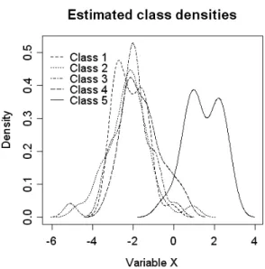
To motivate this, consider the example of 5 classes distributed in a variable as

it is shown in figure 1. It will be hardly possible to discriminate e.g. whether

an observation is of class 1 or 2. An object of class 5 instead will probably be

well recognized. The following matrix (rows and coloumns denoting the classes)

Figure 1: Example of 5 classes.

shows which pairs of classes can be discriminated in this variable:

C2 C3 C4 C5

C1 − − − +

C2 − − +

C3 − +

C4 +

(1)

We conclude that, since variables may serve for discrimination of some class pairs while at the same time not doing so for others, a class pair specific variable selection may be meaningful. Therefore we propose the following procedure:

1. Perform ”maximal” variable subset selection for all K(K −1)/2 class pairs.

2. Build K(K − 1)/2 class pairwise classification rules on possibly differing variable subspaces.

3. To classify a new object, perform K(K −1)/2 pairwise decisions, returning the same number of pairwise posterior probabilities.

The remaining question consists in building a classification rule out

of these K(K − 1)/2 pairwise classifiers.

2 Pairwise Coupling

2.1 Definitions

We now tackle the problem of finding posterior probabilities of a K-class clas- sification problem given the posterior probabilities for all K(K − 1)/2 pairwise comparisons. Let us start with some definitions.

Let p(x) = p = (p

, . . . , p

) be the vector of (unknown) posterior probabilities.

p depends on the specific realization x. For simplicity in notation we will omit x.

Assume the ”true” conditional probabilities of a pairwise classification problem to be given by

ρ

= P r(i|i ∪ j) = p

p

+ p

(2) Let r

denote the estimated posterior probabilities of the two-class problems.

The aim is now to find the vector of probabilities p

for a given set of values r

.

2.1.1 Example 1:

Given p = (0.7, 0.2, 0.1). The ρ

can be calculated according to equation 2 and can be presented in a matrix:

{ρ

} =





. 7/9 7/8

2/9 . 2/3

1/8 1/3 .



 (3)

The inverse problem does not necessarily have a proper solution, since there are only K − 1 free parameters but K(K − 1)/2 constraints.

2.1.2 Example 2:

Consider

{r

} =





. 0.9 0.4 0.1 . 0.7 0.6 0.3 .



 (4)

From Machine Learning, majority voting (”Which class wins most comparisons

?”) is a well known approach to solve such problems. But here, it will not lead to a result since any class wins exactly one comparison. Intuitively, class 1 may be preferable since it dominates the comparisons the most clearly.

2.2 Algorithm

In this section we present the Pairwise Coupling algorithm of Hastie and Tib-

shirani (1998) to find p for a given set of r

. They transform the problem into

an iterative optimization problem by introducing a criterion to measure the fit

between the observed r

and the ˆ ρ

, calculated from a possible solution ˆ p. To measure the fit they define the weighted Kullback-Leibler distance:

l(ˆ p) = X

i<j

n

r

∗ log r

ˆ ρ

+ (1 − r

) ∗ log

1 − r

1 − ρ ˆ

(5)

n

is the number of objects that fall into one of the classes i or j.

The best solution ˆ p of posterior probabilities is found as in Iterative Proportional Scaling (IPS) (for details on the IPS-method see e.g. Bishop, Fienberg and Holland, 1975). The algorithm consists of the following three steps:

1. Start with any ˆ p and calculate all ˆ µ

.

2. Repeat until convergence i = (1, 2, . . . , K, 1, . . .):

ˆ p

← p ˆ

∗

P

j6=i

n

r

P

j6=i

n

ρ ˆ

(6) renormalize ˆ p and calculate the new ˆ µ

3. Finally scale the solution to ˆ p ←

ipˆi

2.2.1 Motivation of the algorithm:

Hastie and Tibshirani (1998), show that l(p) increases at each step. For this reason, since it is bounded above by 0, the algorithm converges. The limit satis- fies P

i6=j

n

ρ

= P

i6=j

n

r

for every class i = 1, . . . , K if a solution p exists.

ˆ

p and ˆ ρ

are consistent.

Even if the choice of l(p) as optimization criterion is rather heuristic, it can be motivated in the following way: consider a random variable n

r

, being the rate of class i among the n

observations of class i and j. This random variable can be considered to be binomially distributed n

r

∼ B (n

, ρ

) with ”true”

(unknown) parameter ρ

. Since the same (training) data is used for all pairwise estimates r

, the r

are not independent, but if they were, l(p) of equation 5 would be equivalent to the log-likelihood of this model (see Bradley and Terry, 1952). Then, maximizing l(p) would correspond to maximum-likelihood estima- tion for ρ

.

Going back to example 2, we obtain ˆ p = (0.47, 0.25, 0.28), a result being consis- tent with the intuition that class 1 may be slightly preferable.

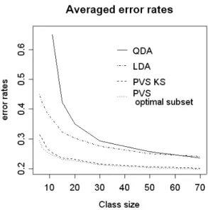
3 Validation of the principle

In this section, the suggested procedure of a pairwise variable selection combined with Pairwise Coupling [PVS] is compared to usual classification using linear and quadratic discriminant analysis [LDA, QDA].

Variable selection:

The method of variable selection in our implementation is a quite simple one.

We used class pair - wise Kolmogorov-Smirnov tests (see Hajek, 1969, pp.62–69) to check whether the distributions of two classes differ in a variable or not. For every class pair and every variable, the statistic

D = max

x

|F

(x) − F

(x)| (7)

is calculated, where the F

(x) are the empirical distributions of class k

, i = 1, 2. A variable is taken into a pairwise model if its p value strongly indicates differing densities. Of course, any other variable selection could be used instead.

3.1 A first example

Our first example is chosen according to the introductory example in section 1 to again illustrate the problem. Data are simulated in 9 classes and 10 variables.

Class i is distributed according to X ∼ N (2 ∗ 1.64 ∗ e

, I ) if i < 10 and X ∼ N(0, I), if i = 10. Here e

represents the standard basis vector, 0 is the 0 vector and I is the identity matrix.

This means, two classes k 6= l, k, l < 10 differ in their distributions in only 2 variables (k and l). Class 10 can be discriminated from any other class i only in variable i. By construction, no variable can be omitted. For that reason, variable selection will not remove any of the variables, using usual discriminant analysis. We computed the results for using LDA and QDA and compared it to the pairwise variable selection using LDA.

We computed simulations with varying (equal) class sizes in the training data to investigate the effect of sparse data. In the test data each class contains 50 objects. Error rates are averaged over 50 repetitive trials. The results are given in table 1.

QDA classification rules can only be build having enough data. Even at larger

Classes 1-9 Class 10

n LDA PVS(LDA) QDA LDA PVS(LDA) QDA

4 0.323 0.251 - 0.698 0.596 -

6 0.224 0.158 - 0.646 0.533 -

8 0.187 0.136 - 0.631 0.544 -

10 0.164 0.120 - 0.621 0.524 -

15 0.141 0.116 0.790 0.584 0.533 0.818

20 0.125 0.107 0.536 0.569 0.519 0.766

50 0.105 0.098 0.214 0.543 0.533 0.632

Table 1: Averaged error rates of LDA, QDA and PVS at varying class sizes

class sizes QDA error rates are very high. If there are few observations the PVS

approach shows strong advantages compared to usual LDA. For larger class sizes

the differences in the error rates of both methods seem to vanish.

3.2 Differing variances

We now extend the situation of the first example. In real life it may be possible that one is confronted with data where one of the classes is strongly concentrated in a specific variable. Of course, this class can be more easily identified by its realizations in this variable. Using LDA will fail to detect this by pooling all classes’ covariances.

We modelled this situation with data consisting of 10 classes and 10 variables.

Class i is distributed following X ∼ N (e

, Σ) with Σ being the identity except from (σ)

:= 0.1. An illustration of the phenomenon is given in figure 2.

Figure 2: Example of unequal variances and their pooled estimators.

Intuitively, QDA seems to be more appropriate in this situation. The results for varying training data sizes are shown in figure 3.

Astonishingly, here LDA still shows smaller error rates than QDA. For QDA, there does not seem to be enough data. Both methods can be largely improved by a class pairwise variable selection using QDA. The line with the smallest error rates is a reference line if the ”perfect” subset of variables would always be found. Surprisingly the KS-test yieds results that are very close to that line.

But note that such Variable selection will fail to detect situations of correlation between variables.

3.3 Waveform data

In order to obtain more general results we also wanted to apply the method to a common and well known classification problem. We chose the Waveform data introduced by Breiman et al. (1984).

The problem consists of simulated data of three classes and 21 variables. Three

waveforms over the variables (indexed by j) are given by: h

(j) = max(6 − |j −

Figure 3: Averaged error rates on test data.

11|, 0) , h

(j) = h

(j − 4) and h

(j) = h

(j + 4). h

(h

) is equal to h

but shifted to the left (right). For each object, its mean lies uniformly distributed between 2 of these waveforms over all 21 variables. The objects (depending on their class memberships) are given by

class 1 : X

= U h

(j) + (1 − U )h

(j) +

(8) class 2 : X

= U h

(j) + (1 − U )h

(j) +

(9) class 3 : X

= U h

(j) + (1 − U )h

(j) +

(10) where X

denotes variable j. U is an object specific random uniform number of the interval [0, 1] and

is an additional iid standard normal error. For class 2 and 3 the combination of waveforms changes.

The training data consists of 300 observations, each class having equal prior probabilities. The test data has 500 observations. We simulated 100 repetitions and averaged the error rates. It can be seen, that the results of both, linear

LDA PVS(LDA) QDA PVS(QDA) Bayes risk New Simulation 20.02 16.96 21.31 19.77

Breiman’s results 19.1 20.5 14.9

Table 2: Averaged error rates over 100 trials of Waveform data.

and quadratic discriminant analysis here can be improved by using the PVS-

approach.

3.4 Additional remarks

Situations, where a class pairwise variable selection will not lead to a further reduction of the variable space - compared to a K - class overall variable selection are not investigated yet.

In K-class LDA the posterior probabilities are found by normalizing the density estimations of the classes, given the observation x. Therefore, the conditional pairwise posterior probabilities for two classes using K-class LDA will be the same as in the pairwise approach, except from situations of different covariances of the classes. The covariance of PVS-LDA is pooled only by two instead of all K covariances. In the case of QDA there should not be any such difference between the K-class and pairwise classification rules since all covariances are estimated separately.

4 Summary

A principle is suggested to perform the maximal possible variable selection by splitting a K-class classification problem into K(K − 1)/2 two-class problems and an algorithm is presented to build a classification rule from the results using these methods. This principle can be applied to any classification method and any variable selection procedure.

The method is investigated on different simulated data sets using (linear and quadratic) discriminant analysis and the results are compared to their original results. Gain in classification error rate can be noticed, especially if the number of observations is not very large.

Additionally, the pairwise variable subset selection can give interpretational insight into which variables characterize the differences between two classes.

On the other hand, the computation time grows since there have to be built K(K − 1)/2 classification models. Also, the classification rule of each object has to be evaluated by the Pairwise Coupling algorithm.

Acknowledgment

This work has been supported by the Collaborative Research Center ’Reduc- tion of Complexity in Multivariate Data Structures’ (SFB 475) of the German Research Foundation (DFG).

References

BISHOP, Y., FIENBERG, S. and HOLLAND, P. (1975): Discrete multi- variate analysis, MIT Press, Cambridge.

BRADLEY, R. and TERRY, M. (1952): The rank analysis of incomplete

block designs, i. the method of paired comparisons, Bimometrics, 324–345.

BREIMAN, L. FRIEDMAN, J., OLSHEN, R. and STONE, C. (1984): Clas- sification and regression trees. Chapman & Hall, NY.

HAJEK, J. (1969): A course in nonparametric statistics. Holden Day, San Francisco.

HASTIE, T. and TIBSHIRANI, R. (1998): Classification by Pairwise Cou- pling. Annals of Statistics, 26(1), 451–471.

SCOTT, D. (1992): Multivariate Density Estimation Wiley, NY.