A simple variable selection technique for nonlinear models

A simple variable selection technique for nonlinear models

Gianluigi Rech, Timo Terasvirta and Rolf Tschernig Department of Economic Statistics,

Stockholm School of Economics, Box 6501, S-113 83, Stockholm, Sweden

Institut fur Statistik und Okonometrie, Humboldt-Universitat zu Berlin, Spandauer Str. 1, D-10178 Berlin, Germany

February 1, 1999 Abstract

Applying nonparametric variable selection criteria in nonlinear regression models generally requires a substantial computational e ort if the data set is large. In this paper we present a selection technique that is computation- ally much less demanding and performs well in comparison with methods currently available. It is based on a Taylor expansion of the nonlinear model around a given point in the sample space. Performing the selection only requires repeated least squares estimation of models that are linear in pa- rameters. The main limitation of the method is that the number of variables among which to select cannot be very large if the sample is small and an adequate Taylor expansion is of high order. Large samples can be handled without problems.

Keywords

: autoregression, nonlinear regression, nonlinear time series, nonparametric variable selection, time series modelling

AMS Classi cation Code:

62F07

Acknowledgments

: The work of the rst author has been nanced by the Tore Browaldh's Foundation. The second author acknowledges sup- port from the Swedish Council for Research in Humanities and Social Sci- ences. The research of the third author has been supported by the Deutsche Forschungsgemeinschaft via Sonderforschungsbereich 373 "Quanti kation und Simulation Okonomischer Prozesse" at Humboldt-Universitat zu Berlin.

1. Introduction

Selecting a subset of variables is a problem that has been extensively considered in linear models. The problem often occurs in connection with autoregressive models. In that case, the variables have an ordering, and sequential tests may be applied to choosing the maximum lag if it is nite. If one is also interested in nding the relevant lags, model selection criteria such as FPE (Akaike (1969)), AIC (Akaike (1974)), SBIC (Rissanen (1978) Schwarz (1978)) and many others may be applied.

The variable selection problem also occurs in nonlinear models. In some sit- uations, the functional form of the model may be unknown. The problem of nding the right subset of variables if it exists is then very important. This is because selecting too small a subset leads to misspecication whereas choosing too many variables aggravates the "curse of dimensionality". One way of solving the problem has been to use nonparametric methods based on local estimators.

For kernel estimators, Vieu (1995) and Yao and Tong (1994) considered variable selection based on cross-validation. On the other hand, Auestad and Tjstheim (1990) and Tjstheim and Auestad (1994) suggested nonparametric FPE criteria.

Their technique was further rened by Tschernig and Yang (1998) who, among other things, also showed the consistency of the FPE.

Even when the nonlinear model is parametric, a nonparametric variable se- lection technique could still be useful in many situations. For instance, if the researcher intends to t a neural network model to the data, then reducing the dimension of the observation vector before actually tting any model to data is advisable if possible. Nonparametric variable selection would save the researcher from the eort of estimating a possibly large number of neural network models with dierent combinations of variables before choosing the nal one.

In this paper we propose a simple variable selection procedure that instead of local estimation uses global parametric least squares estimation. It can never- theless be viewed as a nonparametric procedure as the number of parameters in the global regression is assumed to grow with the number of observations. This approach saves plenty of computational resources compared to nonparametric techniques based on local estimation. It can therefore be easily used even when the number of observations in the time series is large. The plan of the paper is as follows: Section 2 presents the idea and gives the theoretical motivation.

Section 3 outlines the model selection procedure. Section 4 reports results from a small-sample simulation study, and Section 5 concludes.

2. Asymptotic motivation

Consider the nonlinear model

y

t=

f

(^ut ) +

"

t

t

= 1

:::T

(2.1)

where ^ut = (

x

t¹

:::x

tp

z

t¹

:::z

tq)⁰ = (^x0_t

^z0_t)⁰ such that

E "

t ^{j F}t] = 0

where

Ft = ^fut

^ut^;1

:::

^g is the information set available at time

t

. Furthermore, we assume that

f

(^ut )

²

is a function of ^ut such that it is at least

k

times continuously dierentiable everywhere in the sample space^U =^{f u}t^jut^2Ug for all values of

²

:

Our problem is to nd the correct variables (elements of ^ut) for the model. Assume that those are

x

t¹

:::x

tp,

p

1, whereas the remaining elements of^ut are redundant.

We assume that the functional form of

f

is unknown even if the true function may be parametric. To nd the relevant variables, we start by linearizing

f

(^ut ).

This is done by expanding the function into a Taylor series around an arbitrary point ^u0_t ^{2 U}. After merging terms, the

k

-th order Taylor expansion can be written as:

f

(^xt

^zt

) =

⁰+^Xp

j⁼¹

_j

x

tj+^Xq

j⁼¹

_j

z

tj+^Xp

j¹⁼¹ p

X

j²⁼j¹

_j¹_j²

x

tj¹

x

tj²+^Xq

j¹⁼¹ q

X

j²⁼j¹

_j¹_j²

z

tj¹

z

tj²

+ ^Xp

j¹⁼¹ q

X

j²⁼¹

j¹j²

x

tj¹

z

tj² + ^Xp

j¹⁼¹ p

X

j²⁼j¹ p

X

j³⁼j²

_j¹_j²_j³

x

tj¹

x

tj²

x

tj³ +

:::

+ + ^Xq

j¹⁼¹ q

X

j²⁼j¹

q

X

j^k=j^{k ;1}

_j^1:::_j^k

z

tj¹

z

tj²

z

tj^{k ;1}

z

tj^k+

R

k(^ut) (2.2) where

q

k

(for notational reasons this is not a restriction),

R

k(^ut) is the remainder, and the

⁰s,

⁰s, and

's are parameters. Expansion (2

:

2) contains all possible combinations of

x

ti and

z

ti up to order

k

. The assumption that the true data-generating process is only a function of ^xt = (

x

t¹

:::x

tp)⁰ means that all the terms involving functions of elements of ^zt in (2

:

2) have zero coecients.

The remainder term will be a function of ^xt only:

R

k(^ut)

R

k(^xt)

⁸

t:

Thus the "true"

k

th-order expansion is

f

(^xt ) =

⁰+^Xp

j⁼¹

_j

x

tj+^Xp

j¹⁼¹ p

X

j²⁼j¹

_j¹_j²

x

tj¹

x

tj²+^Xp

j¹⁼¹ p

X

j²⁼j¹ p

X

j³⁼j²

_j¹_j²_j³

x

tj¹

x

tj²

x

tj³

+

:::

+

R

k(^xt)

:

(2.3)

Equation (2

:

2) may be written in matrix notation as

y=^X+^Zx+^R_k(^X

^Zx)+^" (2.4) where^Xis a

T

m

(

k

) matrix whose

t

^;th row involves products of elements of^xt

only,

t

= 1

:::T

and^Zxis a

T

n

(

k

) matrix whose

t

^;th row consists of elements involving at least one element of ^zt

t

= 1

:::T

. Setting ^W = ^{h X Zx i} and

=^;0

⁰⁰ and rewriting (2

:

3) yields

y=^W +^" (2.5)

where^" =^Rk(^X) +^" and^W is of full column rank.

We shall now make additional assumptions about (2

:

5).Assume that (White (1984), p. 119)

(i) (^wt

"

⁰_t)⁰ is a stationary ergodic sequence

(ii) (a)

E

^{f w0}

"

^{0 jF;}m^{g !} 0 in quadratic mean as

m

^{! 1} where ^Ft is the information set containing all information about^wt and ^"t up until

t

,

(b)

E

^j

"

t

w

ti ^j2

<

¹

i

= 1

:::m

(

k

) +

n

(

k

),

(c) VT =

var

T

^;1=2W0"is uniformly positive denite,

(d) 1

P

j⁼⁰

var

(

R

oij)¹⁼²

<

¹

i

= 1

:::m

(

k

) +

n

(

k

)

where

R

oij

=

E

(

w

⁰i

"

^{0 jF;}j)^;

E

w

⁰i

"

^0jF;(_j⁺¹⁾

i

= 1

:::m

(

k

) +

n

(

k

)

(iii) (a)

E

^j

w

ti^j2

<

¹

i

= 1

:::m

(

k

) +

n

(

k

),

(b) M=

E

^wt^w0t is positive denite.

Consider the case where

kT

^!1such that (

m

(

k

) +

n

(

k

))

=T

^!0 as

k

^!1. Furthermore,

R

k(^xt) ^!0 as

k

^!1

for any

k

1. The OLS estimator of in (2

:

5) has the form

b

=^;W0W;1W0y=+^;W0W;1W0(^R_k(^X) +^") (2.6) where =⁰

⁰⁰⁰

:

Note that the Taylor approximation becomes arbitrarily ac- curate as

k

^!1 thus

R

kt^!0 in probability for every

t

while (

m

(

k

)+

n

(

k

))

=T

^! 0

:

As

k

^!1

we have

plim _T^!1

k^!1

(m⁽k⁾⁺n⁽k⁾⁾=T^!0

(^b;) = plim _T!1

k^!1

(m⁽k⁾⁺n⁽k⁾⁾=T^!0

"

b

b

#

;

"

0n⁽k⁾

# !

= plim _T^!1

k^!1

(m⁽k⁾⁺n⁽k⁾⁾=T^!0

"

X 0

X

=T

^X0Zx

=T

Z

x 0

X

=T

^Zx0Zx

=T

#

;1

plim _T^!1

k^!1

(m⁽k⁾⁺n⁽k⁾⁾=T^!0

"

X 0

Rk(^X)

=T

Z

x 0

Rk(^X)

=T

#

+

"

X 0

"

=T

Z

x 0

"

=T

# !

=^M;11 plim _T^!1

k^!1

(m⁽k⁾⁺n⁽k⁾⁾=T^!0

"

X 0

"

=T

Z

x 0

"

=T

#

=⁰¹ (2.7)

where the subscript "¹" indicates an innite-dimensional matrix. Thus, asymp- totically, we are able to select the correct set of variables with probability

one. Furthermore, Theorem 5.16 (White (1984), p. 119) gives the asymptotic normality of ^p

T

(^{b ;}). The assumptions we need for these results are rather restrictive in the sense that all moments of^uthave to exist. However, if^uthas a multinormal distribution, say, then this assumption is satised. We shall discuss the practical implications of our asymptotic theory in Section 3.

The above theory is valid for ordinary regression models, but we would also like to select the appropriate lags in a nonlinear autoregressive model. We can expect our ideas to work in that framework only if we tighten the assumptions about the error structure of the model. Assume that the data-generating process is a nonlinear autoregressive model 2.1 where ^ut = (

y

t^;1

:::y

t^;p)⁰. It is not sucient to require that is

y

t is stationary. In addition, we also have to assume that at least 2

k

moments of

y

t exist if we want to use the

k

th order Taylor expansion. For asymptotic results similar to those in the previous section, we have to assume that all moments exist. This is the case if ^f

"

t^g is a sequence of zero-mean independent identically distributed stochastic variables such that all moments of their distribution are nite. This can be seen from the Volterra expansion of the autoregressive process for a denition see Priestley (1981), pp.

869-871.

3. The model selection procedure

The results of Section 2 show that, asymptotically, the combinations containing redundant variables will be discovered as their coecients that equal zero in the Taylor expansion are estimated consistently as are the other (nonzero) coecients.

The same may not be true for the univariate case, but we have argued that even the factors involving correct variables (lags) contribute more to the Taylor expansion than the other factors. This forms the starting-point of our model selection strategy. It can be described as follows. For a given sample size

T

, choose

k

, the order of the Taylor expansion. The asymptotic results suggest that the choice of

k

is important

k

has to be in the right proportion with respect to

T:

Then regress

y

t on all variables (product of original variables) in the Taylor expansion and compute the value of an appropriate model selection criterion. We use SBIC which is a relatively parsimonious criterion that Rissanen (1978) and Schwarz (1978) independently proposed: see, for example, Judge, Griths, Hill, Lutkepohl, and Lee (1984), pp. 862-874, or Terasvirta and Mellin (1986) for other alternatives. Next omit one regressor from the original model, regress

y

t on all products of variables remaining in the Taylor expansion and compute the value of SBIC. Repeat this by omitting each regressor in turn. Continue by simultaneously omitting two regressors from the original model. Proceed until the regression only consists of a Taylor expansion of a function with a single regressor. Leave this out as well to check for white noise. This amounts to estimating^Pp_i^=1+q;p+_i^q+1 = 2^p+q linear models by ordinary least squares. The combination of variables that yields the lowest value of SBIC is selected. If the number of observations is suciently

high and

k

is selected in an appropriate way, then one should be able to select the correct set of regressors with a high probability.

Sometimes the unknown function in (2

:

1) may be at least approximately lin- ear. Therefore it may be a good idea to begin the variable selection procedure by testing linearity. This can be done by testing the null hypothesis that the coe- cients of all the terms of order higher than one equal zero in the Taylor expansion (2

:

2). Terasvirta, Lin, and Granger (1993) arrived at this hypothesis when they derived a test of linearity against a single hidden layer feedforward articial neu- ral network model. If this hypothesis is not rejected, then the model selection simplies to variable selection in linear regression using subset regressions. This means saving computer time and making the selection procedure more ecient.

As before, a suitable model selection criterion such as SBIC may be applied to the problem. As we assume that the number of variables in

f

is xed, SBIC asymptotically yields the correct model with probability one, if the true model is linear.

In the next section we shall apply our procedure to demonstrate how its performs. We compare it with the FPE procedure by Tschernig and Yang (1998) that builds on the work by Tjstheim and Auestad (1994). That procedure was chosen since it is also consistent while requiring weaker moment assumptions, e.g. the function

f

() only needs to be dierentiable up to order four. This is achieved by using local estimation techniques. Instead of increasing the order of the Taylor expansion with increasing sample size as for the global estimator (2

:

2), the order of the Taylor expansion is xed while the expansion is estimated only locally. One thus estimates the function value

f

(^u) at^uby estimating a rst order expansion with observations lying in a neighbourhood of^u. Clearly, the smaller the neighbourhood determined by a so-called bandwidth parameter, the smaller the bias but the larger the estimation variance. With increasing sample size, the approximation error is reduced by decreasing the size of the neighbourhood instead of increasing the order

k

of the Taylor expansion.

The trade-o between bias and variance allows one to derive an asymptotically optimal bandwidth. Using recent results of Tschernig and Yang (1998), it can be estimated by plug-in methods. A corresponding estimate of

k

is beyond the scope of this paper. The nonparametric CAFPE proposed by Tschernig and Yang and used in the Monte Carlo analysis is given in equation (

A:

5) in the Appendix.

We shall only report results for univariate models. The results for multivariate models are similar to those for univariate ones and are therefore omitted.

4. A simulation study

To nd out how the selection procedure functions in practice, we conducted a simulation study. We simulated both nonlinear autoregressive models and models with exogenous regressors. The autoregressive data-generating processes (DGP) are dened as follows:

(i) Articial Neural Network model with two lags and a single hidden unit (^ANN1)

Y

t= 0

:

5 + 1

1 + exp^f;2(

Y

t^;1;3

Y

t^;2;0

:

05)^g +

"

t

"

t

N

0

10^;2 (4.1) (ii) Nonlinear Additive AR(2) process(^NLAR1)

Y

t=^;0

:

43^;

Y

_t^2;1

1 +

Y

_t^{2;1 + 0}

:

63^;(

Y

t^;2;0

:

5)³

1 + (

Y

t^;2;0

:

5)⁴ + 0

:

1

"

t

"

t

N

(0

1) (4.2)

(iii) Nonlinear Additive AR(4) process(^{NLAR1 14})

Y

t=^;0

:

43^;

Y

_t^2;1

1 +

Y

_t^{2;1 + 0}

:

63^;(

Y

t^;4;0

:

5)³

1 + (

Y

t^;4;0

:

5)⁴ + 0

:

1

"

t

"

t

N

(0

1) (4.3) (iv) Nonlinear AR(2) process (^NLAR4)

Y

t= 0

:

9 1

1 +

Y

_t^2;1+

Y

_t^{2;2 ;0}

:

7 + 0

:

1

"

t (4.4)

"

tTriangular density, positive for ^j

"

t^j

<

0

:

1^p6 (v) Logistic smooth transition autoregressive process (^LSTAR)

Y

t= 1

:

8

Y

t^;1;1

:

06

Y

t^;2+ (0

:

02^;0

:

90

Y

t^;1+ 0

:

795

Y

t^;2)

1 + exp^f;100(1

Y

t^;1;0

:

02)^g +

"

t

"

t

N

0

10^;2 (4.5) (vi) Periodic: (^SIN1)

Y

t= sin(

Y

t^;1) + sin(4

Y

t^;2)

2 +

"

t

"

t

N

0

10^;2 (4.6)

Simulating these processes did not indicate that any of them would be ex- plosive. The random numbers were generated by the random number generator in GAUSS, version 3.2. The rst 200 observations of each series were discarded.

Models (4

:

2), (4

:

3) and (4

:

6) are additive models (4

:

1)

(4

:

4)

(4

:

5) are not. This seems to make a dierence if we apply the nonparametric FPE procedure of Tsch- ernig and Yang (1998). The LSTAR model (4

:

5) is the same as that in Terasvirta (1994), p. 211 except for the error variance, which is greater. The periodic model (4

:

6) may be expected to be a problematic one as it is not well approximated by a combination of low-order polynomials of its variables. We also simulated models with exogenous regressors with the same functional form as the univariate ones, the lags being replaced by normally distributed exogenous regressors generated by a stationary rst-order vector autoregression. The results from both cases are rather similar, and we therefore only report those based on univariate models.

The remaining results are available from the authors upon request.

We used three sample sizes,

T

= 100

200

2000

in this study. To compare our procedure with the nonparametric approach, we also simulated the CAFPE procedure for the two smallest sample sizes. For

T

= 2000, the computing times for that technique turned out to be prohibitive. The idea with the smallest sample size is precisely to see how our procedure works when the available information set is not very large. The other two sample sizes are chosen (i) to show how much things improve compared to the smallest sample size and (ii) to demonstrate that the choice of

k

is important, that is, the ratio (

m

(

k

) +

n

(

k

))

=T

has to approach zero at a "right" rate as

T

increases.

Table 1 contains the results for

T

= 100

:

Most realizations from the nonlinear model (4

:

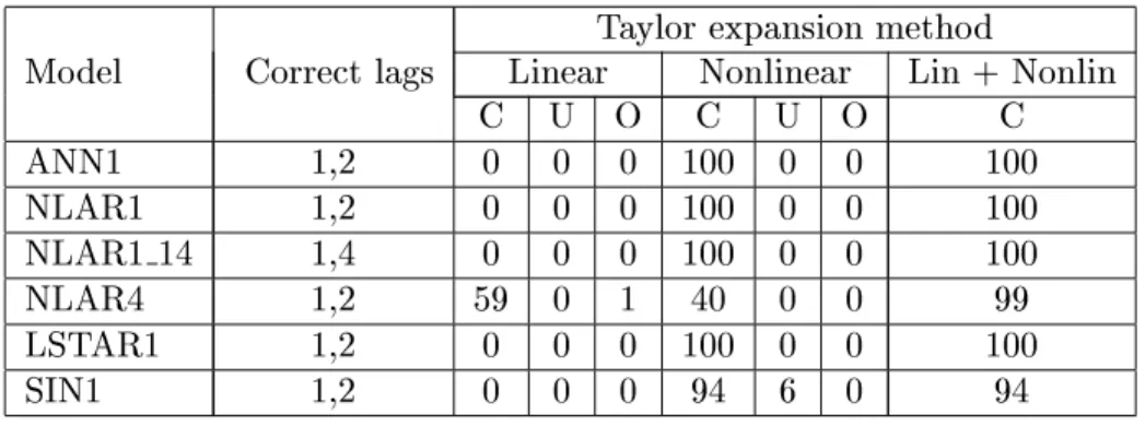
4) seem linear, and selecting the correct lags is more dicult than in other models. Note, however, that the ranking of the models in this respect may easily be changed by changing the error variance. Results also indicate that the nonparametric approach works better when the DGP is additive. In that case, CAFPE and our Taylor expansion strategy produce similar results. In other cases, our procedure compares quite favourably with the nonparametric one.

Tables 3 and 4 are based on 2000 observations. A comparison between them and Table 2 shows that the choice of

k

is important. If

k

= 3 as in Table 2 then, for the additive models, the performance of the procedure deteriorates compared to the smaller sample size. If

T

= 2000 but we choose a fth-order Taylor expansion, results are uniformly at least as good as for

T

= 200. An overall conclusion from this, admittedly limited, simulation experiment, is that the simple Taylor-expansion based model selection strategy works quite well. But this requires nding the right balance between the sample size, the number of variables under consideration, and the order of the Taylor expansion. Note in particular that for the periodic model (4

:

6), our technique performs adequately only for

T

= 2000 if, at the same time,

k

= 5. In small samples it is solidly beaten by the CAFPE.

The order of the autoregression

p

is restricted by the procedure because the number of regressors in the auxiliary regression grows exponentially with

p

and

k

. We can alleviate the problem as follows. If we disregard the cross terms in the Taylor expansion, we are able to reduce the number of regressors substantially.

This means implicitly assuming that the underlying model is additive. The lags selected this way normally encompass the set we would have selected with the complete expansion, if using that had been possible. Repeating the procedure with the complete Taylor expansion for the selected subset may then weed out the remaining redundant variables.

5. Conclusions

We have developed a variable selection technique that can be applied to nonlinear models and provided an asymptotic justication for it. Time series with a couple of hundred observations at most do not allow the set of variables to choose from to be large. On the other hand, the other techniques available for nonlinear model selection share this disadvantage. One of the main advantages of our technique is that it is simple and computationally feasible because it is based on ordinary least squares. It is applicable already in small samples and the computational burden remains tolerable even when the series are long. The standard subset selection procedure for linear models constitutes a special case of our technique.

In small samples the performance of our variable selection procedure compares favourably with currently available techniques based on nonparametric methods.

References

Akaike, H.(1969): \Fitting Autoregressive Models for Prediction," Ann. Inst.

Statist. Math., 21, 243{47.

(1974): \A New Look at the Statistical Model Identication," IEEE Trans. Autom. Control, AC-19, 716{23.

Auestad, B., ^and D. Tjstheim (1990): \Identication of Nonlinear Time Series: First Order Characterization and Order Determination," Biometrika, 77, 669{87.

Judge, G. G., W. E. Griffiths, R. C. Hill, H. Lutkepohl, ^and T.-C.

Lee(1984): The Theory and Practice of Econometrics. New York: Wiley.

Priestley, M.(1981): Spectral Analysis and Time Series. New York, Academic Press.

Rissanen, J.(1978): \Modeling by Shortest Data Description," Automatica, 14, 465{471.

Schwarz, G.(1978): \Estimating the Dimension of a Model," Ann. Statist., 6, 461{64.

Silverman, B. (1986): Density Estimation for Statistics and Data Analysis.

London: Chapman and Hall.

Terasvirta, T. (1994): \Specication, Estimation, and Evaluation of Smooth Transition Autoregressive Models," Journal of the American Statistical Asso- ciation, 89, 208{218.

Terasvirta, T., C.-F. J. Lin, ^andC. W. J. Granger(1993): \Power of the Neural Network Linearity Test," Journal of Time Series Analysis,¹⁴, 209{220.

Terasvirta, T., ^and I. Mellin (1986): \Model Selection Criteria and Model Selection Tests in Regression Models," Scandinavian Journal of Statistics, ¹³, 159{171.

Tjstheim, D.,^andB. Auestad(1994): \Nonparametric Identication of Non- linear Time Series: Selecting Signicant Lags," Journal of the American Sta- tistical Association,⁸⁹, 1410{1419.

Tschernig, R., ^and L. Yang (1998): \Nonparametric Lag Selection for Time Series," Discussion paper, Humboldt University Berlin.

Vieu, P.(1995): \Order Choice in Nonlinear Autoregressive Models," Statistics,

26, 307{328.

White, H.(1984): Asymptotic Theory for Econometricians. Orlando, FL: Aca- demic Press.

Yao, Q., ^and H. Tong (1994): \On Subset Selection in Non-Parametric Stochastic Regression," Statistica Sinica,⁴, 51{70.

Appendix

Denote by^wa (

m

1) subvector of^u,

m

p

+

q

. A local linear estimate

f

^b(^w

h

) of the function at^wusing the bandwidth

h

is given by the estimated constant ^

c

⁰ of a linear Taylor expansion tted locally around^w

fb

c

⁰

^bcg = arg min^f_c^0cgXT

t⁼¹

y

t^;

c

^0;(^wt^;w)^{0c 2}

K

h(^wt^;w) (

A:

1) where

K

() denotes a standard kernel function and

K

h(^wt^;w) =

h

^;mQ_mi⁼¹

K

((

w

ti^;

w

i)

=h

). The integrated mean squared error can then be estimated by

A

b(

h

) =

T

^;1XT

t⁼¹

n

y

t^;

f

^b(^wt

h

)^o2

w

(^ut) (

A:

2) where the integration is restricted to the domain of the weight function

w

() which is dened for the full vector ^u. Furthermore, dene the term

B

b(^b

h

B) =

T

^;1XT

t⁼¹

n

y

t^;

f

^b(^wt

^b

h

B)^o2

w

(^ut)

=

^b(^wt

^b

h

B) (

A:

3) where

^b() is a Gaussian kernel estimator of the density

using Silverman's (Silverman (1986)) rule-of-thumb bandwidth^b

h

B =

h

(

m

+ 2

T

^ ) and

h

(

kn

) =

^f4

=k

^g1=(k+2)

n

^;1=(k+2)

:

Moreover,

^b=^Q_mj^=1q

V ar

(^wj)^1=mdenotes the geometric mean of the standard deviation of the regressors.

The local linear estimate of the FPE is then given by

AFPE

=

A

^b(^b

h

opt) + 2

K

(0)^m

T

^;1b

h

^;_opt^m

B

^b(

h

^bB) (

A:

4) where the plug-in bandwidth is computed from

b

h

opt=ⁿ

m

^jj

K

^jj22m

B

^b(^b

h

B)

T

^;1

C

^b(^b

h

C)^;1

^;4_K ^o1=(m+4)

with^jj

K

^jj22 =^R

K

²(

u

)

du

,

²_K =^R

K

(

u

)

u

²

du

. Note that the second term in (

A:

4) serves as a penalty term to punish overtting.

The estimation of

C

involves second derivatives which are estimated with a local quadratic estimator that excludes all cross derivatives. It is a simplication of the partial local cubic estimator of Tschernig and Yang (1998). The bandwidth estimate^b

h

C is given by

h

(

m

+ 4

3

T

^b ).

Based on theoretical reasons and Monte Carlo evidence provided in Tschernig and Yang (1998), the authors suggest to use the corrected FPE

CAFPE

=

AFPE

ⁿ1 +

mT

^;4=(m+4)o (

A:

5) where the correction increases the probability of correct tting. One then chooses that variable vector ^w for which

AFPE

or

CAFPE

are minimized.

Table1. The number of correct choices among the rst⁵lags (^C), number of undertted models (^U fewer lags than in the correct model), number of overtted models (^O more lags than in the correct model) in 100 replications with

T

= 100 observations. Order of the Taylor expansion = 3.

Taylor expansion method CAFPE Model Correct lags Linear Nonlinear Lin + Nonlin

C U O C U O C C

ANN1 1,2 25 3 2 65 5 0 90 24

NLAR1 1,2 0 0 0 98 1 1 98 99

NLAR1 14 1,4 0 0 0 98 0 2 98 99

NLAR4 1,2 61 32 5 0 2 0 61 25

LSTAR1 1,2 57 5 0 31 7 0 88 46

SIN1 1,2 0 51 4 0 45 0 0 55

Table2. The number of correct choices among the rst 6 lags (^C), number of undertted models (^U fewer lags than in the correct model), number of overtted models (^O more lags than in the correct model) in 100 replications with

T

= 200 observations. Order of the Taylor expansion = 3.

Taylor expansion method CAFPE Model Correct lags Linear Nonlinear Lin + Nonlin

C U O C U O C C

ANN1 1,2 0 0 0 100 0 0 100 36

NLAR1 1,2 0 0 0 99 0 1 99 99

NLAR1 14 1,4 0 0 0 99 0 1 99 100

NLAR4 1,2 95 1 3 0 1 0 95 52

LSTAR1 1,2 13 0 0 86 1 0 99 43

SIN1 1,2 0 6 0 0 94 0 0 98

Table3. The number of correct choices among the rst 6 lags (^C), number of undertted models (^U fewer lags than in the correct model), number of overtted models (^O more lags than in the correct model) in 100 replications with

T

= 2000 observations. Order of the Taylor expansion = 3.

Taylor expansion method

Model Correct lags Linear Nonlinear Lin + Nonlin

C U O C U O C

ANN1 1,2 0 0 0 100 0 0 100

NLAR1 1,2 0 0 0 62 0 38 62

NLAR1 14 1,4 0 0 0 20 0 80 20

NLAR4 1,2 69 0 3 28 0 0 97

LSTAR1 1,2 0 0 0 100 0 0 100

SIN1 1,2 0 0 0 9 91 0 9

Table4. The number of correct choices among the rst 6 lags (^C), number of undertted models (^U fewer lags than in the correct model), number of overtted models (^O more lags than in the correct model) in 100 replications with

T

= 2000 observations. Order of the Taylor expansion =⁵.

Taylor expansion method

Model Correct lags Linear Nonlinear Lin + Nonlin

C U O C U O C

ANN1 1,2 0 0 0 100 0 0 100

NLAR1 1,2 0 0 0 100 0 0 100

NLAR1 14 1,4 0 0 0 100 0 0 100

NLAR4 1,2 59 0 1 40 0 0 99

LSTAR1 1,2 0 0 0 100 0 0 100

SIN1 1,2 0 0 0 94 6 0 94