A Factor
12Approximation Algorithm for a Class of Two-Stage Stochastic Mixed-Integer Programs
Nan Kong • Andrew J. Schaefer
Department of Industrial Engineering, University of Pittsburgh Pittsburgh, PA 15261, USA
nkong@ie.pitt.edu • schaefer@ie.pitt.edu
A Factor
12Approximation Algorithm for Two-Stage Stochastic Matching Problems
Nan Kong, Andrew J. Schaefer ∗
Department of Industrial Engineering, Univeristy of Pittsburgh, PA 15261, USA
Abstract
We introduce the two-stage stochastic maximum-weight matching problem and demonstrate that this problem isN P-complete. We give a factor 12 approximation algorithm and prove its correctness. We also provide a tight example to show the bound given by the algorithm is exactly 12. Computational results on some two-stage stochastic bipartite matching instances indicate that the performance of the approximation algorithm appears to be substantially better than its worst-case performance.
Keywords: Stochastic Programming; Approximation Algorithms; Matching; Combinatorial Optimization
1 Introduction
LetG = (V, E) be a graph, and let each edge e∈ E have an edge weight ce. The maximum- weight matching problem (Cook et al. 1998) is
max
X
e∈E
cexe X
e∈δ(v)
xe≤1, ∀v∈V; xe∈ {0,1}, ∀e∈E
. (1) It is well known that the maximum-weight matching problem is polynomially solvable (Edmonds 1965). Consider a stochastic programming extension of this problem as follows. Each edge has 2 weights, a first-stage weightce, and a discretely distributed second-stage weight ˜de. The first-stage decision x is to choose a matching in G. After the decision, a scenario of the second-stage edge weights is realized. That is, each edge weight is assigned to one of ther possible values d1e, . . . , dre with corresponding probabilitiesp1, . . . , pr. For each scenarios= 1, . . . , r, the second-stage decision ysis to choose a matching over those vertices unmatched by the first-stage matching. Without loss
∗Corresponding author. Email address: schaefer@ie.pitt.edu
of generality, the edge weights ce and dse for each scenario s= 1, . . . , r are nonnegative, since any edge with negative ce ordse won’t be chosen in any optimal solution. The goal is to maximize the total expected edge weight in these matchings. The stochastic programming extension of (1) can then be written as:
max X
e∈E
cexe + Xr
s=1
psX
e∈E
dseyse (2)
subject to
X
e∈δ(v)
xe+ X
e∈δ(v)
yes ≤ 1, ∀v ∈ V, s= 1, . . . , r xe ∈ {0,1}, yes ∈ {0,1}, ∀e ∈ E, s= 1, . . . , r.
For an introduction to stochastic programming, we refer to Kall and Wallace (1994), and Birge and Louveaux (1997). Interestingly, unlike the polynomially solvable deterministic maximum- weight matching problem, this stochastic programming extension isN P-complete, as will be shown in Section 2. Therefore, it is natural to develop approximation algorithms that finds solutions with a performance guarantee in a polynomial number of steps for the stochastic programming extension.
Hochbaum (1997) and Vazirani (2001) provided surveys of approximation algorithms. There have been very few studies of the computational complexity of stochastic programs and the applications of approximation algorithms to such problems. Dye et al. (2003) studied the computational complexity of the stochastic single-node service provision problem arises from an application of distributed processing in telecommunication networks. They showed the strongN P-completeness of the problem and presented several approximation algorithms.
The remainder of the paper is organized as follows. In Section 2, we show theN P-completeness of the stochastic matching problem. In Section 3, we present a factor 12 approximation algorithm and provide a class of instances for which the bound is tight. Section 4 provides computational results that show the performance of the approximation algorithm on a set of randomly generated two-stage stochastic bipartite matching instances.
2 The Complexity of Two-Stage Stochastic Matching
We state the two-stage stochastic matching problem formally.
INSTANCE: Graph G = (V, E), for each e ∈ E, first-stage edge weights ce and second-stage edge weightsdse fors= 1, . . . , r, and probabilityps for scenarios, a positive integer numberr, and a positive real number k.
QUESTION: Are there disjoint matchingsM0, M1, . . . , Mr in the graphGsuch thatM0∪Ms is a matching for s= 1, . . . , r and the total expected edge weight given by
X
e∈M0
ce + Xr
s=1
ps X
e∈Ms
dse (3)
is at least k?
Theorem 1 TWO-STAGE STOCHASTIC MATCHING is N P-complete.
Aboudi (1986) studied a similar problem, constrained matching, and demonstrated that it is also N P-complete with a somewhat similar proof.
Proof: TWO-STAGE STOCHASTIC MATCHING is clearly in N P. We assume that for all s, ps > 0, since any scenario with ps = 0 may be eliminated. We will use a reduction from CNF- SATISFIABILITY to establish the theorem. Let C be an expression in conjunctive normal form withρclauses: C = C1 ∧ C2 ∧ . . . ∧ Cρandq literalsx1, x2, . . . , xq. We assume thatxi and xi do not appear in the same clause, since each clause is a disjunction and thus any clause containing both xi andxi is always satisfied. We construct the graph Gas follows:
For each xi, create verticesvi, wi,andwi. For eachvi, construct edges (vi, wi) and (vi, wi). For each such edge e, letce = 1, and let dse= 0 for s= 1, . . . , ρ. For each Cs, create a vertex us. For i= 1, . . . , q, construct edges (wi, us) and (wi, us). For each edgee= (wi, us), letce = 0, and if xi is in Cs, let dse =ρ, otherwise, dse= 0. For each edgee= (wi, us), letce= 0, and if xi is inCs, let dse=ρ, otherwise, dse= 0. Definer ≡ρ and k≡ρ+q. Fors= 1, . . . , r, letps= 1r. Note that Gis a bipartite graph with bipartition (V +U, W), where V,U,W are the sets containing all vertices vi,us, and wi and wi, respectively.
We now claim that G contains matchings M0 ∪Ms for s = 1, . . . , r, and the total expected edge weight given in (3) is at leastk if and only if the expression C is satisfiable. To see this we demonstrate the correspondence between matchings with which the value of (3) is at leastkand a literal assignment which satisfies C.
Suppose that there exists a literal assignment that satisfies C. Construct the matchings M0, M1, . . . , Mr as follows.
1. For allxi, ifxi is True, add (vi, wi) to M0. 2. For allxi, ifxi is False, add (vi, wi) to M0.
3. For all clauses Cs, pick any literal that satisfies Cs. Ifxi is chosen, add (us, wi) to Ms. If xi is chosen, add (us, wi) toMs.
It is easy to check that M0∪Ms is a matching for s = 1, . . . , r, and the total expected edge weight isk.
Now let us suppose that there exist disjoint matchings M0, M1, . . . , Mr such that for s = 1, . . . , r, M0 ∪Ms is a matching and the total expected edge weight is at least k. Note that no more thanq edges withce >0 can be inM0, andce= 1 for all such edges. Also, note that for each s, no more than one edge withdse>0 can be inMs, anddse=ρ for this edge. Hence,Pe∈M0ce≤q and Pe∈Mspsdse≤1. The latter inequality implies that Prs=1Pe∈Mspsdse ≤ρ and thus the value of (3) is at mostq+ρ =k. Since the total expected edge weight is at leastk, it follows that M0 matches every vertex in V with a weight 1 edge and eachMs matches vertexus with a positively weighted edge.
Consider any literal in C, we construct the literal assignment as follows.
1. If (vi, wi) is inM0,xi isTrue.
2. If (vi, wi) is in M0,xi is False.
It is easy to check that this literal assignment satisfies C.
The above transformation is clearly polynomial, so we conclude thatTWO-STAGE STOCHAS- TIC MATCHING isN P-complete. 2
2.1 Example of the Reduction Consider the expression
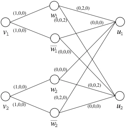
C={x1∨x2} ∧ {x1∨x2}. (4) There are two literals and two clauses, so r =ρ = 2, q = 2 andk= 4. Then Gis as in Figure 1 and the edge weights are as in Table 1. All edge weights are also labeled in Figure 1. The two scenarios are assigned with equal probability.
From Theorem 1, there exist disjoint matchings M0, M1 and M2 such that M0 ∪M1 and M0∪M2 are matchings and
X
e∈M0
ce + 1 2
X
e∈M1
d1e + 1 2
X
e∈M2
d2e ≥ 4
if and only if there exists a literal assignment satisfyingC.
Matchings M0 = {(v1, w1),(v2, w2)}, M1 = {(w1, u1)}, and M2 = {(w2, u2)} have a total expected weight of (1 + 1 + 2×12 + 2×12 = 4), and these matchings correspond to the assignment of literal x1 toFalse and literalx2 toFalsewhich satisfiesC. Note that M0∪M1 and M0∪M2 are matchings. An alternative is matchings M0 = {(v1, w1),(v2, w2)}, M1 = {(w1, u1)}, and M2 ={(w2, u2)}, which also have a total expected weight of 4, and correspond to the assignment of literalx1 toFalseand literalx2 toTrue which satisfiesC as well.
Table 1: Edge Weights of the Graph Constructed fromC e ce d1e d2e
(v1, w1) 1 0 0 (v1, w1) 1 0 0 (v2, w2) 1 0 0 (v2, w2) 1 0 0 (w1, u1) 0 2 0 (w1, u1) 0 0 0 (w2, u1) 0 0 0 (w2, u1) 0 2 0 (w1, u2) 0 0 2 (w1, u2) 0 0 0 (w2, u2) 0 0 2 (w2, u2) 0 0 0
3 A Factor
12Approximation Algorithm
Definition 1 A first-stage myopic solution is an optimal solution to:
(MYOPIC1) : max
X
e∈E
cexe X
e∈δ(v)
xe≤1, ∀v∈V; xe∈ {0,1}, ∀e∈E
. Definition 2 A second-stage myopic solution for scenario sis an optimal solution to:
(MYOPIC2) : max
X
e∈E
dseye X
e∈δ(v)
ye≤1, ∀v∈V; ye ∈ {0,1}, ∀e∈E
.
A first-(second-)stage myopic solution is the solution to a deterministic maximum-weight matching problem with the appropriate choice of objective.
The intuition behind our approximation algorithm is straightforward. We consider r+ 1 solu- tions: one first-stage myopic solution, and r second-stage myopic solutions for all scenarios. We compare two objective values: the objective value of the first-stage myopic solution, and the ex- pected objective value of the second-stage myopic solutions over all scenarios. Of these two values, the larger one gives the output of the approximation algorithm.
We state the algorithm formally:
Algorithm 1
INPUT: A two-stage stochastic maximum-weight matching problem.
Let x1 be a first-stage myopic solution, and letz1 =cx1.
For scenario s, Let y2s be a second-stage myopic solution, and let z2s=dsys2. Let zˆ= max{z1, Prs=1pszs2}.
OUTPUT: Ifzˆ=z1, then return(x1,0, . . . ,0)andz1; otherwise, return(0, y21, . . . , y2r)andPrs=1psz2s. Theorem 2 Algorithm 1 is an approximation algorithm with performance guarantee 12 for the two-stage stochastic maximum-weight matching problem given in (2).
Proof: Solutions (x1,0, . . . ,0) and (0, y12, . . . , yr2) are clearly feasible to (2). Letx∗ = (x0, y01, . . . , yr0) and z∗ be an optimal solution and the optimal objective value to (2), respectively. Since solution x0 is feasible to (MYOPIC1),
ˆ
z≥z1 ≥cx0. (5)
Since solution ys0 is feasible to (MYOPIC2) for scenario s,s= 1, . . . , r, ˆ
z≥ Xr
s=1
psz2s≥ Xr
s=1
psdsys0. (6)
Summing up inequalities (5) and (6) yields 2ˆz ≥ cx0 +Prs=1psdsys0 = z∗, and thus the result follows. 2
Since both (MYOPIC1) and (MYOPIC2) are polynomially solvable, Algorithm 1 runs in poly- nomial time.
3.1 A Tight Example for Algorithm 1
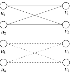
We give a tight example of two-stage stochastic bipartite matching. The problem is defined on the graph G= (V, E) as in Figure 2 and its objective function is given as in (2).
Let G be a bipartite graph with bipartition V = (S, T) where |S| = |T| and furthermore let S = (S1, S2) with |S1|=|S2| and letT = (T1, T2) with |T1|=|T2|. Let l be any positive integer.
For all edges e= (u, v) with u∈ S1 and v ∈ T1, let ce = l. For all other edges connecting S and T, letce = 0. For any scenarios,s= 1, . . . , r, for all edges e= (u, v) withu ∈S2 and v ∈T2, let dse = l; for all other edges connecting S and T, let dse = 0. Figure 2 illustrates such an instance with|S|=|T|= 4.
The first-stage myopic solution is given by choosing any complete matching from S1 to T1, together with any matching from S2 to T2. Hence, the output of Algorithm 1 is to use the first- stage myopic solution in the first stage and to choose no edges in the second stage. This output gives the total expected edge weightl·|V4|. For any scenario, the second-stage myopic solution is given by choosing any complete matching from S2 to T2, together with any matching from S1 to T1. Hence, the output of Algorithm 1 is to choose no edges in the first stage and to use the sth second-stage myopic solution in the second stage if scenarios s is realized. This output gives the total expected edge weightl·|V4|. The maximum of these two solutions isl·|V4|, so the approximation algorithm gives a solution of l·|V4| .
The optimal solution to the two-stage stochastic bipartite matching problem is to choose any complete matching from S1 to T1 as the first-stage decision, and for each scenario, choose any complete matching fromS2 toT2 as the second-stage decision. The first-stage matching gives edge weightl·|V4|, and the expected second-stage edge weight isl·|V4|, so the total expected edge weight isl·|V2|. Thus the approximation algorithm returns a solution whose total expected edge weight is exactly 12 of the optimal objective value.
4 Computational Results
We tested our approximation algorithm on a set of randomly generated two-stage stochastic bipartite matching instances with 10 vertices in each side of the bipartition and 100 scenarios. In our computational experiments, we used CPLEX 7.0 to find the solutions to (MYOPIC1) and (MY- OPIC2). To check the performance of our approximation algorithm, we also solved the stochastic programming formulation directly using the L-shaped method (Van Slyke and Wets 1969), a variant
of Benders’ decomposition (Benders 1962) and a standard technique for exactly solving two-stage stochastic linear programs. For some large instances, the L-shaped method tended to be very time-consuming, so we imposed a one-hour CPU time limit on it and obtained the solution of the restricted master problem, which is an upper bound on the exact solution.
In all test instances, the first-stage and second-stage edge weights were normally distributed. All scenarios were realized with equal probability. We tested four groups of instance classes, in each of which only one of the four distribution parameters (mean and standard deviation of the first-stage and second-stage edge weights) was varied and other three were fixed. For example, in group 1, we varied the mean of the first-stage edge weights from 5 to 25. We generated 100 instances for each instance class and reported the average CPU time. Table 2 presents the characteristics and computational results of these instance classes. Our computational experiments indicate that the CPU time of the approximation algorithm is insensitive to the distribution parameter settings. On the other hand, when the first-stage and second-stage edge weights are generated from the same or similar distributions, the L-shaped method is relatively less efficient due to the symmetry between the edge weights in the two stages. We also report the average ratio of the approximation solution to the exact solution in the table. When the first-stage and second-stage edge weights are generated from the same or similar distributions, this ratio tends to be the lowest by the same reason.
We then considered some large stochastic bipartite instances with 500 vertices in each side of the bipartition and 10 scenarios. Table 3 presents the characteristics and computational results of these instances. Each instance class consists of 10 instances. As above, each random parameter was generated according to a normal distribution and each scenario was assigned with equal probability.
In the table, we also report the average ratio of the approximate solution to the exact solution or its upper bound if the L-shaped method did not terminate within one hour.
5 Conclusions
As we have shown in this paper, the stochastic programming extension of a polynomially solvable combinatorial optimization problem may become N P-complete. However, the line between easy and hard stochastic combinatorial optimization problems has yet to be fully explored. Meanwhile, given difficulty of solving stochastic programs, particularly stochastic integer programs, developing approximation algorithms for such problems is a promising direction for future research.
Table 2: Characteristics and Computational Results of Small Instances
Average Average
Group Instance Average Average # of L-shaped Performance
1st stage 2nd stage Approx. CPU L-shaped CPU Iterations Ratio
∼N(5,152) ∼N(10,152) 0.08 0.71 13.39 0.976
∼N(10,152) ∼N(10,152) 0.08 1.88 25.35 0.958
1 ∼N(15,152) ∼N(10,152) 0.08 2.25 23.70 0.984
∼N(20,152) ∼N(10,152) 0.08 0.41 9.05 0.998
∼N(25,152) ∼N(10,152) 0.08 0.14 4.79 1.000
∼N(10,52) ∼N(10,152) 0.08 0.10 3.01 1.000
∼N(10,102) ∼N(10,152) 0.08 0.34 7.20 0.997
2 ∼N(10,152) ∼N(10,152) 0.08 1.88 25.35 0.958
∼N(10,202) ∼N(10,152) 0.08 1.21 18.93 0.966
∼N(10,252) ∼N(10,152) 0.08 0.53 11.54 0.978
∼N(10,152) ∼N(5,152) 0.08 1.81 21.97 0.980
∼N(10,152) ∼N(10,152) 0.08 1.88 25.35 0.958
3 ∼N(10,152) ∼N(15,152) 0.08 0.79 14.02 0.980
∼N(10,152) ∼N(20,152) 0.08 0.32 7.20 0.994
∼N(10,152) ∼N(25,152) 0.08 0.15 4.11 0.998
∼N(10,152) ∼N(10,52) 0.08 0.16 5.74 0.989
∼N(10,152) ∼N(10,102) 0.08 0.82 15.20 0.976
4 ∼N(10,152) ∼N(10,152) 0.08 1.88 25.35 0.958
∼N(10,152) ∼N(10,202) 0.09 0.97 12.66 0.991
∼N(10,152) ∼N(10,252) 0.09 0.19 4.86 0.999
Table 3: Characteristics and Computational Results of Larger Instances
Average Average
Instance Weights Average Average # of L-shaped Performance
Class First-stage Second-stage Approx. CPU L-shaped CPU Iterations Ratio
1 ∼N(10,152) ∼ N(10,152) 160.4 ≥3600 ≥ 3 0.954
2 ∼N(10,152) ∼ N(10,202) 144.9 ≥3600 ≥ 3 0.998
3 ∼N(10,152) ∼ N(10,302) 131.8 197.0 2 1.000
4 ∼N(15,152) ∼ N(10,152) 161.3 ≥3600 ≥ 3 0.986
5 ∼N(20,152) ∼ N(10,152) 159.7 ≥3600 ≥ 3 0.997
6 ∼N(20,152) ∼ N(10,302) 132.3 191.4 2 1.000
Acknowledgments
This research was partially supported by National Science Foundation grant DMI-0217190 and a grant from the University of Pittsburgh Central Research Development Fund.
Reference
Aboudi, R., 1986. A Constrained matching program: A polyhedral approach, Ph.D. Thesis, Cornell University, Ithaca, NY.
Benders, J.F., 1962. Partitioning procedures for solving mixed variables programming problems, Numerische Mathematics 4 238–252.
Birge, J.R., Louveaux, F.V., 1997. Introduction to Stochastic Programming, Springer, New York, NY.
Cook, W.J., Cunningham, W.H., Pulleyblank, W.R., Schrijver, A., 1998. Combinatorial Optimiza- tion, John Wiley and Sons, New York, NY.
Dye, S., Stougie, L., Tomasgard, A., 2003. Approximation algorithm and relaxations for a service provision problem on a telecommunication network, Discrete Applied Mathematics 129(1) 63–
81.
Edmonds, J., 1965. Maximum matching and a polyhedron with 0-1 vertices, Journal of Research of the National Bureau of Standards 69B 125–130.
Hochbaum, D.S., 1997. Approximation Algorithms for NP-hard Problems, PWS Publishing Com- pany, Boston, MA.
Kall P., Wallace, S.W., 1994. Stochastic Programming, John Wiley and Sons, Chichester, UK.
Van Slyke, R., Wets, R.J.-B., 1969. L-shaped linear programs with applications to optimal control and stochastic programming, SIAM Journal on Applied Mathematics 17 638–663.
Vazirani, V., 2001. Approximation Algorithms, Springer-Verlag, New York, NY.
u
1w
1w
2w
2w
1v
1v
2(1,0,0)
(1,0,0)
(0,0,2)
(0,2,0)
(0,0,0)
(0,0,0)
(0,0,0)
(0,0,2)
(0,0,0) (0,2,0)
(1,0,0)
(1,0,0)
u
2Figure 1: Example of the graphGconstructed from the expressionCgiven in (4). The edge weights are represented by (ce, d1e, . . . , dre).
u
1v
1u
2v
2u
3v
3u
4v
4Figure 2: Example on the complete bipartite graphGwhen the bound is tight. Edges with presence have positive edge weights. Solid edges are weightedlin the 1ststage and dashed edges are weighted l in the 2nd stage. All other edges have zero weight in both stages. S1 ={u1, u2},S2 ={u3, u4}, T1={v1, v2},T2={v3, v4}.