Phonons and crystal-field
excitations in highly correlated materials probed by optical
spectroscopy
Inaugural - Dissertation zur
Erlangung des Doktorgrades
der Mathematisch-Naturwissenschaftlichen Fakult¨ at der Universit¨ at zu K¨ oln
vorgelegt von
Thomas Andr´e David M¨oller
aus K¨ oln
K¨ oln, im Februar 2009
Vorsitzender
der Pr¨ ufungskommission: Prof. Dr. L. Bohat´ y
Tag der m¨ undlichen Pr¨ ufung: 28. April 2009
F¨ ur meine Frau Melanie,
meine Eltern,
meine Familie.
Contents
1 Introduction 1
2 Calculating the Electronic Structure of a Crystal 5
2.1 The Hartree-Fock Calculation . . . . 8
2.1.1 Hartree-Fock Theory and Slater Determinants . . . . 8
2.1.2 Self-Consistent Field Technique . . . . 9
2.1.3 Radial Schr¨ odinger Equation . . . . 11
2.2 Configuration-Interaction Method . . . . 15
2.2.1 Configuration Interaction . . . . 15
2.2.2 Correlation Energy . . . . 16
2.2.3 Truncated Configuration Interaction . . . . 16
2.3 Coupled Antisymmetrized Basis Functions . . . . 18
2.3.1 Coefficients of Fractional Parentage . . . . 18
2.3.2 Basis Functions within the Russell-Saunders-coupling scheme . . 19
2.3.3 One- and Two-Electron Operators . . . . 20
2.4 Racah-Wigner Algebra . . . . 26
2.4.1 Irreducible Tensor Operator . . . . 26
2.4.2 Wigner-Eckart Theorem . . . . 27
2.4.3 Matrix Elements of Tensor Operators . . . . 28
2.4.4 Unit Double Tensor Operator . . . . 29
2.5 Coulomb Interaction . . . . 31
2.5.1 Coulomb Operator . . . . 31
2.5.2 Slater Integrals . . . . 32
2.5.3 Direct Interaction between Equivalent Electrons . . . . 33
2.5.4 Direct Interaction between Non-Equivalent Electrons . . . . 34
2.5.5 Exchange Interaction between Non-Equivalent Electrons . . . . 36
2.5.6 Direct and Exchange Interaction between Non-Equivalent Elec- trons . . . . 37
2.6 Crystal Field Splitting . . . . 39
2.6.1 Crystal-Field Theory and Ewald Sum Formulation . . . . 39
2.6.2 Matrix Elements of the Crystal-Field Operator . . . . 40
2.7 Spin-Orbit Interaction . . . . 42
2.8 Hybridization and Tight-Binding Approximation . . . . 45
2.8.1 Linear Combination of Atomic Orbitals (LCAO) . . . . 45
2.8.2 Hopping Integrals . . . . 46
2.8.3 Slater-Koster Approximation . . . . 47
2.8.4 Sharma’s Method . . . . 48
2.8.5 Harrison’s Rules . . . . 49
2.8.6 Sobel’man’s Parentage-Scheme Approximation . . . . 50
2.8.7 Racah-Wigner expression for the tight-binding operator . . . . . 52
2.9 Exchange Interactions . . . . 56
2.10 External Fields . . . . 58
2.10.1 Stark Effect . . . . 58
2.10.2 Zeeman Splitting . . . . 60
2.11 Observable . . . . 63
2.11.1 Response Functions and Optical Conductivity . . . . 63
2.11.2 Magnetic Susceptibility . . . . 66
2.11.3 Phonons . . . . 67
2.12 Numerical calculation . . . . 70
2.12.1 Lanczos algorithm . . . . 70
2.12.2 LAPACK and BLAS . . . . 72
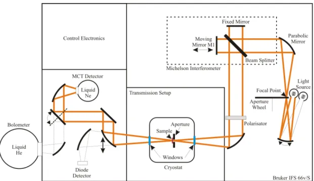
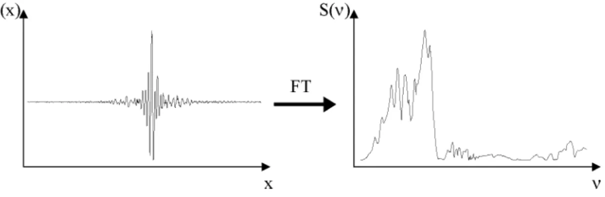
3 Fourier-Transform spectroscopy 73 3.1 Determination of the response functions . . . . 79
3.1.1 Drude-Lorentz model . . . . 79
3.1.2 Kramers-Kronig analysis . . . . 80
4 Measurements 85 4.1 Crystal-Field Excitations in VOCl . . . . 85
4.1.1 Group-Theoretical Considerations . . . . 88
4.1.2 Cluster-Model Calculations . . . 101
4.2 Phonons in hexagonal YMnO
3and YMn
0.7Ga
0.3O
3. . . 124
4.2.1 Ga Substitution . . . 126
4.2.2 Phonon Analysis . . . 127
4.2.3 Phonon Analysis of YMn
0.7Ga
0.3O
3. . . 144
4.3 Spin-lattice interactions in multiferroic MnWO
4. . . 160
4.3.1 Phonon Analysis . . . 163
4.3.2 Cluster-Model Calculations . . . 183
4.4 Phonon modes of monoclinic BiB
3O
6. . . 196
4.5 CaCrO
3, an antiferromagnetic metallic oxide . . . 207
4.5.1 Introduction . . . 207
4.5.2 Crystal Growth . . . 208
4.5.3 Crystal and Magnetic Structure . . . 208
4.5.4 LSDA and LDA+U Calculations . . . 211
4.5.5 Resistivity . . . 212
4.5.6 Optics on CaCrO
3. . . 212
5 Conclusion 233 A Wigner n-j symbols 237 A.1 3-j symbol . . . 237
A.2 6-j symbol . . . 238
A.3 9-j symbol . . . 239
Contents
B Expansion coefficients for tight-binding operator 241
List of Publications 303
Danksagung 305
Abstract 307
Zusammenfassung 309
Bibliography 311
Reference 311
Supplement 329
Offizielle Erkl¨ arung . . . 329
1 Introduction
Within the wide class of transition-metal oxides the strong correlation between elec- trons leads to unusual (often technologically useful) electronic and magnetic properties such as high-temperature superconductivity and colossal magnetoresistance. These materials are denoted as correlated electron systems, because one electron strongly influences the other ones. Since we are dealing with transition-metal oxides, these compounds have incompletely filled d or f electron shells with narrow bands and the electrons tend to localize. But in case of half-filled bands, these compounds are ex- pected to be metals, but found experimentally to be insulators. It is often not possible to use band-structure calculations to describe the electronic structure of correlated ma- terials. The application of optical spectroscopy allows the investigation of the electronic structure and the low-energetic excitations in transition-metal compounds. Further- more, optical spectroscopy can be used to probe the coupling of the electronic structure to the different degrees of freedom.
In this thesis we combined the usage of optical spectroscopy with the application of cluster-model configuration-interaction calculations. We begin with a detailed descrip- tion of a new program for doing cluster-model configuration-interaction calculations, which was developed in the framework of this thesis. In many cases configuration- interaction cluster-model calculations with full ionic multiplet structure, including crystal-field effects and covalency within a local cluster model, provide a reasonable description of the experimental results. This cluster-model configuration-interaction calculation neglects the translational symmetry and treats the local on-site electron- electron interactions explicitly. Due to the limited size of the cluster only materials with no long-range interaction can be analyzed. Metallic or half-metallic behavior cannot be described well. Typically, a cluster calculation starts with the Slater determinants of the ground configuration and the application of the creation/annihilation algebra.
But the number of Slater determinants scales drastically with increasing cluster size.
Using the Racah-Wigner algebra [1–6] and the related Wigner-Eckart theorem we can
reduce the computational effort compared with the creation/annihilation algebra. This
becomes important, if the size of the calculated cluster is more and more increased,
e.g. for double-cluster calculations. The Wigner-Eckart theorem reduces the calcula-
tion of the matrix elements of a certain operator to the calculation of a reduced matrix
element and the multiplication with a Clebsch-Gordan coefficient. The knowledge of
Slater determinants is no longer necessary and the calculation effort scales with the
number of angular momenta being involved. In order to use the Racah-Wigner algebra
we have to represent the contributions to the Hamiltonian as spherical tensor opera-
tors. Expressions for the matrix elements of the on-site Coulomb and the spin-orbit
interactions within the Racah-Wigner algebra are given by Cowan [7]. In contrast to
previous publications [8, 9] we present a general expression for the matrix elements of the crystal-field operator within the Racah-Wigner algebra, which is valid for arbitrary configurations. The application of this algebra offers an elegant and accurate descrip- tion of the electronic structure whereas the dependence of results of the cluster-model calculation on the ionic multiplets is obvious. The crystal-field operator is treated within the point-charge model, where the electrostatic field is described by the Ewald sum formulation [10]. In addition to the crystal-field operator we give an expression for the matrix elements of the covalency operator within the widely-used Slater-Koster tight-binding approximation [11] using Sobel’man’s parentage scheme [12]. The ap- plication of the Racah-Wigner algebra was not possible, because we were not able to express the tight-binding operator as a spherical tensor operator. Although So- bel’man’s parentage scheme is not as fast and elegant as the Racah-Wigner algebra, we still do not need to know the Slater determinants and conserve the dependence of the results of the cluster-model calculation on the ionic multiplet as well.
In the second part of the thesis, we begin with the analysis of the crystal-field exci- tations of the transition-metal oxyhalide VOCl by using group theoretical as well as cluster-model calculations.
The group of transition-metal oxyhalides consists of (at room-temperature) crystal- lographically iso-structural compounds and shows rather strong electron localization, resulting in (electrically) Mott-insulating properties. Within this system several elec- tronic configurations and their interactions with the crystal lattice can be probed sys- tematically.
In the following, we investigate the spin-lattice interaction in the multiferroic com- pounds h-YMnO
3and MnWO
4. We start with hexagonal YMnO
3and analyze the phonon spectra and their dependence on Ga doping by using a Drude-Lorentz model.
Replacing Mn by Ga changes the orbital occupation (from d
4to d
10) and the ionic radius. Additionally, we can achieve a better understanding of the origin of ferro- electricity in these hexagonal systems. Substituting Ga for Mn lowers also the N´ eel temperature from T
N= 72 K for YMnO
3to T
N= 35 K for YMn
0.7Ga
0.3O
3[168].
In addition, we study the temperature dependence of the phonon spectra of the mono- clinic compound MnWO
4by using a generalized Drude-Lorentz model. The spin- lattice interaction in this compound plays an important role in the coupling between antiferromagnetic and ferroelectric orders. Furthermore, we analyze the crystal-field excitations, which are strongly suppressed due to the spin-selection rule.
The understanding of the exceptional optical nonlinearities of BiB
3O
6requires a quan- titative description of the lattice dynamics. We present a detailed investigation of the linear optical response of BiB
3O
6in the phonon range for different polarizations at T
= 20 K and 300 K. We analyze the data by using a generalized Drude-Lorentz model, which allows us to obtain the frequency, the damping, the strength and the orientation of the dipole moment of each phonon mode.
We end up with a detailed investigation of the antiferromagnetic metal CaCrO
3.
Transition-metal oxides exhibit a quite general relation between magnetic order and
electrical conductivity: insulators usually exhibit antiferromagnetism, whereas ferro-
magnetism typically coexists with metallic conductivity. So observations of antifer-
romagnetic order in transition-metal oxides with metallic conductivity are of great
interest. Early electrical conductivity measurements [254, 256] show a metallic behav-
ior, whereas more recently measurements [252] indicate an insulating behavior. These
controversies are connected with the difficulty to prepare high-quality stoichiometric
materials and with the lack of large single crystals. In contrast to electrical resistivity
measurements, optical data can reveal the metallic properties of a polycrystalline metal
with insulating grain boundaries if the wavelengths are smaller than the typical grain
size.
2 Calculating the Electronic Structure of a Crystal
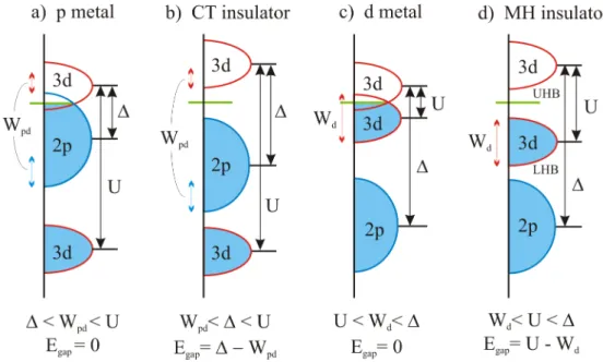
The strong electronic correlations in many transition-metal compounds with a par- tially filled 3d shell cause the insulating behavior of this materials. Within the Zaanen- Sawatzky-Allen scheme [13], these correlated systems are categorized into Mott-Hub- bard (MH) and charge-transfer (CT) insulators.
The Mott-Hubbard theory [14] involves the d − d Coulomb and exchange interactions and can be written as
H = −t X
hi,ji,σ
c
†iσc
jσ+ h.c.
+ U X
i
n
i,↑n
j,↓, (2.0.1) where n
i,↑≡ c
†iσc
iσrepresents the number operator and c
†iσcreates (annihilates) an electron on lattice site i with spin σ =↑, ↓. The first term describes the reduction of the kinetic energy of an electron by changing its position with an energy gain t. The second term represents the energy of double occupancy. The characteristic energy U is hereby defined as the repulsive Coulomb energy of two electrons on the same lattice site. The singly occupied sites will form the so-called lower Hubbard band (LHB), the doubly occupied sites form the upper Hubbard band (UHB). The size of the hopping t and the coordination number z determine the band width W . In case of a cubic system the band width is given by W = 2zt. In the limit U/t → 0, the system is metallic, because the LHB and UHB overlap and are half filled. In the other limit U/t → ∞ the system is an insulator (for half filled bands). The LHB and UHB are far away from each other and the electrons are immobile because the energy for double occupancy is very high. Within the insulating state and depending on the configuration (bond angles, orbitals,. . . ) an antiferromagnetic arrangement of neighboring spins is favored, while in the ferromagnetic case the virtual hopping is blocked by Pauli’s exclusion princi- ple.
1Since the Mott-Hubbard model can be solved analytically only in one dimension, numerical investigations in two and more dimensions contain several approximations:
The Coulomb interaction between the transition metal and its neighbored anions is neglected. Here the charge-transfer energy ∆ =
p−
d, where
ddenotes the energy of the transition-metal d orbital and
pthe energy of the ligand p orbital, has to be taken into account. This energy does not depend on U but is related to the electronegativity of the anion and the Madelung potential. Considering the charge-transfer energy, two kinds of excitations are now possible: one electron can be transferred between two transition metals, or one electron can be transferred from the ligand to a transition
1The antiferromagnetic arrangement is described by the Goodenough-Kanamori-Anderson rule [274–
276] for 180◦ superexchange.
Figure 2.1: Zaanen-Sawatzky-Allen scheme. Depending on the Coulomb repulsion U , the charge-transfer energy ∆, and the bandwidth W we get different kinds of metallic and insulating states, where W
pd=
12(W
p+ W
d). In order to be more illustrative, the hybridization in this picture is neglected. The green line indicate the Fermi energy E
F.
metal. Depending on which excitation is lower in energy, i.e. if U or ∆ is smaller, the insulator is called Mott-Hubbard insulator or charge-transfer insulator.
The Zaanen-Sawatzky-Allen scheme, shown in Fig. 2.1, depends on the Hubbard U , the charge-transfer energy ∆ and a finite band width of the d and p bands. For ∆ < U the electronic structure is dominated by the ligand band (charge-transfer type) and for
∆ > U by the 3d Hubbard band.
But even the Mott-Hubbard model, which includes the charge-transfer energy, is often inadequate in describing the full behavior of the insulating transition-metal compounds.
It is important to take the charge, lattice, orbital and spin degrees of freedom into account.
Thus, we have to consider a full multi-band theory, which includes not only the electron-
electron Coulomb repulsion. An often used calculation technique starts with a central
transition-metal cation surrounded by nearest-neighbor anions forming a cluster with
a purely ionic configuration. By using a configuration-interaction approach considering
configurations of the type d
n, d
n+1L, d
n+2LL we take hybridization and covalency as
well as the d − d Coulomb interactions into account. Here L denotes a hole in the
ligand band. The on-site energies are parameterized with U and ∆ in the same way as
done in the Zaanen-Sawatzky-Allen scheme. Within this so-called cluster-model calcu-
lation the cluster can be expressed by a matrix consisting of several configurations of
the cluster and their mixing with each other. Diagonalising the so-called “Hamilton
matrix”, we get the energies and the corresponding eigenstates of the cluster. Using the eigenstates, we can calculate the optical conductivity within the Kubo-Greenwood model and compare the results with the optical data.
In the following sections we give a detailed description of the cluster-model calcula- tion. We start with an introduction of the Hartree-Fock theory including some basic assumptions which are valid for the cluster model as well. In the following, we describe the principles of a configuration-interaction calculation and the determination of the matrix elements of one- and two-particle operators. Before we describe the determi- nation of the different parts of the Hamiltonian, we give a brief introduction to the Racah-Wigner algebra. In addition, we present some useful expressions for the calcu- lation of the matrix elements of tensor operators. The model Hamiltonian consists of four parts: The Coulomb interaction, the crystal-field splitting, the spin-orbit coupling and the covalency contribution. Furthermore, we present expressions for the matrix elements of the Stark and the Zeeman operator. We end up with the determination of the optical conductivity, the magnetic susceptibility and the phonon frequencies.
All expressions of this chapter are given in atomic units. So all energies are in rydbergs
(e
2/2a
0∼ = 13.6058 eV) and all lengths are measured in terms of the Bohr radius.
2.1 The Hartree-Fock Calculation
The calculation of the electronic structure of a crystal starts with the Hartree-Fock calculation, which is an often used approximation for solving the Schr¨ odinger equation of a many-electron system. This section contains some fundamental principles, which are valid not only for the pure Hartree-Fock calculation, but also for the cluster-model calculation, which we use for the analysis of the optical spectra. The section, which is adapted from [7], starts with a general introduction in the Hartree-Fock method and its basic assumptions. In the following we present the self-consistent field pro- cedure, which is required for solving the Hartree-Fock equations. At the end of the section, we describe the determination of the radial wave functions by solving the radial Schr¨ odinger equation numerically, which become important for the determination of several cluster-model calculation parameters such as the Slater integrals F
k, G
kand the spin-orbit coupling constant ζ.
The Schr¨ odinger equation can be solved analytically only for pure two-body systems like the hydrogen atom. For more general many-electron systems this is not possible.
But for the majority of the elements in the periodic table the motion of every electron is coupled to the motion of all other electrons as well as to the nucleus. In particular, we are interested in transition-metal compounds with strong electronic correlations within the open 3d shell. The electronic structure of such systems can be calculated only approximately.
2.1.1 Hartree-Fock Theory and Slater Determinants
The Hartree-Fock method [15] is a widely used approximation for non-correlated com- pounds. By assuming that every electron moves in the potential created both by the nucleus and by the average potential of all the other electrons, we reduces the many-electron problem to the problem of solving a number of coupled single-electron equations. The single-particle functions (orbitals, or spin orbitals) being involved in this assumption describe the motion of the electron and do not depend explicitly on the instantaneous motions of the other electrons. Only for one-electron systems the single- particle functions are exact eigenfunctions of the full electronic Hamiltonian. However, as long as we consider systems near their equilibrium, the Hartree-Fock theory provides a good description of the electronic structure of these systems.
The Hartree-Fock theory was developed in order to solve a new variant of the elec- tronic Schr¨ odinger equation which was developed from the time-independent Schr¨ o- dinger equation by making use of the Born-Oppenheimer approximation [16]. In the Born-Oppenheimer approximation the motions of the electrons are regarded as uncou- pled from those of the nuclei because of the big difference in mass. Thus the “electronic”
Schr¨ odinger equation is solved for fixed nuclear positions h T ˆ
e(r) + ˆ V
eN(r, R) + ˆ V
N N(R) + ˆ V
ee(r) i
Ψ(r, R) = EΨ(r, R). (2.1.1)
Here the symbol r denotes the electronic and the symbol R the nuclear degrees of free-
2.1 The Hartree-Fock Calculation
dom. ˆ T
erepresents the electronic kinetic energy, ˆ V
eNthe electron-nucleus interaction, V ˆ
N Nthe nuclei-nuclei interaction, and ˆ V
ee(r) the electron-electron interaction. The electronic energy eigenvalue E is a function of the chosen positions R of the nuclei.
Determine the energy for different nuclear positions we obtain the potential energy surface: E(R).
If we assume that the electrons in a N -electron system do not interact with each other ( ˆ V
ee= 0), then the Hamiltonian is separable, and the total electronic wave function Ψ(r
1, r
2, . . . , r
N) describing the motions of the electrons is the product of hydrogen wave functions χ,
Ψ
HP(x
1, x
2, · · · , x
N) = χ
1(x
1)χ
2(x
2) · · · χ
N(x
N). (2.1.2) which is known as a Hartree Product. Here, we introduced the so-called space-spin co- ordinates x = {r, σ}, with σ representing the spin coordinate. Note, that this functional form does not satisfy the antisymmetry principle, which states that a wave function describing fermions should be antisymmetric with respect to the interchange of any set of space-spin coordinates. The wave function Ψ
HPdoes not fulfill the antisymmetry principle yet. To achieve this, the wave function can be rewritten as a so-called Slater determinant [26]:
Ψ = 1
√ N !
χ
1(x
1) χ
2(x
1) · · · χ
N(x
1) χ
1(x
2) χ
2(x
2) · · · χ
N(x
2)
.. . .. . . .. .. . χ
1(x
N) χ
2(x
N) · · · χ
N(x
N)
. (2.1.3)
The use of Slater determinants guarantees the adherence to the Pauli principle: the determinant will vanish if any of the two orbitals are identical. A consequence of this functional form is that the electrons cannot be distinguished because each electron is associated with every orbital. Describing the electrons by a Slater determinant includes the assumption that each electron moves independently of all the others except that it feels the Coulomb repulsion due to the average positions of all electrons (and it also experiences an “exchange” interaction due to anti-symmetrization).
2.1.2 Self-Consistent Field Technique
The electronic Hamiltonian contains one- and two-electron operators and the nuclear repulsion term, which is constant for fixed nuclei:
H = −
n
X
i=1
1 2 ∇
2i−
N
X
k=1
Z
kr
ik! +
n
X
j=1
X
i<j
1 r
ij+
N
X
l=1
X
k<l
Z
kZ
lR
kl. (2.1.4)
Here n represents the number of electrons, N the number of nuclei and Z
ithe nuclear
charges of nucleus i. In this decomposition, the two-electron operators are critical be-
cause they prevent a product ansatz for n > 1. To circumvent this problem, Hartree has
established an approximation technique that is known as the so-called self-consistent
field (SCF) technique: The basic idea starts with the assumption that all orbitals are known and that we can determine the interaction of a single electron with all the other electrons as a mean value from their potential field. In the next step we add these mean values to the one-electron operators to obtain effective one-electron Hamiltonians
H
eff(i) = − 1 2 ∇
2i−
N
X
k=1
Z
kr
ik+ 1
2
n
X
j=1 j6=i
Z
χ
∗j1
r
ijχ
jdV
j. (2.1.5) These Hamiltonians represents the sum of all effective one-electron Hamiltonian plus the constant nuclear repulsion term:
H
el=
n
X
i=1
H
eff(i) +
n
X
l=1
X
k<l
Z
kZ
lR
kl. (2.1.6)
We can start the self-consistent field technique if we use a product of orbitals as an ansatz for the wave function. But the orbitals and the effective Hamiltonians depend on each other: We need to know the orbitals to determine the effective Hamiltonians, but we have to know the effective Hamiltonians to construct the orbitals. We can avoid this problem by using an iterative solution: We need start-orbitals ϕ(0) to form effective Hamiltonians H
eff(1), whose eigenfunctions form the orbitals ϕ(1). These imply new effective Hamiltonians H
eff(2), etc. We continue this process until the potential and the orbitals become self-consistent, which represents a good approximation for the electronic wave function Ψ
el:
Ψ
el≈
n
Y
i=1
ϕ(i). (2.1.7)
The expectation value of the electronic energy is E =
Z
Ψ
∗elH
elΨ
el= 2
n/2
X
i=1
H
i+
n/2
X
j=1
X
i<j
(2 J
ij− K
ij)
N/2
X
l=1
X
k<l
Z
kZ
lR
kl, (2.1.8) in which H
i, J
ij, and K
ijare defined as
H
i= Z
ϕ
∗i"
− 1 2 ∇
2i−
M
X
k=1
Z
kr
ik# ϕ
idV, J
ij=
Z Z
ϕ
∗i(1) ϕ
∗j(2) 1
r
ijϕ
i(1) ϕ
j(2)dV
1dV
2, K
ij=
Z Z
ϕ
∗i(1) ϕ
∗j(2) 1
r
ijϕ
j(1) ϕ
i(2)dV
1dV
2.
(2.1.9)
Note, that the self-consistent field procedure may converge to an electronically excited state, depending on the choice of the initial orbitals.
By using the variation theorem we can avoid this problem [17]: “The expectation value
of the energy is always higher than or equal to the lowest energy eigenvalue.” Due to the
2.1 The Hartree-Fock Calculation
dependence of the energy expectation value on the orbitals, we use only those values which do not change with minimal alterations of orbital values because these energy values describe the electronic ground state. This extension of the Hartree technique is known as the Hartree-Fock method.
The usage of molecular orbitals, which are defined as a linear combination of atomic orbitals:
φ
i=
m
X
j=1
C
ji· χ
j, (2.1.10)
leads to a reformulation of the Hartree-Fock method [20]. Here, the atomic orbitals χ
jdefine a m-dimensional basis of functions which are defined at the beginning and remain unchanged thereafter. The molecular orbitals’ coefficients are collected in a matrix C.
Roothaan’s ansatz limits the number of atomic orbitals and allows the application of all tools of matrix algebra due to the usage of matrices and vectors. The so-called Roothaan-Hall equations [20, 21] can be written in the form of a generalized eigenvalue problem
FC = SC, (2.1.11)
where F is the so-called Fock matrix, C is a matrix of coefficients, S is the overlap matrix of the basis functions, and is the (diagonal, by convention) matrix of orbital energies. In the case of an orthonormalized basis set, the overlap matrix S is reduced to the identity matrix.
2.1.3 Radial Schr¨ odinger Equation
Within the so-called central field approximation the effective ionic potential is spheri- cally symmetric and depends only on the magnitude of r and not on the angles θ and φ. Here the angular momentum L is classically a constant of motion. The orbital wave function χ(x) then is an eigenfunction of L
2and L
z. Thus χ(x) is a function of r times a spherical harmonics Y
lm(times a spin function). It is convenient to write the radial wave function with an explicit factor r
−1, so that the total wave function χ(x) gets the form
χ
i(x) = 1
r P
nili(r) Y
li,mli(θ, φ) σ
msi(s
z) ≡ |n
il
im
lim
sii. (2.1.12) The radial wave function P
nili(r) ≡ P
i(r) is normalized to one R
∞0
P
i∗(r)P
i(r)dr = 1 and fulfills the boundary condition P
i(r = 0) = P
i(r = ∞) = 0. The spherical harmonics Y
li,mliand the spin function σ
msi(s
z) in (2.1.12) can be exactly determined and the remaining part of the Hartree-Fock calculation is the determination of the radial wave functions P
i(r). Thus the radial Schr¨ odinger equation has to be solved
"
− d
2dr
2+ l
i(l
i+ 1) r
2− 2Z
r +
q
X
j=1
(w
j− δ
i,j) Z
∞0
2
r
>P
j2(r
2)dr
2− (w
i− 1) A
i(r)
# P
i(r)
= ε
iP
i(r) +
q
X
j=1 j6=i
w
jδ
liljij+ B
ij(r)
P
j(r),
(2.1.13)
in which
A
i(r) = 2l
i+ 1 4l
i+ 1
X
k>0
l
ik l
i0 0 0
2Z
∞ 02r
<kr
>k+1P
i2(r
2)dr
2, (2.1.14) and
B
ij(r) = 1 2
X
k
l
ik l
j0 0 0
2Z
∞ 02r
k<r
k+1>P
j(r
2)P
i(r
2)dr
2. (2.1.15) Here, Z is the charge of the nucleus, w
irepresents the number of electrons and ε
ithe binding energy of an electron in the subshell n
il
i 2. In all these integrals, the terms r
<and r
>represent the smaller and the greater value of r and r
2. The set of q equa- tions – one for each subshell n
il
i– are the Hartree-Fock equations [17–19] (HF) for the spherically averaged atom. The first two terms in (2.1.13), −d
2/dr
2+ l
i(l
i+ 1)/r
2, result from the variation of the kinetic energy and the third term refers to the nuclear potential energy. The next term refers to the direct portion of the electron-electron interactions; the terms involving A
iand B
ijrefer to the exchange portions. The terms involving the Lagrangian multipliers
ijexpress the orthogonality requirement. (In the case of closed shells, i and j , P
iand P
jare automatically orthogonal and
ijand
jican be set to zero.) Solutions of the ith HF equation are gained by trial-and-error adjustment of ε
iin order to find that value which results in a normalized solution P
i. This leads to Koopmans’ theorem [22]: “The negative form of the eigenvalue ε
iof the HF equation is equal to the configuration-averaged ionization energy of an electron in subshell n
il
i; in this case the orbitals of the ion are considered to be the same as those of the atom.”
Since the ith HF equation involves the radial wave functions P
jof all other orbitals, a set of N coupled integro-differential equations can be solved only by an iterative procedure (if N > 1). Each iterative cycle consists of three steps:
1. We assume a set of trial functions P
j(r), 1 ≤ j ≤ N .
2. For each equation i, V
H, A
iand B
ijare computed, which results in an estimate of
ij. Here V
Hrepresents the Hartree energy [23] and is defined as
V
H=
q
X
j=1
(w
j− δ
i,j) Z
∞0
2
r
>P
j2(r
2)dr
2. (2.1.16) 3. We can solve the ith HF equation to obtain a new P
i(r).
Repeating these three steps we use a new set of trial functions each time, until the out- put functions obtained in step (3) are identical with the functions assumed in step (1), and all functions with a given l are mutually orthogonal, within the desired tolerances.
The output functions are then self-consistent with the trial input functions used in
2With the sign convention,εi is negative for bound electrons and positive for free electrons.
2.1 The Hartree-Fock Calculation
computing the central field in step (2), and so this procedure is called a self-consistent- field (SCF) method. Appropriate trial input functions for the (m + 1)th iteration cycle can usually be obtained by using (normalized) linear combinations of the input and the output functions from the preceding cycle:
P
i(m+1)(input) = cP
i(m)(output) + (1 − c)P
i(m)(input). (2.1.17) The value of c is chosen by trial and error procedure in order to reach the maximum speed of convergence; usually this value is around 0.5, but it may be anywhere from 0.05 to 1.1.
The most straightforward method of finding a new output function P
i(r) in step (3) cf. (2.1.13) is the following: As a result of steps (1) and (2) everything in (2.1.13) is known with the exception of the desired function P
i(r) and the unknown parameter ε
i. We start with the boundary condition
P
i(0) = 0, (2.1.18)
which is required to keep the electron density finite at r = 0. For small values of r, all electron-electron terms in (2.1.13) are negligible compared with the kinetic and nuclear terms. The differential equation is reduced to that of a hydrogenic atom, for which P
i∝ r
li+1for small values of r. Therefore we assume an arbitrary value a
(0)0of the initial slope
a
0≡
P
i(r) r
li+1r→0
. (2.1.19)
If we begin with (2.1.18) and (2.1.19) and assume some value of ε
i, the numerical integrations
3of the differential equation (2.1.13) up to a suitably large value of r results in a particular integral P
I(r) of the inhomogeneous differential equation. If we start with the same starting conditions, the numerical integration of the homogenous differential equation, obtained from (2.1.13) by setting all
ijand B
ijto zero, results
3A commonly used method for the numerical integration of differential equations was developed by Numerov [24]: If the differential equation is written asy00=f(r)y+g(r) and ifyis already known at the pointsrj andrj−1 on a mesh in whichh=ri−ri−1 (alli), then the value ofy atrj+1 can be expressed as follows
Yj+1= 2Yj−Yj−1+h2
fjyj+ 1
12(gj+1+ 10gj+gj−1)
,
in which
Y =y
1− 1 12h2f
.
Because of numerical instabilities the integration process starts from the two boundaries of the wave function. The integration process starting at r= 0 withP(r)∝r(l+1) is called “outward”
integration. The other, starting at r = rmax with P(r) ∝ exp
−r(εi)1/2
, is called “inward”
integration. Theses two forms of integration are carried out only to a matching radius depending onεi where the outward and inward integrations produce functions with both equal values and equal slopes.
in the function P
H(r). Any integral of (2.1.13) which satisfies the above mentioned equation (2.1.18) can be written as
P
i(r) = P
I(r) + αP
H(r). (2.1.20) In this equation α is an appropriate constant, so that P
isatisfies the boundary condition
r→∞
lim [P
i(r)] = 0 (2.1.21)
required for the wave function of any bound electron; the value of the “initial slope”
of P
iis
a
0= (1 + α)a
(0)0. (2.1.22)
The value of a
0and the norm of P
i(r) depend on the assumed value of ε
i. The parameter ε
iwas originally introduced as Lagrangian multiplier associated with the normaliza- tion condition on P
i(r). It must be guaranteed that kP
i(r)k = 1. The additional requirements that a
0must be positive and that all P
i(r) have (n − l − 1) nodes lead to a unique integral P
i(r) of the HF equation (2.1.13), by analogy with the hydro- genic result. The pure Hartree-Fock method shows several disadvantages which can be avoided by using the Hartree-plus-statistical exchange approximation (HX) introduced by Cowan [25]. The HX method is an approximation to the exact HF equations and uses Hartree’s method for the self-interaction correction. The method is computation- ally much simpler and completely free of iteration-instability problems. It requires no starting parameter except an universal starting potential function. In order to approx- imate the remainder of the HF exchange terms a modification of Slater’s ρ
1/3term is used. The HX method gives results in rather good agreement with HF except for the radial wave functions P
i(r) of the inner shells, which are unimportant for all purposes except for the interaction with the nucleus.
One widely used program to do the Hartree-Fock calculation is the Cowan package
[7] based on the original Herman-Skillman program [27]. Determining the single-confi-
guration radial wave function for spherical symmetrized atoms can be done via several
homogeneous differential-equation approximations to the HF method with relativistic
corrections included.
2.2 Configuration-Interaction Method
2.2 Configuration-Interaction Method
The following section gives an introduction to the configuration interaction method, which is an essential element in the cluster-model configuration interaction calculation used in this thesis. This section is partly taken from [28].
2.2.1 Configuration Interaction
Configuration Interaction (CI) is a method for solving the time-independent Schr¨ odinger equation by using matrix mechanics. The usage of the matrix formalism simplifies the solution of the Schr¨ odinger equation Hψ = Eψ by means of a computer.
In order to apply the matrix mechanics we have to define a vector space for the descrip- tion of the problem. Within the Born- Oppenheimer approximation, we can neglect the nuclei. In case of an arbitrary N -electron system, we can express the wave function as a linear combination of all possible N -electron Slater determinants formed from a complete set of orbitals (single- particle functions). By solving the Schr¨ odinger equa- tion by using the matrix formalism on a complete basis of N -electron functions, we obtain all electronic eigenstates of the system. In case of a complete basis the electron correlation function is exactly described in contrast to the density-functional theory where only approximations are used. Within the configuration interaction method, we write a N -electron basis function |Ψi, which is a eigenvector of the Hamiltonian H, as substitutions or “excitations” of the Hartree-Fock “reference” determinant |Φ
0i, i.e.
|Ψi = c
0|Φ
0i + X
ra
c
ra|Φ
rai + X
a<b,r<s
c
rsab|Φ
rsabi + X
a<b<c,r<s<t
c
rstabc|Φ
rstabci + . . . , (2.2.1) in which |Φ
rai represents the Slater determinant formed by replacing orbital a in |Φ
0i with orbital r, etc. We can express every N -electron Slater determinant by the set of N orbitals from which it is formed. This set of orbital occupancies is often referred to as a configuration . The configuration interaction method may fail if the reference configuration is not dominant.
If we solve the Schr¨ odinger equation and use a given set of one- particle functions and all possible N -electron basis functions, the configuration interaction procedure is called
“full CI” which corresponds to solving Schr¨ odinger’s equation exactly within the space
spanned by the specified one-electron basis. If the one-electron basis is complete the
procedure is called a “complete CI” [35]. Caused by the vast number of N - electron
basis functions, a full CI can not be performed even with an incomplete one-electron
basis. Therefore, the configuration interaction space must be reduced whereas the
approximate CI wave function and its energy should be as close as possible to the
exact value. This reduction of the CI space is a central problem in the configuration
interaction theory: The most common approximation is the truncation of the CI space
expansion, “truncated CI”, according to the excitation level relative to the reference
state |Φ
0i in (2.2.1). Wave functions including only those N -electron basis functions
which represent single (Φ
ra) or double (Φ
rsab) excitations relative to the reference state
in (2.2.1). As long as the Hamilton operator includes only one- and two-electron operators, only configurations singly and doubly excited can interact directly with the reference configuration.
2.2.2 Correlation Energy
In order to estimate the quality of the configuration interaction method we can use the fraction of the correlation energy which is recovered by the truncated CI. The correlation energy is defined as
E
corr= E
0− E
HF, (2.2.2)
where E
HFrepresents the Hartree-Fock limit and E
0the exact (non-relativistic) energy of the system. The energy E
corrwill always be negative because the Hartree-Fock energy is, due to the variational theorem, an upper bound to the exact energy. The energy E
0can be calculated by performing a full CI within a complete one-electron basis set. In case of an incomplete one-electron basis set, the correlation energy represents the correlation energy of the given one-electron basis. Within the Hartree-Fock theory the inter-electron repulsion is treated only in an averaged way.
The correlation energy consits of two parts: The “dynamical” correlation energy is the energy recovered by fully allowing the electrons to avoid each other. The second part, called the “non- dynamical”, or “static” correlation energy, re?ects the inadequacy of a single reference in describing a given (molecular) state, and is due to nearly degenerate states or rearrangement of electrons within partially ?lled shells.
2.2.3 Truncated Configuration Interaction
The CI expansion is typically truncated according to its excitation level. The structure of the CI matrix with respect to its excitation level is given below [34]. |Si, |Di, |T i and |Qi represent blocks of singly, doubly, triply, and quadruply excited determinants, respectively. The Hamiltonian H is Hermitian; in case of exclusively real orbitals, the Hamiltonian is also symmetric. Thus only the lower triangle of H is shown below
H = hΦ
0|
hS|
hD|
hT | hQ|
.. .
hΦ
0|H|Φ
0i . . .
0 hS|H|Si . . .
hD|H|Φ
0i hD|H|Si hD|H|Di . . . 0 hT |H|Si hT |H|Di hT |H|T i . . . 0 0 hQ|H|Di hQ|H|T i hQ|H|Qi . . .
.. . .. . .. . .. . .. . . ..
. (2.2.3)
Due to Brillouin’s theorem [39] the matrix elements hS|H|Φ
0i are zero, which is valid when the reference function |Φ
0i is obtained by the Hartree-Fock method
4. Further- more, the blocks hX|H|Y i which are not necessarily zero may still be sparse; for ex- ample, the matrix element hΦ
rsab|H|Φ
tuvwcdefi which belongs to the block hD|H|Qi, will
4“Hartree-Fock guarantees that off-diagonal elements of the Fock matrix are zero. It turns out that the matrix element between two Slater determinants which differ by one spin orbital is equal to an off-diagonal element of the Fock matrix.”, see [30].
2.2 Configuration-Interaction Method
be non-zero only if a and b are contained in the set {c, d, e, f } and if r and s are contained in the set {t, u, v, w}. Double excitations make the largest contributions to the CI wave function besides the reference state, since they interact directly with the Hartree-Fock reference. Although singles, triples, etc. do not interact directly with the reference state, they can still become part of the CI wave function (i.e. they have non-zero coefficients) because they mix with the doubles, directly or indirectly.
The number of N -electron basis functions increases dramatically if the excitation level is increased. So the CISDTQ method is limited to systems containing very few heavy atoms. Full CI calculations are of course even more difficult to perform, so that in spite of their importance as benchmarks, only few full CI energies using flexible one-electron basis sets have been obtained. If spatial symmetry is ignored the dimension of the full CI space with total spin S is computed by
D
n N S=
n N/2 + S
n N/2 − S
, (2.2.4)
in which n denotes the number of orbitals and N the number of electrons.
In the often used frozen-core approximation the lowest-lying ionic orbitals (occupied by the inner-shell electrons) are constrained to remain doubly-occupied in all configu- rations. For the atoms ranging from Lithium to Neon the frozen core typically consists of the 1s atomic orbital, while the frozen-core for those atoms ranging from Sodium to Argon consists of the atomic orbitals 1s, 2s, 2p
x, 2p
yand 2p
z. The inner-shell electrons of an atom are less sensitive to their environment than the valence electrons.
Thus the error introduced by freezing the core orbitals is generally small. Applying the frozen core approximation, we can decrease the number of configurations within the configuration interaction method and reduce the computational effort to construct the Hamiltonian. Truncating the CI space will introduce an error in the wave functions, in the related energies and all other properties. Furthermore the CI energies are no longer size extensive
5or size consistent
6. The truncated configuration interaction method is neither size extensive nor size consistent. Due to the lack of the property of size ex- tensivity, the accuracy of a truncated configuration interaction calculation decrease with increasing system size. In order to correct the CI energies Davidson suggests the following correction [41]
∆E
DC= E
SD(1 − c
0), (2.2.5)
where E
SDis the basis set correlation energy recovered by a CISD procedure and c
0is the coefficient of the Hartree-Fock wave function in (2.2.1). This correction approxi- mately accounts for the effects of “unlinked quadruple” excitations (i.e. simultaneous pairs of double excitations).
5A calculation method is size extensive if the energy calculated thereby scales linearly with the number of particlesN.
6A method is called size consistent if there exists an energy ε = EA+EB which consists of two well separated subsystemsAandB. In contrast to the definition of size extensivity, which applies at any geometry, the definition of size consistency applies only in the case of infinite separation.
Furthermore, size consistency usually implies correct dissociation into fragments, too.
2.3 Coupled Antisymmetrized Basis Functions
This section, which follows the explanations of Cowan [7], introduces several expressions which are valid for the cluster-model calculation. We begin with the construction of the wave functions used in the configuration interaction calculation and end up with the principle determination of matrix elements of one- and two-electron operators. This is important, because the usage of one- and two-electron operators avoids the complete antisymmetrization of the wave functions. Without these fundamental considerations we cannot calculate the Hamiltonian within the configuration interaction method. In addition, the so-called “coefficients of fractional parentage”, which are defined in this section, are an essential component of Sobel’man’s parentage scheme approximation used in the determination of the tight-binding operator (see section “2.8 Hybridization and Tight-Binding Approximation”).
2.3.1 Coefficients of Fractional Parentage
Basis wave functions for a N -electron atom are constructed from linear combinations of products of N one-electron orbitals (2.1.12). If we do not couple the angular momenta together, we can achieve antisymmetrized wave functions by forming determinantal functions:
ψ = 1
√ N ! X
P
(−1)
pN
Y
i=1
|n
il
im
lim
si(r
j)i, (2.3.1) in which the summation runs over all N ! permutations of the coordinate subscripts j, and p is the parity of the permutation P . To guarantee a properly normalized function the factor (N !)
−1/2is required.
To construct multiplet wave functions of a subshell nl
w|l
w, α, L, S, M
L, M
Si, (2.3.2) with w denoting the number of electrons in the subshell nl, we have to couple the angular momenta of the different orbitals according to some coupling scheme. Here α distinguishes between multiplets with the same L and S quantum numbers, which could be found for example within a 3d
3subshell, in which two multiplets with L = 2 and S =
12exist. The quantum numbers M
Land M
Sin (2.3.2) represents the mag- netic quantum numbers corresponding to L and S respectively. The coupling of the angular momenta is done with the aid of the Clebsch-Gordan (CG) coefficients. The application of Clebsch-Gordan expansions to antisymmetrized product functions may lead to normalization difficulties if two or more electrons are equivalent (n
il
i= n
kl
k).
We can avoid these difficulties by using appropriate linear combinations of coupled
simple-product functions which are not antisymmetrized. These combinations are in-
dependent of M
Land M
S, which are therefore dropped from notation. If |l
w−1α L Si
is an antisymmetric basis function for a subshell nl
w−1with w − 1 equivalent electrons
2.3 Coupled Antisymmetrized Basis Functions
and α L S indicating a multiplet within this subshell, and if
7| l
w−1α L S, l
LSi = X
MLml
CG LlM
Lm
l; LM
LX
SLms
CG SsM
Sm
s; SM
S× |l
w−1α L Si |li
(2.3.3) is a coupled but not antisymmetrized function, then a completely antisymmetric func- tion |l
wαLSi for subshell nl
wcan be written in terms of the coefficients of fractional parentage
8(cfp) denoted by “ l
w−1α L S|}l
wαLS
”, which were introduced by Racah [5]
|l
wαLSi = X
α L S
| l
w−1α L S, l
LSi l
w−1α L S|}l
wαLS
. (2.3.4)
The coefficients of fractional parentage describe how the antisymmetric multiplet wave function |l
wαLSi of subshell nl
wis constructed by the multiplet wave functions of sub- shell nl
w−1by adding a further electron via angular momentum coupling.
Antisymmetric functions for an arbitrary subshell with w electrons are in principle constructed by repeated application of (2.3.4), starting with w = 2. The terms α L S are called parent terms for the terms αLS.
The coefficients of fractional parentage satisfy the relations [7]
X
α L S
l
wα L S{|l
w−1α L S
l
w−1α L S|}l
wα
0L S
= δ
α,α0, (2.3.5) due to orthonormalization, and
X
αLS
[L, S] l
w−1α L S|}l
wα L S
l
wα L S{|l
w−1α
0L S
= 1
w (4l + 3 − w) L, S
δ
α,α0, (2.3.6) which is useful for checking the correctness of the calculated values of the cfp. A complete set of tables is given by Nielson and Koster [45].
2.3.2 Basis Functions within the Russell-Saunders-coupling scheme
The above presented procedure gives completely antisymmetrized wave functions for a subshell with w equivalent electrons. But within the configuration-interaction calcu- lation, we have to deal with configurations which contain different subshells. For an
7The expression| lw−1α L S, l
LSi represents a multiplet wave function of subshellnlw with mul- tipletLS, which is constructed from the mutliplet wave function of subshellnlw−1, with multiplet indicated byα L S, by adding a further electron with angular momentumlto this wave function.
The sums run on the one hand over the corresponding magnetic quantum numberML andMS
of the mutlipletα L Sand on the other hand over the magnetic quantum numbersml andmsof the added electron. The CG expressions represent the Clebsch-Gordan coefficients, which describe the adding ofl toLandsto S respectively. Finally, the expression|liis the single-electron wave function of the added electron.
8Racah’s notation
lw−1α L S, l
αLS|}lwαLS
is redundant.
![Figure 4.4: Tanabe-Sugano diagram for a d 2 configuration in a cubic environment [148]](https://thumb-eu.123doks.com/thumbv2/1library_info/3699840.1505960/103.892.223.650.132.447/figure-tanabe-sugano-diagram-for-configuration-cubic-environment.webp)
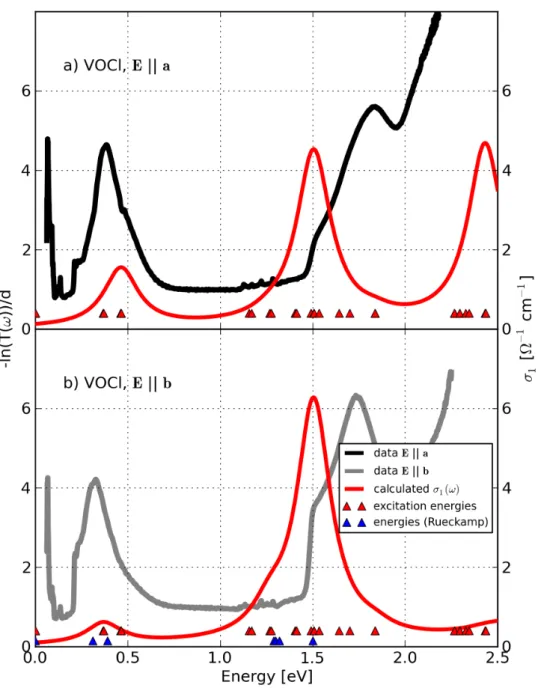
![Figure 4.20: Comparison between the measured absorption −ln(T (ω))/d (grey and light grey lines) determined by R¨ uckamp [135] and the calculated opti-cal conductivity σ 1 (ω) (solid lines) of TiOCl for T = 295 K for Eka (grey color) and Ekb (light grey c](https://thumb-eu.123doks.com/thumbv2/1library_info/3699840.1505960/131.892.179.693.168.833/figure-comparison-measured-absorption-determined-uckamp-calculated-conductivity.webp)
![Table 4.10: Atomic site symmetries and irreducible representations for the atoms in hexagonal YMnO 3 [152].](https://thumb-eu.123doks.com/thumbv2/1library_info/3699840.1505960/137.892.136.740.127.324/table-atomic-symmetries-irreducible-representations-atoms-hexagonal-ymno.webp)
