Optimizing Time-series Forecasts for Inflation and Interest Rates Using Simulation and Model Averaging

IHS Economics Series Working Paper 231

November 2008

Optimizing Time-series Forecasts for Inflation and Interest Rates Using Simulation and Model Averaging

Adusei Jumah

Robert M. Kunst

Impressum Author(s):

Adusei Jumah, Robert M. Kunst Title:

Optimizing Time-series Forecasts for Inflation and Interest Rates Using Simulation and Model Averaging

ISSN: Unspecified

2008 Institut für Höhere Studien - Institute for Advanced Studies (IHS) Josefstädter Straße 39, A-1080 Wien

E-Mail: o ce@ihs.ac.atffi Web: ww w .ihs.ac. a t

All IHS Working Papers are available online: http://irihs. ihs. ac.at/view/ihs_series/

This paper is available for download without charge at:

https://irihs.ihs.ac.at/id/eprint/1877/

Optimizing Time-series Forecasts for Inflation and Interest Rates Using Simulation and Model Averaging

Adusei Jumah, Robert M. Kunst

231

Reihe Ökonomie

Economics Series

231 Reihe Ökonomie Economics Series

Optimizing Time-series Forecasts for Inflation and Interest Rates Using Simulation and Model Averaging

Adusei Jumah, Robert M. Kunst November 2008

Institut für Höhere Studien (IHS), Wien

Institute for Advanced Studies, Vienna

Contact:

Adusei Jumah

Department of Economics and Finance Institute for Advanced Studies Stumpergasse 56

1060 Vienna, Austria and

Department of Economics University of Vienna Brünner Strasse 72

1210 Vienna, Austria

email: adusei.jumah@univie.ac.at

Robert M. Kunst

Department of Economics and Finance Institute for Advanced Studies Stumpergasse 56

1060 Vienna, Austria and

University of Vienna Department of Economics Brünner Straße 72 1210 Vienna, Austria

email: robert.kunst@univie.ac.at

Founded in 1963 by two prominent Austrians living in exile – the sociologist Paul F. Lazarsfeld and the economist Oskar Morgenstern – with the financial support from the Ford Foundation, the Austrian Federal Ministry of Education and the City of Vienna, the Institute for Advanced Studies (IHS) is the first institution for postgraduate education and research in economics and the social sciences in Austria.

The Economics Series presents research done at the Department of Economics and Finance and aims to share “work in progress” in a timely way before formal publication. As usual, authors bear full responsibility for the content of their contributions.

Das Institut für Höhere Studien (IHS) wurde im Jahr 1963 von zwei prominenten Exilösterreichern – dem Soziologen Paul F. Lazarsfeld und dem Ökonomen Oskar Morgenstern – mit Hilfe der Ford- Stiftung, des Österreichischen Bundesministeriums für Unterricht und der Stadt Wien gegründet und ist somit die erste nachuniversitäre Lehr- und Forschungsstätte für die Sozial- und Wirtschafts- wissenschaften in Österreich. Die Reihe Ökonomie bietet Einblick in die Forschungsarbeit der Abteilung für Ökonomie und Finanzwirtschaft und verfolgt das Ziel, abteilungsinterne Diskussionsbeiträge einer breiteren fachinternen Öffentlichkeit zugänglich zu machen. Die inhaltliche Verantwortung für die veröffentlichten Beiträge liegt bei den Autoren und Autorinnen.

Abstract

Motivated by economic-theory concepts—the Fisher hypothesis and the theory of the term structure—we consider a small set of simple bivariate closed-loop time-series models for the prediction of price inflation and of long- and short-term interest rates. The set includes vector autoregressions (VAR) in levels and in differences, a cointegrated VAR, and a non-linear VAR with threshold cointegration based on data from Germany, Japan, UK, and the U.S.

Following a traditional comparative evaluation of predictive accuracy, we subject all structures to a mutual validation using parametric bootstrapping. Ultimately, we utilize the recently developed technique of Mallows model averaging to explore the potential of improving upon the predictions through combinations. While the simulations confirm the traded wisdom that VARs in differences optimize one-step prediction and that error correction helps at larger horizons, the model-averaging experiments point at problems in allotting an adequate penalty for the complexity of candidate models.

Keywords

Threshold cointegration, parametric bootstrap, model averaging

JEL Classification

C32, C52, E43, E47

Contents

1 Introduction 1

2 Statistical evidence 3

2.1 The data... 3

2.2 Testing for unit roots ... 6

2.3 Cointegration tests... 7

3 Simple forecasting experiments 8

3.2 Short rate and inflation... 13

3.3 Long rate and inflation ... 14

3.4 Performance across all models ... 14

4 Bootstrap validation 15

5 Model averaging 18

6 Summary and conclusion 22

References 24

1 Introduction

We consider a hypothetical forecaster whose information set is restricted to time series of two interest rates at different maturities and a rate of price inflation at a quarterly frequency. Her task is to generate predictions of the three variables that are as close to the realized values as possible. Her tool- box consists of four bivariate time-series models, three linear models and a nonlinear structure. Primarily we focus on the task of selecting the best pure model but we also consider the possibility of combining several candidates.

The forecaster’s choice of the four candidates is inspired by economic theory, namely the Fisher hypothesis and the theory of the term structure.

In their econometric interpretation, these concepts translate into stationary differences between any two of the variables, while the variables themselves are often considered as first-order integrated (I(1))—a cointegrated system (see Engle and Granger , 1987). This paper investigates the extent to which these theoretical concepts are able to assist the forecaster.

Particularly the idea of cointegration among interest rates at different maturities has been supported by the seminal contribution of Campbell and Shiller (1987). It also appears as a building block of many current macroeconomic models. For a critique of this approach, see for example Malliaropulos (2000) who views inflation as well as interest rates as trend- stationary but subject to rare trend breaks. For a forecaster, however, such concepts are unattractive as they require a prediction of the timing of the breaks. We confine ourselves to time-homogeneous models exclusively.

We contrast the error-correction model (EC-VAR in short) with three other time-series models of comparable complexity. A simple VAR in lev- els expresses the possibility that all variables are stationary in a longer-run perspective. This view is not implausible, given the observation that both interest rates and rates of inflation remain in a bounded region over time spans of several decades. Second and conversely, a VAR in differences un- derscores the short-run nature of the variables that may be reminiscent of random walks or at least of first-order integrated series, while it deliberately ignores the equilibrium restrictions imposed by the Fisher effect and the mean-reverting term structure. As a stark contrast and some kind of freak- ish alien, we construct a threshold VAR as the fourth candidate. It behaves like the EC-VAR in the distributional center of the variables but changes to the stable VAR in its outer region, for unusually high or low rates of interest and of inflation. At the outset, we conjectured that this model, globally sta- ble according to statistical theory but locally unstable, might capture most features of time-series behavior that we observe in the data. Threshold mod- els of similar type were suggested by Balke and Fomby (1997), although

1

with a slightly different view of the corridor problem. Their model cointe- grates but ignores small deviations from long-run equilibrium paths. Our model cointegrates in the corridor, i.e. in the center, but develops a globally stable regime in its tails.

We emphasize that we do not intend to prove or disprove economic theo- ries. The mentioned concepts—the Fisher effect and the term structure—are far more flexible than our simple time-series models and allow for longer-run variation in term premia as well as in ‘natural’ real rates. They also may be designed to hold contingent on exogenous environment designs and political circumstances, which is a view that we rule out in ‘closed-loop’ modelling, as we think it gets too arbitrary in a prediction evaluation. However, the models we use are simplified and not uncommon operational counterparts of these theoretical ideas. In short, the theory may hold for whatever model of our foursome that comes out best in the prediction evaluation. Moreover, we do not even intend to find true or valid models. As we set out above, incorrect models can be excellent forecasting ‘workhorses’, while correct parametric models fitted to samples of finite length may yield disappointing forecasting performance. The mismatch of statistical in-sample evidence and of fore- casting performance has repeatedly inspired the literature. Recently, it was picked up in noteworthy contributions by Granger (2005) and by Arm- strong (2007).

Our test data are samples over several decades on Germany, Japan, UK, and the U.S. These are four major economies of widespread relevance, and results on them may be viewed as role-model cases. The samples cover the episode of high inflation and interest following the OPEC shocks of the 1970s and are therefore representative of the typical behavior over longer time spans that will always show calm ‘textbook’ phases and ‘wild’ episodes that do not correspond to textbook wisdom.

There is no universally accepted technique for model selection with the aim of forecasting. Statistical in-sample techniques may be inadequate, as neither the arbitrary 5% significance level of hypothesis tests nor the back- drop aim of searching for correctness in the specification may be well adapted to the prediction purpose. For this reason, statistical in-sample evidence is presented only briefly. Rather, we tend to rely on comparisons over test samples, which are presented in Section 3.

Additional information may be obtained using a more advanced concept of parametric bootstrap validation that is enacted in Section 4. The tech- nique appears rudimentarily in some of the forecasting literature but it was introduced as a tool explicitly by Jumah and Kunst (2008) and Kunst (2008). Under the assumption of any of the four candidates as the data- generating process (DGP), pseudo-samples are simulated, and again each

2

model class is applied as a prediction model generator. The results yield information about the robustness of forecasting performance with regard to uncertain model assumptions.

Finally, we consider the recently developed model-averaging technique by Hansen (2007). Here, relative weights on each of the candidate model classes are taken as indicators of the relative importance of the class with regard to prediction. This strategy is motivated by the fact that the original Hansen procedure is inspired by prediction concepts. However, it turns out that the resulting combined forecast construct rarely beats the pure model-based predictions evaluated before.

The remainder of this paper is organized as follows. Section 2 describes the data and briefly reviews some statistical in-sample evidence, although we do not rely too much on it in a forecasting project. Section 3 reports the basic prediction horse race among the four rival models. Section 4 deals with the slightly more sophisticated technique of parametric bootstrap vali- dation. Section 5 considers combinations across the four basic rival models and reports fitted in-sample weights. Section 6 concludes.

2 Statistical evidence

2.1 The data

For our analysis, we need time series on inflation and on interest rates for different terms to maturity. With regard to inflation, the choice of the appro- priate indicator is simple, as most economies have reliable series for longer time spans on consumer prices only. Given such a consumer price index P

, inflation is appropriately defined as π

= Δ

p

, where the lower-case p de- notes the logarithm of the original variable P . Throughout, we use Δ for the first differences operator and Δ

for annual quarter-to-quarter differences, i.e. Δ X

= X

− X

and Δ

X

= X

− X

for any given variable X . The selection of appropriate variables is much harder for interest rates. Mainly for reasons of comparability across countries and data availability, we selected a short-term money-market rate i

and a longer-term bond rate i

.

In order to enhance the significance of our findings, we study all effects in parallel for four main economies: Germany (the Federal Republic before German unification), the United States, the United Kingdom, and Japan.

Figures 1 to 4 convey an impression of the data at hand. All data are taken from the IFS data base compiled by the International Monetary Fund. For time ranges, we use the longest available ones, i.e. samples end in 2007:4 and start in 1960:4 for Germany and the United States, in 1972:1 for the United

3

Figure 1: Long ( i

, solid) and short ( i

, dashed) interest and price inflation ( π , short dashes) for Germany.

Kingdom, in 1966:4 for Japan.

Whereas economic theory defines the real interest rate as the forward- looking interest i

minus the expected inflation instead of the backward- looking inflation π

, this definition of the real rate is inconvenient for data- driven prediction. Also the customary alternative ex-post real interest rate i

− π

is inconvenient for prediction analysis. We note that the distinction between the ‘correct’ ex-post real rate and the ‘incorrect’ or naive real rate i

− π

is unimportant with regard to cointegration properties. Contingent on I(1) properties for inflation and interest, the ex-post real rate is I(0) and the variables therefore cointegrate if and only if the same holds for the naive rate.

According to this convention, we view the difference between an interest rate and inflation as the ‘real rate’, while the difference i

− i

is the ‘term premium’. Figures 1 to 4 show important similarities across countries. For most of the time, i

lies above i

, which in turn typically exceeds inflation, such that both the real rate and the term premium tend to be positive. The figures also show that generally a high-volatility time period with remarkable peaks around 1980 is followed by a calmer period with lower values up to the present.

Apart from this visual evaluation, some more detailed statistical char- acteristics will be reported in the next subsections. As motivated in the introduction, we report on all of these in-sample statistics only summarily, as they may not be too relevant for the aim of prediction.

4

Figure 2: Long ( i

, solid) and short ( i

, dashed) interest and price inflation ( π , short dashes) for the United States.

Figure 3: Long ( i

, solid) and short ( i

, dashed) interest and price inflation ( π , short dashes) for the United Kingdom.

5

Figure 4: Long ( i

, solid) and short ( i

, dashed) interest and price inflation ( π , short dashes) for Japan.

2.2 Testing for unit roots

Table 1: Statistical evidence for unit roots.

Germany United States United Kingdom Japan

i

0(2) 0(3) 1(0) 1(1)

i

1(1) 1(1) 1(1) 1(1)

π 1(4) 0(8) 1(8) 1(8)

Note: Numbers indicate identified integration order according to Dickey- Fuller tests at the 5% significance level. Numbers in brackets indicate aug- mentation lag order selected by Schwarz criterion.

Table 1 summarizes the results from customary statistical unit-root tests according to Dickey and Fuller (1979). These tests reject a unit root for the UK short-term rate at the 10% level and at 5% for the German and U.S.

short rates, but support it for the long rates as well as for the Japanese series.

Control procedures using refined unit-root tests draw a similar picture.

Inflation data are predominantly found to be ‘statistically I(1)’ in the sense that Dickey-Fuller tests do not reject their null. For Germany, however, the statistic comes close to the 10% significance point, and for the U.S., it even rejects the unit root at 1%.

In summary, both interest rates and inflation are located at both sides of

6

the statistical boundary of unit-root tests, confirming the visual impression as well as our theoretical concerns. Moreover, all results are sensitive to changes in the sample range.

Results on the differences i

−i

, the term premium, and i

−π and i

−π , the real rates, are also inconclusive. Tests for these series tend to reject the unit-root null more often than for the original variables but generally the values of the statistics again cluster around the significance points.

2.3 Cointegration tests

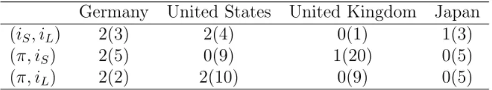
Table 2: Statistical evidence for cointegration.

Germany United States United Kingdom Japan

( i

, i

) 2(3) 2(4) 0(1) 1(3)

( π, i

) 2(5) 0(9) 1(20) 0(5)

( π, i

) 2(2) 2(10) 0(9) 0(5)

Note: Numbers indicate the cointegrating rank identified by Johansen tests at 5% significance level. Numbers in brackets indicate VAR lag order selected by AIC.

Table 2 summarizes the results of statistical VAR cointegration tests ac- cording to Johansen (1995). We confine ourselves to commenting on some of the cases.

For Germany, a system consisting of the two interest rates has VAR order 3 according to an AIC lag-order search. There is convincing support for at least one cointegration vector and 5% support for another one, which would yield a fully stationary system, contradicting univariate evidence. The parallel U.S. system behaves similarly to the German one. One cointegration vector is significant at extreme levels, and the other one at an approximate 3%

level. By contrast, the bivariate system for Japan supports one vector clearly, and the one for the United Kingdom does not support any cointegration at all.

The general impression is a confusing variety across countries: pure I(1) in the United Kingdom, theory-supported cointegration in Japan, and ‘al- most’ stationary systems in Germany and the U.S. Taken literally, these results would support modelling in differences for Germany, error-correction modelling for Japan, and ‘level’ VARs for the other two cases.

For the short rate and inflation in Japan, no cointegration is supported and a pure I(1) structure is identified, even though formally the error-correction

7

model is rejected against the alternative of a stationary model. In the paral- lel U.K. system with its extraordinary lag length, one cointegration vector is supported at extreme significance, another one at around 7%. For the U.S.

( π, i

) system, one cointegration vector is marginally significant at around 6%, another one is formally ‘supported’ at 2%.

In summary, test statistics tend to be close to the significance boundaries in the ( π, i

) systems, such that the hypotheses of no, one, and even two cointegrating vectors are not separated clearly. The impression is comparable for the ( π, i

) systems. Pure I(1) non-cointegrated structures are supported for Japan and also for the ( π, i

) system in the UK.

Generally, the statistical classification of variables varies considerably across countries and it is sensitive to changes in the sample range. The model with the best support in the literature, the error-correction model with one cointegrating vector, is found only in two out of 16 cases. Note, however, that even the protagonists of the cointegrating model for the term structure, Campbell and Shiller (1987), reported empirical deviations from the error-correction concept. Our Table 2 should not be interpreted as evidence for discarding that concept.

3 Simple forecasting experiments

For all four countries, we construct predictions as follows. Vector autore- gressions and VAR models in first differences are fitted to the observations at time points t for t ≤ n − m if n is the last available observation of the series. Then, the data point at t = n − m + 1 is predicted by its conditional expectation, given the specified model in usage. This exercise is repeated for m = 1 , . . . , 40, such that single-step out-of-sample predictions are calculated for the last ten years in the sample. Generally, for all considered time-series models lag orders are determined by an AIC search up to p = 12, individually for each time range.

Let ( y

) denote the bivariate process that consists alternatively of two interest rates or of an interest rate and the rate of inflation. Prediction models under consideration are:

1. the VAR in ‘levels’ y

= μ +

j=1

Φ

y

+ ε

. If fitted to data, this model tends to yield ‘stable’ coefficient estimates such that det(I −

j=1

Φ

z

) has zeros for |z| > 1 only. Then, there are no ‘unit roots’

and ( y

) is an asymptotically stationary process.

2. the VAR in differences (dVAR) Δ y

= μ +

j=1

Φ

Δ y

+ ε

. This model imposes 2 unit roots in bivariate systems and excludes the pos-

8

sibility of cointegration. If det(I −

j=1

Φ

z

) has zeros for |z| > 1 only, ( y

) is a first-order integrated process with two unit roots in the lag polynomial.

3. the error-correction VAR (EC–VAR) Δ y

= μ + αβ

y

+

j=1

Φ

Δ y

+ ε

, with the restriction β = (1 , − 1)

. Under some additional regular- ity conditions, this model has one unit root and yields a first-order integrated ( y

).

4. the threshold cointegration model (th-VAR)

Δ y

= μ + α

β

y

+ α

β

y

I ( |β

y

− η| > c ) +

j=1

Φ

Δ y

+ ε

with the restrictions β

= (1 , − 1)

, β

= (0 , 1)

or (1 , 0)

.

The threshold model is the most sophisticated structure and deserves some comments. Note that it is of crucial importance that the second error- correction variable β

y and the transition variable coincide. This ensures that the variable y

is stochastically bounded on a compact set and geometrically stable on its complement. These assumptions suffice to prove the geomet- ric ergodicity and stability of the variable ( y

), a feature that was observed by Tong (1990). The model is different from most threshold cointegra- tion models that can be found in the econometric literature (see, e.g., de Gooijer and Vidiella-i-Anguera , 2004), due to its switching integra- tion order across regimes. It is comparable to the class studied by Rahbek and Shephard (2002) and it produces, in line with these authors, ‘epochs of seeming non-stationarity ... before they collapse back toward their long-term relationship’. This implies that most econometric methods suggested in the literature are not well suited for this model class. In particular, multi-stage model building procedures that start by testing for linear cointegration may not be adequate.

At this stage, it does not make sense to be more specific on the properties of the error process ( ε

). A maximal assumption is that it is Gaussian white noise, which will be adopted for the simulation experiments. A minimum as- sumption would be a martingale-difference sequence with constant and finite variance. For a recent general treatment of stability conditions of nonlinear dynamic models, which comprises the th-VAR model as a special case, see Liebscher (2005).

The candidate models VAR, dVAR, EC-VAR, and th-VAR constitute a partially nested set. The dVAR restricts the EC-VAR by excluding the error- correction term, while the EC-VAR restricts the VAR by imposing a rank

9

restriction on the ‘impact matrix’. Formally, the th-VAR model encompasses the EC-VAR structure but our specific search for the thresholds does not admit the restricted linear model. Similarly, the lag order is determined for each of the individual models separately, such that the utilized model sets conditional on lag orders are typically not nested. Thus, for example the dVAR specification used as a prediction model may have a higher parameter dimension than the VAR candidate.

Prediction using the models VAR, dVAR, and EC-VAR is straight for- ward. The parameters are estimated by least squares, and the mean predic- tion is obtained by evaluating conditional expectation. Again, the th-VAR model deserves some comments. Given c and η , all parameters can be ef- ficiently estimated by least squares. To estimate c and η , we use a crude grid and optimize in-sample performance over the quantiles of β

y

for β

= (0 , 1)

and (1 , 0)

at position 0 . 05 j, j = 1 , . . . , 5 and at the upper posi- tions 1 − 0 . 05 j, j = 1 , . . . , 5.

The th-VAR model is nonlinear, and substituting parameter estimates to its right-hand side does not yield the approximate conditional expectation.

For this reason, we draw 100 trajectories based on Gaussian errors with estimated σ and average them to obtain our mean forecast.

We base the evaluation of predictive accuracy on univariate measures, such as the mean squared error (MSE) for single variables, exclusively. All MSE evaluations were accompanied by unreported evaluations using different loss criteria, such as the mean absolute error (MAE). The ranking of models proved to be robust with regard to changes in the loss criterion. Bivariate criteria were not considered, in line with the assumed forecaster’s objective.

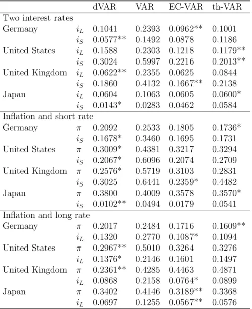
3.1 Two interest rates

Generally, lag orders coincide with those reported in Table 2. Table 3 shows that the performance of the dVAR is markedly better than that of the levels VAR. Note that this outcome is in line with the statistical evidence for the United Kingdom only.

If the data is handled as cointegrated with the pre-determined cointe- grating vector i

− i

, forecasting performance is competitive with the dVAR and VAR models for the long rate i

but much less so for i

. Note that statistical methods find at least one cointegrating vector for all cases except for the U.K. However, the EC-VAR forecast performs pretty well just for the U.K., where it dominates the i

prediction and is beaten at hair’s width for the i

prediction.

The last model whose forecasting performance we explore is the thresh- old cointegration model with a stabilizing second cointegrating vector that is

10

Table 3: Mean squared errors (MSE) for single-step prediction.

dVAR VAR EC-VAR th-VAR

Two interest rates

Germany i

0.1041 0.2393 0.0962** 0.1001 i

0.0577** 0.1492 0.0878 0.1186 United States i

0.1588 0.2303 0.1218 0.1179**

i

0.3024 0.5997 0.2216 0.2013**

United Kingdom i

0.0622** 0.2355 0.0625 0.0844 i

0.1860 0.4132 0.1667** 0.2138

Japan i

0.0604 0.1063 0.0605 0.0600*

i

0.0143* 0.0283 0.0462 0.0584 Inflation and short rate

Germany π 0.2092 0.2533 0.1805 0.1736*

i

0.1678* 0.3460 0.1695 0.1731 United States π 0.3009* 0.4381 0.3217 0.3294 i

0.2067* 0.6096 0.2074 0.2709 United Kingdom π 0.2576* 0.5719 0.3103 0.2831 i

0.3025 0.6441 0.2359* 0.4482

Japan π 0.3800 0.4009 0.3578 0.3570*

i

0.0102** 0.0494 0.0179 0.0541 Inflation and long rate

Germany π 0.2017 0.2484 0.1716 0.1609**

i

0.1320 0.2770 0.1087* 0.1094 United States π 0.2967** 0.5010 0.3264 0.3276 i

0.1376* 0.2146 0.1601 0.1497 United Kingdom π 0.2361** 0.4285 0.4463 0.4871 i

0.0868 0.2158 0.0764* 0.0899

Japan π 0.3402 0.4146 0.3189** 0.3368

i

0.0697 0.1255 0.0567** 0.0576

Note: one asterisk denotes the best specification among the specific bivariate models, two asterisks denote the best specification for the variable.

11

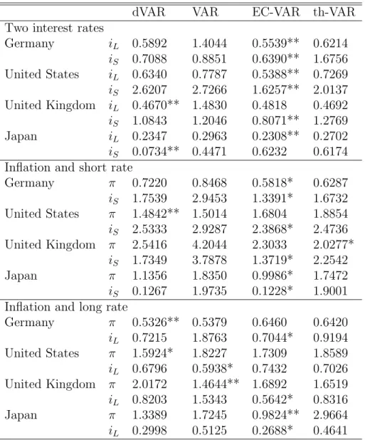
Table 4: Mean squared errors (MSE) for four-step prediction.

dVAR VAR EC-VAR th-VAR

Two interest rates

Germany i

0.5892 1.4044 0.5539** 0.6214 i

0.7088 0.8851 0.6390** 1.6756 United States i

0.6340 0.7787 0.5388** 0.7269 i

2.6207 2.7266 1.6257** 2.0137 United Kingdom i

0.4670** 1.4830 0.4818 0.4692 i

1.0843 1.2046 0.8071** 1.2769

Japan i

0.2347 0.2963 0.2308** 0.2702

i

0.0734** 0.4471 0.6232 0.6174 Inflation and short rate

Germany π 0.7220 0.8468 0.5818* 0.6287

i

1.7539 2.9453 1.3391* 1.6732 United States π 1.4842** 1.5014 1.6804 1.8854 i

2.5333 2.9287 2.3868* 2.4736 United Kingdom π 2.5416 4.2044 2.3033 2.0277*

i

1.7349 3.7878 1.3719* 2.2542

Japan π 1.1356 1.8350 0.9986* 1.7472

i

0.1267 1.9735 0.1228* 1.9001 Inflation and long rate

Germany π 0.5326** 0.5379 0.6460 0.6420

i

0.7215 1.8763 0.7044* 0.9194 United States π 1.5924* 1.8227 1.7309 1.8589 i

0.6796 0.5938* 0.7432 0.7026 United Kingdom π 2.0172 1.4644** 1.6892 1.6519 i

0.8203 1.5343 0.5642* 0.8316

Japan π 1.3389 1.7245 0.9824** 2.9664

i

0.2998 0.5125 0.2688* 0.4641

12

activated at high and low values of the long interest rate. A reliable statis- tical comparison of this model with the other rival models, particularly the cointegrating model, is difficult, as for low j the stabilizer is not activated often. Intuitively, a low j will be found if the model class is not supported by the data. We find an average j around 2 for the United Kingdom and even above 3 for Germany, while Japan and the U.S. yield average j only slightly above one. The interpretation of this finding may be that the th-VAR has less support for the latter two countries.

In summary, the threshold model is beaten in 5 out of 8 cases by the standard cointegration model, which in turn is dominated in 4 out of 8 cases by the dVAR. The U.S. interest rates constitute a remarkable success for the threshold concept, which is curiously enough one of the countries where the threshold model finds little support according to our j estimate.

At longer prediction horizons, the threshold VAR loses ground to the linear error-correction model (see Table 4). The observation that error- correction mechanisms show their power with regard to forecasting at longer horizons only is well in line with the literature. For example, see the early contribution by Engle and Yoo (1987) but note that their study, like oth- ers, did not consider formally misspecified but often successful models, such as the dVAR.

3.2 Short rate and inflation

Excepting the case of Japan, prediction errors for short interest rates i

increase relative to the systems that consist of two interest rates. Inflation is informative for predicting i

but much less so than an interest rate at a different maturity. The VAR in differences delivers the best prediction in five out of eight cases, and the two variants of error-correction models, linear and nonlinear, are only slightly worse on average. The VAR in levels generates the worst predictions, and the difference to the other models can be sizeable.

The threshold model scores twice, for German and for Japanese inflation.

In both cases, however, it beats the linear cointegration model at hair’s width only.

At longer prediction horizons (see Table 4), the preferred model tends to be the linear error-correction model. U.S. inflation is still handled optimally by the VAR in differences at horizon four, while structures that take the Fisher-effect condition into account are preferable for all remaining cases.

The linear EC model dominates the nonlinear model at longer horizons, as it is not vulnerable to the subtleties of stochastic prediction based on some poorly estimated parameters. British inflation is the only occasion where the threshold model yields the optimum forecast at horizon 4.

13

3.3 Long rate and inflation

If the long rate is used together with inflation (see Table 3), this tends to improve inflation forecasts relative to the ( π, i

) model. The optimum models are quite heterogeneous: in two cases the dVAR yields the best forecast, once the linear EC model, and once the threshold model.

For interest-rate prediction, the experiment tends to support the linear EC model. Only the U.S. long rate is best predicted by the dVAR.

Performance at longer horizons (see Table 4) is qualitatively in line with the observations for the model with short rates and inflation. An interesting exception is U.K. inflation, which is best predicted by a level VAR.

3.4 Performance across all models

The summary impression is that the dVAR model performs best with regard to single-step prediction accuracy. In many cases, EC-VAR and th-VAR are close behind and the error-correction models even predict seven out of twelve series best. Conversely, the example of U.K. inflation shows that they have a larger risk of substantial prediction failure, to which the simple dVAR is immune. The VAR in levels performs worst for most series.

In a tentative interpretation, this result insinuates that the inertia of motion dominates in the short run over the influence of mean-reverting forces, such as the term structure and the natural real rate or Fisher effect. At larger prediction horizons, however, it pays to take the theory-based error correction into account. The third force, the stabilization of inflation, which would support the th-VAR idea, may take even longer horizons to become effective.

At those long horizons, however, forecasts based on nonlinear structures may face sizeable problems due to the necessity of stochastic prediction and odd trajectories.

While we consider bivariate models exclusively within the limits of this project, we also evaluated the forecasting accuracy of univariate autoregres- sions and simple benchmarks, such as the last value plus a constant. These models are not only excluded from our competition, they also perform con- siderably worse. While adding another variable thus improves prediction, we are not sure whether trivariate systems will not be able to beat the MSE val- ues of Table 3. Tentative unreported experiments in that direction, however, do not support this possibility. It appears that our prescribed model dimen- sion of two attains an optimum balance between information and parameter uncertainty.

14

4 Bootstrap validation

The significance of horse races may be limited due to the limited availability of data. One method may dominate another one by pure chance. The liter- ature suggests that horse races be subjected to significance tests in the sense of Diebold and Mariano (1995). Unfortunately, little information can be derived from the observation that one model forecasts better than another but only ‘insignificantly’ better. This evidence does not assist the forecaster whose obligation is to search for the best prediction method. If all methods yield similar performance, still one of these insignificantly different methods must be chosen in practice.

Further insight can be gained by bootstrap validation experiments that were introduced by Jumah and Kunst (2008) and Kunst (2008). These experiments start by assuming any one of the rival models as the true and valid DGP. Under this assumption, the free parameters are estimated by an efficient procedure. This parameter value is used to generate pseudo- samples of length comparable to the observed data. Finally, all rival models are utilized to forecast the pseudo-samples, in a horse race comparable to Section 3.

The method may yield the outcome that the assumed true model beats its rivals in prediction but it does not always do so. For example, data generated from a random walk can be subjected to AR( p ) forecasts in levels and in differences. Even if the level AR( p ) model generates pseudo-samples, the underlying parameter will be close to one, and difference models may beat the AR( p ) level forecasts. Because the differenced model will also win its own horse race, the summary recommendation is to use the unit-root assumption for forecasting the original data.

Tables 5 and 6 provide a crude summary of our bootstrap experiments.

For brevity, we do not report the detailed evaluations for each of the 24 cases but we average across all series. There is considerable heterogeneity across these variables but we do not find any systematic peculiarities for cases, such as a dominance of dVAR forecasting for inflation or for Japan.

Table 5 summarizes the mean absolute errors (MAE) for all experiments at prediction horizons 1 and 4. For example, the first line corresponds to the case that dVAR is assumed as the true model, a dVAR model is fitted to data and the estimated parametric structure is generated. All four models are now used as forecasting devices, and this yields the best prediction for the dVAR model in the sense of lowest MAE. Three out of four models win their own horse races, only the th-VAR model fails for one-step prediction.

At horizon four, even the nonlinear th-VAR structure is best predicted by its own class. The ranking of the misspecified models varies, with a good

15

summary impression of the linear EC-VAR model.

While other functional forms, such as the MSE, reproduce the MAE evi- dence qualitatively, Table 6 is based on counting the frequency of achieving the smallest forecast error. To many professional forecasters, this is an im- portant objective as it describes the probability of being best among com- petitors who use different prediction models. The table shows a preference for the dVAR models, whatever the generating structure really is, and this preference persists even at the longer horizon of four. In particular the linear EC-VAR model has a low incidence of coming closest to truth. In technical terms, the distribution of forecast errors has a considerable mass around zero for the dVAR forecast, while the EC-VAR forecast errors have much larger dispersion.

Table 5: Average MAE for bootstrapped data.

Prediction model

Generating model dVAR VAR EC-VAR th-VAR h = 1

dVAR 0.530* 0.543 0.537 0.546

VAR 0.553 0.544* 0.547 0.552

EC-VAR 0.535 0.536 0.528* 0.538

th-VAR 0.531 0.527 0.525* 0.527

h = 4

dVAR 1.357* 1.448 1.403 1.466

VAR 1.408 1.338* 1.361 1.387

EC-VAR 1.416 1.397 1.345* 1.411

th-VAR 1.412 1.366 1.364 1.353*

Note: h is the prediction horizon, asterisk denotes best value.

Note the discrepancy between the evidence from simulated data in Ta- bles 5 and 6 and the evidence from actual samples in Tables 3 and 4. The threshold model and the linear EC model are much better for the observed data than for the simulated pseudo-samples. The level VAR is considerably worse. The improved performance of the EC-VAR at four steps is typical for the EC-VAR generating model, on the other hand, and may lend support to the hypothesis that this specification comes closest to the actual data, at least with regard to a comparable performance at intermediate horizons.

We are aware that the EC-VAR is subject to the general criticism that it

16

Table 6: Average frequency of smallest forecast error for bootstrapped data.

Prediction model

Generating model dVAR VAR EC-VAR th-VAR h = 1

dVAR 0.284* 0.276 0.198 0.242

VAR 0.306* 0.302 0.172 0.219

EC-VAR 0.307* 0.265 0.195 0.233

th-VAR 0.304* 0.278 0.182 0.237

h = 4

dVAR 0.299* 0.269 0.210 0.222

VAR 0.279 0.326* 0.182 0.213

EC-VAR 0.295* 0.261 0.218 0.226

th-VAR 0.286* 0.281 0.192 0.242

Note: h is the prediction horizon, asterisk denotes best value.

is unable to reproduce the boundedness of the considered variables, which however may only play a role for long-range modelling.

The presumable reason for the discrepancy is that none of the four models is able to match certain features of the observed data that, in turn, can be crucial for good forecasts. All simulated models use Gaussian errors, while actual residuals tend to follow leptokurtic distributions. The influence of local irregularities, such as breaks and outliers, on prediction performance is known to be mitigated by differencing (see Clements and Hendry , 1999).

This effect tends to favor dVAR, EC-VAR, and th-VAR over the level VAR.

Another explanation of this discrepancy may be smooth changes in data- generating mechanisms over time. We note that the sample-based prediction performance emphasizes the most recent years, where inflation has remained moderate and inflation targeting by monetary authorities has been success- ful. In this environment, error-correction models can show their strengths.

By contrast, the pseudo-samples reflect average structures estimated over a longer historical episode, with occasional strong deviations from theoreti- cal equilibrium conditions. For such trajectories, prediction based on error correction is likely to fail.

17

5 Model averaging

In this section we report the outcome of a model-averaging procedure that considers linear combinations of the four model classes that we used above.

We are interested in these experiments for two reasons. Firstly, if linear combinations really defeated pure models, this would relieve some pressure from the hard model-selection stage. Formally, the best linear combination can never be worse than the best pure model but that optimum combination is unknown and it may be difficult to find from the historical sample. Second, however, large weights assigned to any of the four pure models may point to the best prediction model, even if the forecaster decides to exclude averaged structures in her ultimate choice.

Since Bates and Granger (1969), the literature has considered various schemes for determining weights in model averaging. Forecasters often rely on a further partitioning of the sample into an estimation time range and a successive training or evaluation part, which permits adapting the combi- nation to prediction performance. Others utilize Bayesian model averaging procedures. Here, we focus on a method that directly determines the weights from the sample on the basis of information criteria. For recent works on this subject, see Hjorth and Claeskens (2003), for example.

We adopt a recently suggested procedure that is by construction tuned well to the forecasting task. To obtain the weights, Hansen (2007) suggested the minimization of a Mallows-type criterion (see Mallows , 1973)

C

( W ) = ( Y − X Θ) ˆ

( Y − X Θ) + 2ˆ ˆ σ

k ( W ) ,

where Y = ( y

, . . . , y

)

is the time-series variable of concern, X comprises the explanatory variables in an n × K –matrix, say, and ˆ Θ is the weighted average with weights w

on model m = 1 , . . . , M of least-squares estimates of the coefficient Θ under model m . Generally W = ( w

, . . . , w

)

gives the relative weights on each model. ˆ σ

is an estimate of the errors variance to be kept fixed across all compared models. Finally, k ( W ) =

m=1

w

k

is the essential dimension of the considered combination of models with parameter dimension k

.

While Hansen (2007) proposes minimization of C

( W ) by quadratic pro- gramming, we conduct a simple grid search, as this is still possible for our case of M = 4. We use a grid with resolution 0.01 over W ∈ { ( w

, . . . , w

) ∈ [0 , 1]

:

m=1

w

= 1 } . In accordance with Hansen (2007), negative weights on models are not permitted.

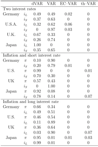
Table 7 gives the average percentage weights allotted to each of the four models across 40 samples t = 1 , . . . , n − k , with k = 1 , . . . , 40, i.e. for those samples that were used in the prediction experiments above. From inspecting

18

the sample cases separately, it appears that the method prefers border solu- tions, with two or even three of the models being assigned zero weights. This is due to the fact that the minimization procedure wishes to allot negative weights to some models, which however is excluded by assumption.

The general impression is one of a preference for the two simplest models, the dVAR and the VAR model. There is no recognizable pattern in the relative weights for either of these two models. Positive weights for the linear and nonlinear error-correction structures are rare and isolated.

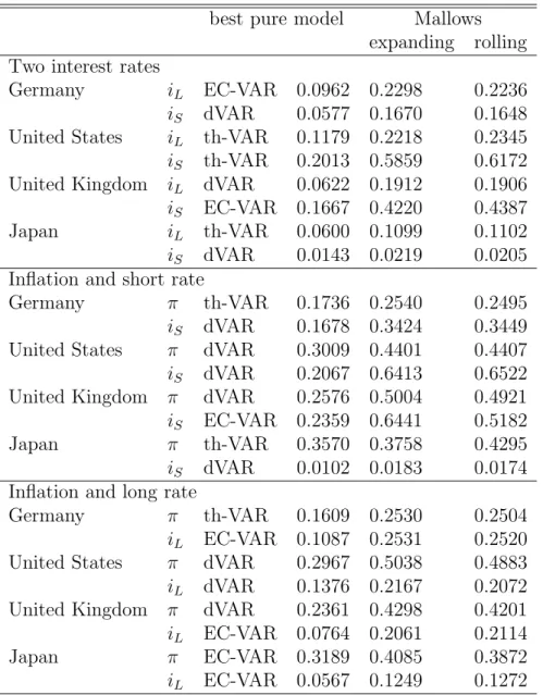
It pays to contrast this in-sample evidence with the prediction horse race of Section 3. The MSE implied by using the ‘optimal’ weights according to the Mallows-criterion optimization are given in Table 8. These values are never smaller than the minimum of the pure-model forecasts, and typically they are considerably worse. We note two extreme cases as examples.

Table 7 shows that the dVAR gets an average weight of 0 for the U.K.

short rate in the ( π, i

) system, while VAR gets a weight of one. By contrast, a comparison with Table 3 shows that the implied Mallows-weight forecast, which necessarily coincides with the pure VAR forecast, is the worst among all pure-model candidates. In a comparable system for the U.S., dVAR and VAR obtain varying weights. The implied forecast, however, is worse than both the pure VAR or pure dVAR forecasts. This indicates that the weights may optimize some in-sample fit but they certainly fail to optimize prediction.

Table 9 repeats the analysis of Table 7 for a slightly different experimental design. Instead of using the data points t = 1 , . . . , n − k to predict the observations at n − k + 1, we now use a data window of fixed size. This design takes care of the argument that structures may change slowly, such that this rolling forecast may outperform the increasing-sample forecast, as it forgets outdated information.

It turns out that, firstly, the results do not change too much with re- spect to model weights. The simple models dVAR and VAR obtain the largest weights, and instances of substantial contributions by EC–VAR and the-VAR are rare. Furthermore, there are no consistent gains in prediction accuracy, as can be seen from comparing the last two columns of Table 8.

The rolling design wins in 14 out of 24 cases, the difference to the expected 12 is insignificant. This indicates that our reported findings are not sensitive to the type of slow structural change that may be present in the data.

Just like statistical in-sample hypothesis tests, the model averaging anal- ysis is unable to provide a clear and reliable guideline on the best model in the sense of prediction performance. The noteworthy merits of complex models, such as the threshold model, for prediction remain undetected by in-sample statistics. This may be partly due to the traditional measurement of model complexity by the parameter dimension. Alternative concepts for

19

Table 7: Average weights for models over the evaluation range for expanding windows.

dVAR VAR EC–VAR th–VAR

Two interest rates

Germany i

0.49 0.49 0.02 0

i

0.37 0.63 0 0

U.S.A. i

0.32 0.62 0.06 0

i

0 0.97 0.03 0

U.K. i

0.67 0.33 0 0

i

0.26 0.74 0 0

Japan i

1.00 0 0 0

i

0.35 0.65 0 0

Inflation and short interest rate

Germany π 0.10 0.90 0 0

i

0.20 0.79 0.01 0

U.S. π 0.99 0 0 0.01

i

0.70 0.30 0 0

UK π 0.57 0.43 0 0

i

0 1.00 0 0

Japan π 0.92 0.08 0 0

i

0.78 0.14 0 0.07

Inflation and long interest rate

Germany π 0.66 0.34 0 0

i

0.49 0.51 0 0

U.S. π 0.46 0.54 0 0

i

0.11 0.89 0 0

UK π 0.36 0.64 0 0

i

0.03 0.90 0 0.07

Japan π 0.95 0.01 0.01 0.03

i

0.99 0.01 0 0

20

Table 8: MSE for single-step prediction.

best pure model Mallows expanding rolling Two interest rates

Germany i

EC-VAR 0.0962 0.2298 0.2236 i

dVAR 0.0577 0.1670 0.1648 United States i

th-VAR 0.1179 0.2218 0.2345 i

th-VAR 0.2013 0.5859 0.6172 United Kingdom i

dVAR 0.0622 0.1912 0.1906 i

EC-VAR 0.1667 0.4220 0.4387

Japan i

th-VAR 0.0600 0.1099 0.1102

i

dVAR 0.0143 0.0219 0.0205 Inflation and short rate

Germany π th-VAR 0.1736 0.2540 0.2495

i

dVAR 0.1678 0.3424 0.3449 United States π dVAR 0.3009 0.4401 0.4407 i

dVAR 0.2067 0.6413 0.6522 United Kingdom π dVAR 0.2576 0.5004 0.4921 i

EC-VAR 0.2359 0.6441 0.5182

Japan π th-VAR 0.3570 0.3758 0.4295

i

dVAR 0.0102 0.0183 0.0174 Inflation and long rate

Germany π th-VAR 0.1609 0.2530 0.2504

i

EC-VAR 0.1087 0.2531 0.2520 United States π dVAR 0.2967 0.5038 0.4883 i

dVAR 0.1376 0.2167 0.2072 United Kingdom π dVAR 0.2361 0.4298 0.4201 i

EC-VAR 0.0764 0.2061 0.2114

Japan π EC-VAR 0.3189 0.4085 0.3872

i

EC-VAR 0.0567 0.1249 0.1272

21

measuring complexity in model selection were developed, for example, by Rissanen (2007). Those ideas have not yet been adapted to the task of model averaging, however.

In order to obtain further insight on the role of the penalty function of the Mallows criterion, we re-ran the averaging search without any penalty.

While this version may appear to allot a weight of one to the most profligate structure, this is not necessarily so because of the AIC lag-order determi- nation. In fact, the non-penalized variant allots slightly larger weights to the VAR and th-VAR models, indeed the most heavily parameterized can- didates. Conversely, imposing a stronger penalty on parameter dimension tends to support the dVAR model but it also wipes the th-VAR model off the map.

Our experiments suggest that in-sample information criteria may be an insufficient device to mimic out-of-sample predictive accuracy. Indeed, un- reported experiments with determining the weights over a training range on the basis of local MSE performance yield weights corresponding to Table 3 and MSE gains relative to Table 8. Because these experiments do not yield further information concerning or main objective, we do not give details here.

6 Summary and conclusion

In a nutshell, our general impression is that the simple dVAR model with- out any theory-guided constraints dominates at very short prediction hori- zons. At longer horizons, error-correction modelling on the basis of reversion to a natural real rate according to the Fisher effect and to an equilibrium yield spread deserves consideration, while the simple dVAR still yields the most robust performance. By contrast, the visually impressive feature of the boundedness of all variables under consideration does not assist in improving prediction. A simple VAR that tends to view all variables as stationary fails, and a sophisticated threshold VAR is unable to convince, showing some ad- vantages at short horizons for some cases but failing for other examples and at longer horizons, when the nonlinearity of the model requires averaging over stochastic predictions.

A ‘threshold’ modification of the linear model that allows variables to behave differently in the distributional tails apparently generates plausible longer-run trajectories, as it is globally stable and avoids the notorious feature of integrated variables that their support is unbounded. The model performs well in some cases for single-step prediction but this dominance remains episodic. The bootstrap validation indicates that it may be risky to rely on the model as a forecasting device.

22

Table 9: Average weights for models over the evaluation range for rolling windows.

dVAR VAR EC–VAR th–VAR

Two interest rates

Germany i

0.71 0.28 0 0.01

i

0.42 0.58 0 0

U.S.A. i

0.17 0.79 0.04 0

i

0 0.98 0.02 0

U.K. i

0.86 0.13 0 0.01

i

0.48 0.46 0.03 0.03

Japan i

0.88 0.12 0 0

i

0.26 0.67 0.06 0.01

Inflation and short interest rate

Germany π 0.59 0.35 0.05 0.02

i

0.51 0.41 0.05 0.04

U.S. π 0.96 0.04 0 0

i

0.71 0.29 0 0

UK π 0.47 0.52 0.01 0

i

0.56 0.44 0 0

Japan π 0.93 0.06 0 0.01

i

0.93 0.05 0 0.02

Inflation and long interest rate

Germany π 0.62 0.37 0.01 0

i

0.46 0.52 0 0.02

U.S. π 0.32 0.68 0 0

i

0.06 0.94 0 0

UK π 0.42 0.58 0 0

i

0.09 0.87 0 0.05

Japan π 0.57 0.39 0.04 0

i

0.88 0.10 0.02 0

23

Ultimately, our model-averaging experiment responds to a recurrent argu- ment that combinations of models may outperform pure predictions ( Bates and Granger , 1969). However, it is difficult to find optimal weights for this aim. We rely on a procedure that has been advocated for classical spec- ification searches in regression models. The implied combined forecast rarely dominates the best pure predictions.

References

[1] Armstrong, J.S. (2007) ‘Significance tests harm progress in forecast- ing,’ International Journal of Forecasting 23, 321–327.

[2] Balke, N.S., and T.B. Fomby (1997) ‘Threshold Cointegration’ In- ternational Economic Review 38, 627–645.

[3] Bates, J., and Granger, C. W. J. (1969). ‘The combination of forecasts,’ Operations Research Quarterly 20, 451–468.

[4] Campbell, J.Y., and Shiller, R.J. (1987) ‘Cointegration and Tests of Present Value Models’ Journal of Political Economy 95, 1062–1088.

[5] Clements, M.P., and Hendry, D.F. (1999) Forecasting Non- Stationary Economic Time Series. Cambridge University Press.

[6] Dickey, D.A., and Fuller, W. (1979) ‘Distribution of the Estima- tors for Autoregressive Time Series with a Unit Root,’ Journal of the American Statistical Association 74(366), 427–431.

[7] Diebold, F.X., and Mariano, R.S. (1995) ‘Comparing Predictive Accuracy,’ Journal of Business and Economic Statistics 13, 253–263.

[8] Engle, R.F., and Granger, C.W.J. (1987) ‘Co-integration and Er- ror Correction: Representation, Estimation and Testing,’ Econometrica 56, 1333–1354.

[9] Engle, R.F., and Yoo, B.S. (1987) ‘Forecasting and Testing in Co- integrated Systems’. Journal of Econometrics 35, 143–159.

[10] de Gooijer, J.G., and Vidiella-i-Anguera, A. (2004) ‘Forecast- ing threshold cointegrated systems,’ International Journal of Forecasting 20, 237–254.

[11] Granger, C.W.J. (2005). ‘Modeling, Evaluation, and Methodology in the New Century’, Economic Inquiry, 43, 1–12.

24

[12] Hall, A.D., Anderson, H.M., and C.W.J. Granger (1992) ‘A Cointegration Analysis of Treasury Bill Yields’ Review of Economics and Statistics 74, 116–126.

[13] Hansen, B. (2007) ‘Least squares model averaging,’ Econometrica 75, 1175–1189.

[14] Hjort, N.L., and G. Claeskens (2003) ‘Frequentist model average estimators,’ Journal of the American Statistical Association 98, 879–

899.

[15] Johansen, S. (1995) Likelihood-Based Inference in Cointegrated Vector Autoregressive Models. Oxford University Press.

[16] Jumah, A., and Kunst, R.M. (2008) ‘Seasonal Prediction of Euro- pean Cereal Prices: Good Forecasts Using Bad Models?,’ Journal of Forecasting 27, 391–406.

[17] Kunst, R.M. (2008) ‘Cross validation of prediction models for seasonal time series by parametric bootstrapping,’ Austrian Journal of Statistics 37, 271–284.

[18] Liebscher, E. (2005) ‘Towards a unified approac for proving geometric ergodicity and mixing properties of nonlinear autoregressive processes,’

Journal of Time Series Analysis 26, 669–689.

[19] Malliaropulos , D. (2000) ‘A note on nonstationarity, structural breaks, and the Fisher effect,’ Journal of Banking and Finance 24, 695–

707.

[20] Mallows, C.L. (1973) ‘Some comments on C

,’ Technometrics 15, 661–675.

[21] Rahbek, A., and Shephard, N. (2002) ‘Inference and Ergodicity in the Autoregressive Conditional Root Model,’ Working paper, University of Copenhagen.

[22] Rissanen , J. (2007) Information and Complexity in Statistical Model- ing. Springer.

[23] Tong, H. (1990. Non-linear time series: a dynamical system approach.

Oxford University Press.

25

Authors: Adusei Jumah, Robert M. Kunst

Title: Optimizing Time-series Forecasts for Inflation and Interest Rates Using Simulation and Model Averaging

Reihe Ökonomie / Economics Series 231

Editor: Robert M. Kunst (Econometrics)

Associate Editors: Walter Fisher (Macroeconomics), Klaus Ritzberger (Microeconomics)

ISSN: 1605-7996

© 2008 by the Department of Economics and Finance, Institute for Advanced Studies (IHS),

Stumpergasse 56, A-1060 Vienna • +43 1 59991-0 • Fax +43 1 59991-555 • http://www.ihs.ac.at

ISSN: 1605-7996