Growth Regressions, Principal Components and Frequentist Model Averaging

IHS Economics Series Working Paper 236

March 2009

Growth Regressions, Principal Components and Frequentist Model Averaging

Martin Wagner

Jaroslava Hlouskova

Impressum Author(s):

Martin Wagner, Jaroslava Hlouskova Title:

Growth Regressions, Principal Components and Frequentist Model Averaging ISSN: Unspecified

2009 Institut für Höhere Studien - Institute for Advanced Studies (IHS) Josefstädter Straße 39, A-1080 Wien

E-Mail: o ce@ihs.ac.atffi Web: ww w .ihs.ac. a t

All IHS Working Papers are available online: http://irihs. ihs. ac.at/view/ihs_series/

This paper is available for download without charge at:

https://irihs.ihs.ac.at/id/eprint/1907/

Growth Regressions, Principal Components and Frequentist Model Averaging

Martin Wagner, Jaroslava Hlouskova

236

Reihe Ökonomie

Economics Series

236 Reihe Ökonomie Economics Series

Growth Regressions, Principal Components and Frequentist Model Averaging

Martin Wagner, Jaroslava Hlouskova March 2009

Institut für Höhere Studien (IHS), Wien

Institute for Advanced Studies, Vienna

Contact:

Martin Wagner

Department of Economics and Finance Institute for Advanced Studies Stumpergasse 56

1060 Vienna, Austria : +43/1/599 91-150 email: mawagner@ihs.ac.at

Jaroslava Hlouskova

Department of Economics and Finance Institute for Advanced Studies Stumpergasse 56

1060 Vienna, Austria : +43/1/599 91-142 email: hlouskov@ihs.ac.at

Founded in 1963 by two prominent Austrians living in exile – the sociologist Paul F. Lazarsfeld and the economist Oskar Morgenstern – with the financial support from the Ford Foundation, the Austrian Federal Ministry of Education and the City of Vienna, the Institute for Advanced Studies (IHS) is the first institution for postgraduate education and research in economics and the social sciences in Austria.

The Economics Series presents research done at the Department of Economics and Finance and aims to share “work in progress” in a timely way before formal publication. As usual, authors bear full responsibility for the content of their contributions.

Das Institut für Höhere Studien (IHS) wurde im Jahr 1963 von zwei prominenten Exilösterreichern – dem Soziologen Paul F. Lazarsfeld und dem Ökonomen Oskar Morgenstern – mit Hilfe der Ford- Stiftung, des Österreichischen Bundesministeriums für Unterricht und der Stadt Wien gegründet und ist somit die erste nachuniversitäre Lehr- und Forschungsstätte für die Sozial- und Wirtschafts- wissenschaften in Österreich. Die Reihe Ökonomie bietet Einblick in die Forschungsarbeit der Abteilung für Ökonomie und Finanzwirtschaft und verfolgt das Ziel, abteilungsinterne Diskussionsbeiträge einer breiteren fachinternen Öffentlichkeit zugänglich zu machen. Die inhaltliche Verantwortung für die veröffentlichten Beiträge liegt bei den Autoren und Autorinnen.

Abstract

This paper offers two innovations for empirical growth research. First, the paper discusses principal components augmented regressions to take into account all available information in well-behaved regressions. Second, the paper proposes a frequentist model averaging framework as an alternative to Bayesian model averaging approaches. The proposed methodology is applied to three data sets, including the Sala-i-Martin et al. (2004) and Fernandez et al. (2001) data as well as a data set of the European Union member states' regions. Key economic variables are found to be significantly related to economic growth.

The findings highlight the relevance of the proposed methodology for empirical economic growth research.

Keywords

Frequentist model averaging, growth regressions, principal components

JEL Classification

C31, C52, O11, O18, O47

Comments

Financial support from the Jubiläumsfonds of the Oesterreichische Nationalbank (Project number:

11688) is gratefully acknowledged. The regional data set has been compiled and made available to us by Robert Stehrer from the Vienna Institute for International Economic Studies (WIIW). The comments of seminar participants at Universitat Pompeu Fabra, Barcelona, are gratefully acknowledged. The usual disclaimer applies.

Contents

1 Introduction 1

2 Description of the Econometric Approach 5

3 Empirical Analysis 11

3.1 Sala-i-Martin, Doppelhofer and Miller Data ... 11 3.2 Fernandez, Ley and Steel Data ... 19 3.3 European Regional Data ... 24

4 Summary and Conclusions 27

References 29 Appendix A: Description of Regional Data Set 32

Appendix B: Additional Empirical Results 35

Appendix C: Inference for Model Average Coefficients 37

1 Introduction

This paper offers a twofold contribution to the empirical growth literature. First, it advocates the use of well-behaved principal components augmented regressions (PCAR) to capture and condition on the relevant information in the typically large set of variables available.

Second, it proposes frequentist model averaging as an alternative to Bayesian model averaging approaches commonly used in the growth regressions literature. Model averaging, Bayesian or frequentist, becomes computationally cheap when combined with principal components augmentation.

The empirical analysis of economic growth is one of the areas of economics in which progress seems to be hardest to achieve (see e.g. Durlauf et al., 2005) and where few definite results are established. Large sets of potentially relevant candidate variables have been used in empirical analysis to capture what Brock and Durlauf (2001) refer to as theory open endedness of economic growth, and numerous econometric techniques have been used to separate the wheat from the chaff. Sala-i-Martin (1997b) runs two million regressions and uses a modification of the extreme bounds test of Leamer (1985), used in the growth context earlier also by Levine and Renelt (1992), to single out what he calls ‘significant’ variables. Fernandez et al.

(2001) and Sala-i-Martin et al. (2004) use Bayesian model averaging techniques to identify important growth determinants. Doing so necessitates the estimation of a large number of potentially ill-behaved regressions (e.g. in case of near multi-collinearity of the potentially many included regressors) or regressions which suffer from omitted variables biases in case important explanatory variables are not included. Hendry and Krolzig (2004) use, similar to Hoover and Perez (2004), a general-to-specific modelling strategy to cope with the large amount of regressors while avoiding the estimation of a large number of equations. Clearly, also in a general-to-specific analysis a certain number of regressions, typically greater than one, has to be estimated.

In a situation in which the potential relevance of large sets of variables is unclear ex ante,

any regression including only few explanatory variables is potentially suffering from large

biases in case that some or many relevant explanatory variables have been excluded from the

regression. However, with the large numbers of variables available it is often infeasible or even

impossible to include all variables in the regression. As an example, for one of the data sets

employed in this paper, originally used in Sala-i-Martin et al. (2004), the reciprocal condition

number of the full regressor matrix including all available explanatory variables is 9.38×10

. Thus, in the full regression not only is there a very small number of degrees of freedom left, but the coefficients are estimated with additional imprecision due to the numerical (almost) singularity. Consequently, a trade-off has to be made between parsimony of the regression (to achieve low variance but potentially high bias) and the inclusion of as many potentially relevant variables as possible (to achieve low bias at the price of potentially high variance).

In many applications it is conceivable that the researcher has a set of variables in mind whose effect she wants to study in particular. This choice of variables can e.g. be motivated by a specific theoretical model or also by the quest of understanding the contribution to growth of certain factors like human capital related variables. In such a situation, conditional upon an ex ante classification in core and auxiliary variables, the use of principal components augmented regressions allows to focus on untangling the effect of the core variables on growth whilst controlling for by conditioning on the effects of the auxiliary variables. Performing regression analysis including the core variables and principal components computed from the auxiliary variables allows to take into account ‘most’ of the information contained in all variables. In particular including principal components of the auxiliary variables in addition to the core variables implies that the bias of the resulting regression will be low, since ‘most’ of the information contained in all available variables is taken into account (see the discussion below in Section 2). Also, a PCAR typically does not suffer from large estimation variance when the number of core variables and (mutually orthogonal) principal components is reasonably small and multi-collinearity is absent.

The coefficients to the core variables in a PCAR measure the effect on growth of each of these variables when considered jointly whilst in addition conditioning out the information contained in the principal components and are in this sense

‘robust’ estimates.

The fact that in a PCAR most of the information of all variables is included, potentially mitigates the necessity to account for model uncertainty via model averaging. Clearly, how- ever, PCAR analysis can be combined with model averaging, either Bayesian or frequentist (classical). Given the separation in core and auxiliary variables, a natural approach to model averaging is to compute sub-models only with respect to the core variables, whilst including the principal components in all regressions. This has several advantages: First, including

1As long as the set of core variables are not multi-collinear, multi-collinearity can be controlled by choosing the number of included principal components accordingly.

in each regression the principal components minimizes potential (omitted variables) biases compared to regressions including only small numbers of variables. Up to now in empirical growth analysis model averaging has been performed mainly over small models, e.g. in the Bayesian model averaging approach pursued in Sala-i-Martin et al. (2004) the mean prior model size is 7 for most of the discussion. This may result in the presence of substantial bi- ases. Second, resorting to PCAR reduces the number of sub-models enormously. If one were to estimate all sub-models (in case all of them can be estimated) for all k variables, then 2

regressions are necessary, which amounts to 2

regressions for the Sala-i-Martin et al. (2004) data and 2

regressions for the Fernandez et al. (2001) data also considered in this paper.

Clearly, these numbers are way too large to estimate all sub-model regressions. The Bayesian literature tries to overcome this limitation by resorting to MCMC sampling schemes designed to approximate the posterior densities of all coefficients. The posteriors depend by defini- tion upon the priors, where as mentioned, large weights are typically put on small models with potentially large biases. In PCAR analysis, the number of regressions to be computed to estimate all sub-models is reduced from 2

to 2

, where k

denotes the number of core variables, which typically (at least in our applications) is a rather small number that allows for the estimation of all sub-models. For a Bayesian approach this implies that the posterior distributions can be evaluated exactly, be it analytically or numerically. Furthermore, each of the estimated sub-model PCARs has comparably small omitted variables bias due to the inclusion of principal components.

In this paper we perform model averaging in a frequentist framework, using recent advantages in the statistics literature which allow to perform valid classical inference in a model averaging context, see in particular Claeskens and Hjort (2008) and the brief description in Appendix C.

In our analysis we consider four different weighting schemes. One, as a benchmark, uses equal

weights for each model and the three others are based on weights derived from information

criteria computed for the individual models. These are Mallows model averaging (MMA)

advocated by Hansen (2007), and smoothed AIC and smoothed BIC weights considered by

Buckland et al. (1997) and studied in detail also in Claeskens and Hjort (2008). Furthermore,

we introduce frequentist analogs to quantities considered to be informative in a Bayesian

model averaging framework. E.g. we introduce, for any given weighting scheme, the so-called

inclusion weight as the classical counterpart of the Bayesian posterior inclusion probability of

a variable. Similarly, we consider the distribution of model weights over model sizes.

We apply the methodology to three data sets, with two of them taken from widely cited papers. The first data set is that of Sala-i-Martin et al. (2004), containing 67 explanatory variables for 88 countries. The second one is the Fernandez et al. (2001) data set, based in turn on data used in Sala-i-Martin (1997b), which contains 41 explanatory variables for 72 countries. The third data set comprises the 255 NUTS2 regions of the 27 member states of the European union and contains 48 explanatory variables. These data sets have also been analyzed in Schneider and Wagner (2008), who use the adaptive LASSO estimator of Zou (2006), to perform at the same time model (i.e. variable) selection and parameter estimation.

For the two well studied data sets, the sets of variables selected in Schneider and Wagner (2008) correspond closely to the sets of variables found important (measured by posterior inclusion probabilities) in the original papers. To illustrate the PCAR and frequentist model averaging (FMA) approaches advocated in this paper we consider for each of the three data sets the variables selected in Schneider and Wagner (2008) as core variables and all remaining variables as auxiliary variables. The main finding is that our approach singles out, both when considering single PCAR estimates as well as model average estimates, core economic variables as important in explaining economic growth. E.g. for the Sala-i-Martin et al. (2004) data these are initial GDP, primary education and the investment price. Furthermore, the coefficient to initial GDP is about twice as large compared to Sala-i-Martin et al. (2004) and hence the conditional β-convergence speed (see e.g. Barro, 1991) is about twice as high as found in Sala- i-Martin et al. (2004). Several dummy, political and other variables, most notably the East Asian dummy having highest posterior inclusion probability in Sala-i-Martin et al. (2004), are not significant. Qualitatively similar findings prevail also for the Fernandez et al. (2001) data. For the European regional data in particular human capital appears to be significantly related to growth. Our findings show the importance of appropriate conditioning, via inclusion of principal components of the large set of potential explanatory variables, in uncovering the variables important to explain economic growth. From a computational perspective it turns out that the specific choice of information criterion based weighting scheme has limited importance on the model averaging results. This holds true especially for the inclusion weight ranking of variables but to a large extent also for the estimated model average coefficients.

The paper is organized as follows. Section 2 describes the econometric methods used. Sec-

tion 3 contains the empirical analysis and results and Section 4 briefly summarizes and con-

cludes. Three appendices follow the main text. Appendix A briefly describes the European

regional data, Appendix B collects some additional empirical results and Appendix C de- scribes the computation of confidence intervals for frequentist model average coefficients.

2 Description of the Econometric Approach

Let y ∈ R

denote the variable to be explained (in our application average per capita GDP growth for N countries respectively regions) and collect all explanatory variables in X = [X

X

] ∈ R

, with the core variables given in X

∈ R

and the auxiliary variables in X

∈ R

with k = k

+ k

. Without loss of generality we assume that all variables have zero mean, since in all growth regressions an intercept is typically included. As is well known, by the Frisch-Waugh theorem, the regression can equivalently be estimated with demeaned variables. The regression including all variables is given by

y = X

β

+ X

β

+ u. (1)

The information for regression (1) contained in X

is equivalently summarized in the set of (orthogonal) principal components corresponding to X

, i.e. in the set of transformed variables ˘ X

= X

O, with O ∈ R

computed from the eigenvalue decomposition of Σ

= X

X

(due to the assumption of zero means):

Σ

= X

X

= OΛO

= [O

O

]

· Λ

0 0 Λ

¸ · O

O

¸

= O

Λ

O

+ O

Λ

O

, (2)

where O

O = OO

= I

and Λ = diag(λ

, . . . , λ

), λ

≥ λ

for i = 1, . . . , k

− 1. The partitioning into variables with subscripts 1 and 2 will become clear in the discussion below.

From (2) the orthogonality of ˘ X

is immediate, since ˘ X

X ˘

= Λ.

Let us consider the case of multi-collinearity in X

first (which e.g. necessarily occurs when

k

> N) and let us denote the rank of X

with r. Take Λ

∈ R

, hence Λ

= 0 and

X

X

= O

Λ

O

. The space spanned by the columns of X

∈ R

coincides with the

space spanned by the orthogonal regressors ˜ X

= X

O

∈ R

, i.e. with the space spanned

by the r principal components. Thus, in this case regression (1) is equivalent to the regression

y = X

β

+ ˜ X

β ˜

+ u (3)

in the sense that both regressions lead to exactly the same fitted values and residuals. Fur-

thermore, in case [X

X ˜

] has full rank, regression (3) leads to unique coefficient estimates

of β

and ˜ β

. Since linear regression corresponds geometrically to a projection this is evident and of course well known.

Resorting to principal components, however, also has a clear interpretation and motivation in case of full rank of X

and hence of Σ

. In such a situation replacing X

by the first r principal components ˜ X

leads to a regression where the set of regressors ˜ X

spans that r- dimensional subspace of the space spanned by the columns of X

such that the approximation error to the full space is minimized in a least squares sense. More formally the following holds true, resorting here to the population level.

Let x

∈ R

be a mean zero random vector with covariance matrix Σ

(using here the same notation for both the sample and the population quantity for simplicity). Consider a decomposition of x

in a factor component and a noise component, i.e. a decomposition x

= Lf + ν, with f ∈ R

, L ∈ R

and ν ∈ R

(for a given value of r). If the decomposition is such that the factors f and the noise ν are uncorrelated, then Σ

= LΣ

L

+Σ

. Principal components analysis performs an orthogonal decomposition of x

into Lf and ν such that the noise component is as small as possible, i.e.

it minimizes E(ν

ν ) = tr(Σ

). As is well known, the solution is given by f = O

x

, L = O

, with O

∈ R

and ν = O

O

x

, using the same notation for the spectral decomposition as above.

Therefore, including only r principal components ˜ X

instead of all regressors X

has a clear interpretation. The principal components augmented regression (PCAR) includes ‘as much information as possible’ (in least squares sense) with r linearly independent regressors con- tained in the space spanned by the columns of X

. We write the PCAR as:

y = X

β

+ ˜ X

β ˜

+ ˜ u, (4) neglecting in the notation the dependence upon the (chosen) number of principal components r but indicating with ˜ u the difference of the residuals to the residuals of (3). Including only the information contained in the first r principal components of X

in the regression when the rank of X

is larger than r of course amounts to neglecting some information and hence leads to different, larger residuals. Thus, in comparison to the full regression (1), if it can be estimated, the PCAR regression will in general incur some bias in the estimates which has to be weighed against the benefits of a lower estimator variance. It is immediate that the choice of r is a key issue. The larger r, the more information is included but the fewer degrees of

2I.e. we now consider thek2-dimensional random vectorx2 for whichX2, a sample of sizeN, is available.

freedoms are left (i.e. a lower bias but a higher variance) and multi-collinearity (since the λ

are ordered decreasing in size) may become a problem.

Any choice concerning r is based on the eigenvalues λ

, where ‘large’ eigenvalues are typically attributed to the factors and

‘small’ ones to the noise. The literature provides many choices in this respect and we have experimented with several thereof.

A classical, descriptive approach is given by the so-called variance proportion criterion (VPC),

r

= min

j=1,...,k2

à j|

P

i=1

λ

P

i=1

λ

≥ 1 − α

!

, (5)

with α ∈ [0, 1]. Thus, r

is the smallest number of principal components such that a fraction 1−α of the variance is explained. For our applications setting α = 0.2, i.e. explaining 80% of the variance, leads to reasonable numbers of principal components included. In the context of growth regressions there is no underlying theoretical factor model explaining the second-moment structure of the auxiliary variables X

available, thus any choice has to a certain extent a heuristic character and has to trade off good approximation (necessary to capture the information contained in all explanatory variables for small bias) with a suffi- ciently small number of principal components (necessary for well-behaved regression analysis with low variance).

When computing the principal components from the regressors X

∈ R

in our growth application, we split this set of variables in two groups. One group contains the quantitative or cardinal variables and the other includes the dummy or qualitative variables. We separate these two groups to take into account their different nature when computing principal com- ponents. For both groups the principal components are computed based on the correlation matrix of the variables. Computing the principal components based on the correlation matrix is especially important for the group of quantitative variables. These differ considerably in magnitude, due to their scaling which we keep unchanged for the Fernandez et al. (2001) and Sala-i-Martin et al. (2004) data to use exactly the same data as in these papers. Computing the principal components based on the covariance matrix leads in such a case to essentially fitting the ‘large’ variables, whereas the computation based on the correlation matrix corrects

3Note here that multi-collinearity cannot only appear within ˜X2 but in the joint regressor matrix [X1X˜2].

In any empirical application this can, however, be easily verified and if necessary remedied by removing some variables from the set of orthogonal regressors ˜X2in order to have a well-behaved PCAR.

4In addition to the results reported in the paper the number of principal components has been determined using the testing approaches of Lawley and Maxwell (1963), Malinowski (1989), Faber and Kowalski (1997), Schott (2006) and Kritchman and Nadler (2008). In a variety of simulations, however, the VPC criterion and a simple eigenvalue test based on the correlation matrix (see below) have performed best.

for scaling differences and leads to a scale-free computation of the principal components. To be precise, a weighted principal components problem is solved in which the function to be minimized is given by E(ν

Qν) = tr(QΣ

) with Q = diag(σ

, . . . , σ

2,k2

), neglecting here for simplicity the separation of the variables in X

in quantitative and dummy variables.

This leads to f = O

Q

x

, L = Q

O

and ν = Q

O

O

Q

x

, i.e. the auxiliary regressors are given by ˜ X

= X

Q

O

.

For a chosen number of principal components, the PCAR (4) allows to estimate the conditional effects of the variables X

taking into account the relevant information contained in X

and summarized in ˜ X

. As discussed in the introduction, one can also use (4) as a starting point to consider model averaging. By resorting to PCAR analysis, the number of regressions to be computed to estimate all sub-models is reduced from 2

to 2

if one computes all sub- models with respect to the core variables. The number of regressions can be reduced further by partitioning the set of variables X

= [X

X

], with X

∈ R

included in each regression and X

∈ R

, where k

= k

+ k

, contains the variables in- or excluded in the sub-models estimated. This further reduces the number of regressions to be computed to 2

and makes it even more likely that all sub-models can be estimated. As already mentioned in the introduction, the small number of models has the advantage, for both classical and Bayesian approaches that inference need not be based on estimation results obtained only on subsets of the model space with a focus on small models.

We denote the sub-model regressions, based on the partitioning of (4) as

y = X

β

(j) + X

(j)β

(j) + ˜ X

β ˜

(j) + ˜ u(j). (6) The sub-models M

are indexed with j = 1, . . . , 2

, where X

(j) denotes subset j of X

. The corresponding coefficient estimates are given by ˆ β(j) = [ ˆ β

(j)

β ˆ

(j)

β ˜

(j)

]

∈ R

. Here, with some imprecision in notation we include in ˆ β

(j) ∈ R

zero entries corresponding to all variables not included in model M

, whereas in (4) the dimension of β

(j) equals the number of variables of X

included. We are confident that this does

5Performing the spectral decomposition on a correlation matrix allows for another simple descriptive crite- rion concerning the number of principal components. By construction the trace of a correlation matrix equals its dimensions, i.e. is equal tok2. Therefore, if allk2 eigenvalues were equally large, they all would equal 1.

This suggests to include as many principal components as there are eigenvalues larger than 1, i.e. to consider the eigenvalues larger than 1 as big and those smaller than 1 as small. The results correspond closely to those obtained with VPCαwithα= 0.2.

6This statement has to be interpreted correctly: Inference is based on a different type of subset of the model space, since all information contained inX2 is summarized in ˜X2 and taken into account. This conditional model space, after purging the effects of ˜X2, however, is then fully exhausted.

not lead to any confusion.

Furthermore, note already here that the regression including all explanatory variables, i.e. all variables in X

, will be referred to as full model in the empirical application. Model average coefficients ˆ β

are computed as weighted averages of the coefficient estimates of the sub-regressions, i.e.

β ˆ

=

2^k12

X

j=1

w(j) ˆ β(j), (7)

with 0 ≤ w(j) ≤ 1 and P

j=1

w(j) = 1. We consider four different weighting schemes:

equal weights, MMA weights as considered in Hansen (2007) and smoothed AIC (S-AIC) and smoothed BIC (S-BIC) weights considered by Buckland et al. (1997) and discussed in detail in Claeskens and Hjort (2008). Equal weighting assigns weights w(j) =

to each of the models. By definition, this model averaging scheme does not allocate model weights according to any measure of quality of the individual models and thus serves more as a baseline averaging scheme. The other model averaging schemes base the model weights on different information criteria to give higher weights to models showing better performance in the ‘metric’ of the underlying information criterion. Hansen (2007), based on Li (1987), advocates the use of a Mallows criterion for model averaging that under certain assumptions results in optimal model averaging in terms of minimal squared error of the corresponding model average estimator amongst all model average estimators. The MMA model weights are obtained by solving a quadratic optimization problem. Denote with ˆ U = [ˆ u(1), . . . , u(2 ˆ

)] ∈ R

the collection of residual vectors of all models and with M = [dim(M

), . . . , dim(M

)]

∈ R

the dimensions of all models. The dimension of M

is given by k

+r plus the number of variables of X

included in M

. Further, denote with ˆ σ

the estimated residual variance from the full model including all variables of X

. Then, the MMA weight vector is obtained by solving the following quadratic optimization problem, where w = [w(1), . . . , w(2

)]

∈ R

is the vector of weights corresponding to all models.

min

n

w

U ˆ

U w ˆ + 2ˆ σ

w

M o

(8) subject to: w ≥ 0,

2^k12

X

j=1

w(j) = 1.

7Note furthermore that we can, since ˜X2are included in each regression, invoke the Frisch-Waugh theorem and entirely equivalently consider model averaging only for the regressions of y onX11 and the subsets of X12 by considering the residuals of the regressions of y,X11 and X12 on ˜X2. This equivalent interpretation highlights again that the inclusion of ˜X2 conditions on the ‘relevant’ information contained inX2.

The remaining two averaging schemes base their weights on the information criteria AIC and BIC, defined here as AIC(j) = N ln ˆ σ

+ 2dim(M

) and BIC (j) = N ln ˆ σ

+ ln N dim(M

), where ˆ σ

is the estimated residual variance of M

. Based on these the corresponding model weights are computed as w(j) = exp{−

AIC(j)}/ P

m

exp{−

AIC(m)} for S-AIC weights and as w(j) = exp{−

BIC(j)}/ P

m

exp{−

BIC(m)} for S-BIC weights.

Each of the variables in X

is included in exactly half of the models considered. The model average coefficient corresponding to each of the variables X

, i = 1, . . . , k

can be written as

β ˆ

=

2

X

j=1

w(j) ˆ β

(j) (9)

= X

j:X12,i∈M/ j

w(j)0 + X

j:X12,i∈Mj

w(j) ˆ β

(j).

This shows the shrinkage character of model averaging. This is most clearly seen for equal weighting, for which the inclusion weight of variable i, i.e. P

j:X12,i∈Mj

w(j), is exactly 1/2 for all variables X

. Hence for equal weighting the average coefficient is given by

times the sum of all coefficient estimates over only 2

(i.e. half of the) models. More generally, for any given weighting scheme the inclusion weight of variable i indicates the importance of this particular variable, in the ‘metric’ of the chosen weighting scheme. Thus, the inclusion weight is in a certain sense the classical alternative to Bayesian posterior inclusion probabilities. If the inclusion weight of a certain variable is high, this means that the 50% of the models in which this variable is included have a high explanatory power or good performance for e.g.

with respect to AIC or BIC.

Given model average coefficients proper inference concerning them, e.g. to test for significance,

is important. Correct statistical inference has to take into account that model averaging

estimators are (random) mixtures of correlated estimators. Frequentist (or classical) inference

taking these aspects into account has been developed in Hjort and Claeskens (2003) and is

discussed at length in Claeskens and Hjort (2008, Chapter 7). A brief description of the

computational aspects is contained in Appendix C and for further conceptual considerations

we refer the reader to the cited original literature.

3 Empirical Analysis

As mentioned in the introduction, the empirical analysis is performed for three different data sets. These are the data sets used in Sala-i-Martin et al. (2004), in Fernandez et al. (2001) and a data set covering the 255 NUTS2 regions of the 27 member states of the European Union.

In the discussion below we retain the variable names from the data files we received from Gernot Doppelhofer for the Sala-i-Martin et al. (2004) data and also use the original names used in the file downloaded from the homepage of the Journal of Applied Econometrics for the Fernandez et al. (2001) data to facilitate the comparison with the results in these papers.

The selection of core and auxiliary variables considered in this paper is based on the results obtained with the same data sets in Schneider and Wagner (2008). That paper follows a complementary approach to growth regressions in terms of obtaining point estimates of the coefficients to the relevant variables by resorting to adaptive LASSO estimation (see Zou, 2006). This estimation procedure performs at the same time consistent parameter estimation and model selection. We include (all respectively a subset of) the variables found important in that paper in our set X

. For the Sala-i-Martin et al. (2004) and Fernandez et al. (2001) data sets the sets of variables found important in Schneider and Wagner (2008) are very similar to the sets of variables found important in the original papers based on Bayesian model averaging techniques, see the discussion in the respective subsections below. Thus, the sets X

include for these two data sets variables found to be important by studies using very different methods and thus constitute a potentially relevant starting point for applying the approach outlined in the previous section. Note that the choice of variables to be included in X

is here based on statistical analysis rather than being motivated by a particular economic theory model or question. By definition the results obtained with our approach depend upon the allocation of variables in the sets X

and X

. Consequently, this is a key issue that deserves attention and our allocation based on the statistical analysis performed in Schneider and Wagner (2008) implies that the analysis performed and the results reported in this paper have to a certain extent illustrative character.

3.1 Sala-i-Martin, Doppelhofer and Miller Data

The data set considered in Sala-i-Martin et al. (2004) contains 67 explanatory variables for 88

countries. The variables and their sources are described in detail in Table 1 in Sala-i-Martin

et al. (2004, p. 820–821). The dependent variable is the average annual growth rate of real

per capita GDP over the period 1960–1996.

As core variables (i.e. as regressors X

) we consider 12 out of the 67 explanatory variables of the data set. In the list of variables to follow we include whether the estimated coefficients, the point estimates in Schneider and Wagner (2008, Table 2) and the posterior means of Sala-i-Martin et al. (2004, Table 4, p. 830), are positive or negative. The signs of the point estimates and the posterior means coincide for all variables. Furthermore we also include the rank with respect to posterior inclusion probability as given in Sala-i-Martin et al. (2004, Table 3, p. 828–829). Given that the largest part of the discussion in Sala-i-Martin et al.

(2004) is for the results based on priors with mean model size 7 we compare our results throughout with these results of Sala-i-Martin et al. (2004). The variables are in alphabetical order of abbreviation: BUDDHA (fraction of population Buddhist in 1960, positive, 16), CONFUC (fraction of population Confucian in 1960, positive, 9), EAST (East Asian dummy, positive, 1), GDP (log per capita GDP in 1960, negative, 4), GVR61 (share of expenditure on government consumption of GDP in 1961, negative, 18), IPRICE (investment price, negative, 3), LAAM (Latin American dummy, negative, 11), MALFAL (index of malaria prevalence in 1966, negative, 7), P (primary school enrollment rate, positive, 2), REVCOUP (number of revolutions and coups, negative, 41), SAFRICA (sub-Saharan Africa dummy, negative, 10), TROPICAR (fraction of country’s land in tropical area, negative, 5).

We consider 3 out of the 12 variables to be included in all regressions, i.e. X

= [EAST GDP P].

The East Asian dummy and the primary school enrollment rate are the two variables with the highest inclusion probabilities in Sala-i-Martin et al. (2004). Initial GDP is also found to be important and is by definition the central variable in the conditional β -convergence literature. Thus, in total only 2

= 512 regressions are estimated for this data set. The total computation time is just a few minutes on a standard PC, showing that from a computational point of view also all 2

= 8 × 512 = 4096 sub-model regressions could be estimated. The computationally most intensive part is actually the solution of the quadratic optimization problem to obtain the MMA weights. Out of the 55 variables in X

, 11 are dummy variables (see Appendix B). Using the VPC criterion with 80%, 13 principal components are included

8In Schneider and Wagner (2008) 14 variables are selected by the adaptive LASSO algorithm. However, the coefficients for two of them are not significant, with standard errors computed as described in Zou (2006), in the final equation and have therefore been not included in X1. These are GDE (average share of public expenditure on defense, positive, 45) and GEEREC (average share of public expenditure on education, positive, 48). As can be seen also their ranks with respect to posterior inclusion probability are rather high. Hence, these two variables are included inX2.

−0.0050 0 0.005 0.01 0.015 0.02 0.025 20

40 60 80 100 120

EAST

−0.01250 −0.012 −0.0115 −0.011 −0.0105 −0.01 −0.0095 −0.009 −0.0085 −0.008

100 200 300 400 500 600 700

GDP

0.0180 0.02 0.022 0.024 0.026 0.028 0.03

50 100 150 200 250 300

P

0.0060 0.008 0.01 0.012 0.014 0.016 0.018 0.02 0.022

20 40 60 80 100 120 140 160 180

BUDDHA

0.010 0.015 0.02 0.025 0.03 0.035 0.04 0.045 0.05

10 20 30 40 50 60 70

CONFUC

−0.060 −0.05 −0.04 −0.03 −0.02 −0.01 0

5 10 15 20 25 30 35 40 45

GVR61

−9 −8.5 −8 −7.5 −7 −6.5 −6 −5.5 −5 −4.5

x 10⁻⁵ 0

1 2 3 4 5 6 7

8x 10⁴ IPRICE

−0.020 −0.015 −0.01 −0.005 0 0.005 0.01

10 20 30 40 50 60 70 80 90

LAAM

−0.0160 −0.014 −0.012 −0.01 −0.008 −0.006 −0.004 −0.002 0

20 40 60 80 100 120 140 160

MALFAL

−14 −12 −10 −8 −6 −4 −2 0 2

x 10⁻³ 0

50 100 150 200

250 REVCOUP

−14 −12 −10 −8 −6 −4 −2 0 2 4

x 10⁻³ 0

20 40 60 80 100 120 140 160

180 SAFRICA

−0.0180 −0.016 −0.014 −0.012 −0.01 −0.008 −0.006

50 100 150 200 250

TROPICAR

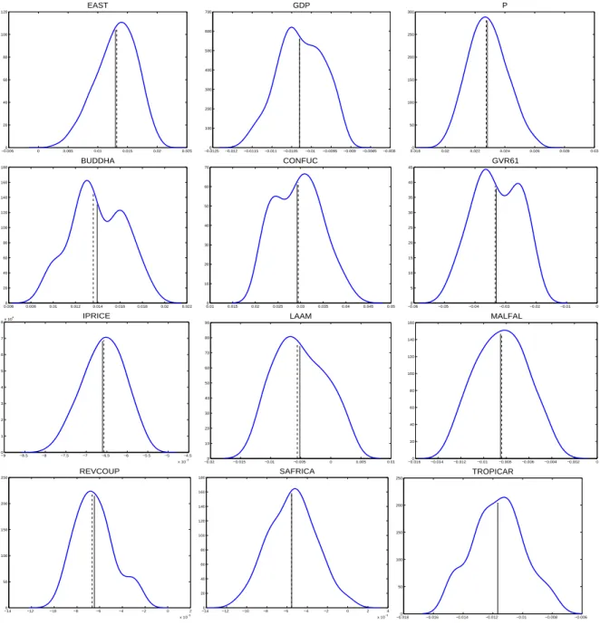
Figure 1: Empirical coefficient densities over all estimated models where the respective vari-

ables are included for the Sala-i-Martin et al. (2004) data set. The solid vertical lines display

the means and the dashed vertical lines display the medians.

for the 44 quantitative variables and 6 principal components for the 11 dummy variables.

Thus, in total 19 variables are included in ˜ X

. Together, with 12 variables in X

the full regression includes 31 variables.

The smallest regression includes 22 variables, the three variables in X

and the 19 principal components.

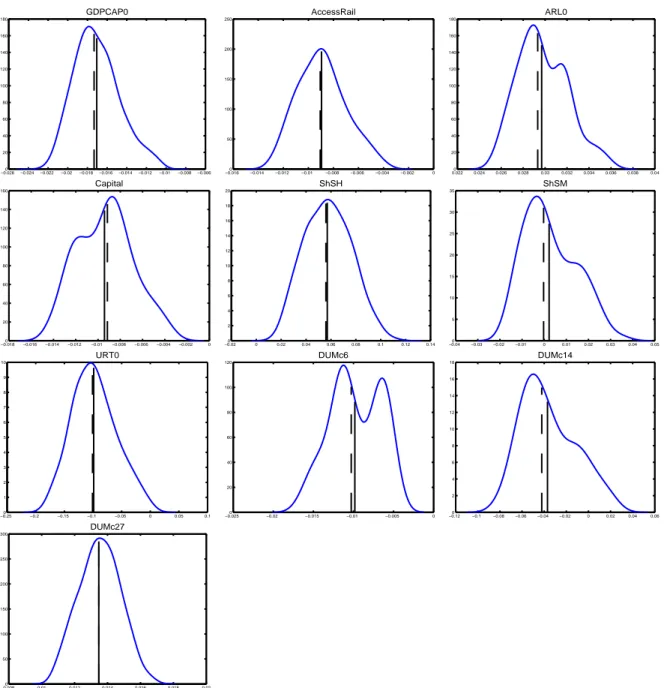
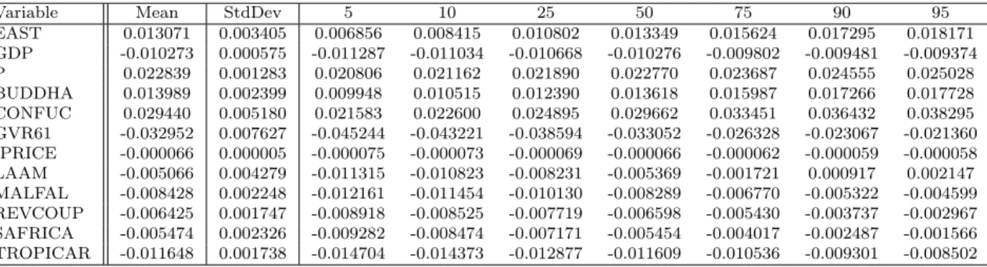
Figure 1 displays the empirical coefficient densities for the coefficients to the variables in X

, ordered (alphabetically within groups) as first those in X

and then those in X

. All empirical coefficient densities displayed in this paper are based on Gaussian kernels with the bandwidths chosen according to Silverman’s rule of thumb, see Silverman (1986) for details.

For all coefficients to variables in X

the densities are computed based on all 2

available estimates, and for the coefficients to variables in X

the densities are, of course, based on only the 2

estimates in the models where the respective variables are included. Numerical information (mean, standard deviation and quantiles) concerning these empirical distributions is contained in table format in Table 9 in Appendix B. For some of the variables (BUDDHA, CONFUC, GVR61) bimodality occurs over the set of models estimated. It is important to note that these densities cannot be interpreted in a similar fashion as posterior densities in a Bayesian framework. The empirical densities merely visualize the variability of the estimated coefficients over all estimated models. These individual coefficients are then weighted with several weighting schemes to obtain model average coefficients. It is the unknown densities of the model average coefficients that are the classical counterparts to posterior densities.

The means displayed in Figure 1 correspond by construction to the model average estimates for the equal weights weighting scheme for the coefficients to the variables in X

and are twice the means for the coefficients to the variables in X

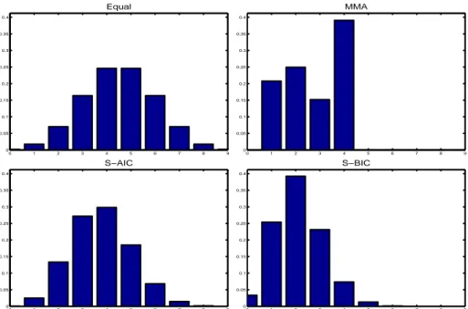
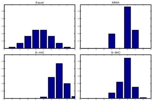
when the means are computed over all models, i.e. not conditional upon inclusion. Figure 2 displays the distribution of model weights over the model sizes for the four discussed model averaging schemes, see also Table 10 in Appendix B. This figure, as well as the similar ones for the other two data sets, displays for simplicity the model size ranging from 0 to dim(X

), i.e. 1 (for the intercept) plus the number of variables in X

and the number of principal components included are not added on the horizontal axis. The ‘real’ model sizes are 1 + k

+ r = 23 (i.e. the intercept, the variables X

and the principal components) plus the numbers indicated in the figure.

9Using 31 explanatory variables, or 32 if the intercept (i.e. the demeaning) is counted as well, for 88 observations could be seen as too large a number. The number of variables can be reduced by explaining a smaller percentage than 80% of the variance of the auxiliary variables or by computing the principal components from all 55 variables together. We have experimented with both possibilities and have found that the results are very robust.

0 1 2 3 4 5 6 7 8 9 0

0.05 0.1 0.15 0.2 0.25 0.3 0.35 0.4

Equal

0 1 2 3 4 5 6 7 8 9

0 0.05 0.1 0.15 0.2 0.25 0.3 0.35 0.4

MMA

0 1 2 3 4 5 6 7 8 9

0 0.05 0.1 0.15 0.2 0.25 0.3 0.35 0.4

S−AIC

0 1 2 3 4 5 6 7 8 9

0 0.05 0.1 0.15 0.2 0.25 0.3 0.35 0.4

S−BIC

Figure 2: Distribution of model weights over model sizes for the Sala-i-Martin et al. (2004) data set. The weighting schemes displayed are: Equal (upper left graph), MMA (upper right graph), S-AIC (lower left graph) and S-BIC (lower right graph).

Alternatively, the numbers in the figure are the model sizes in the second regression, using again the Frisch-Waugh interpretation, after demeaning all variables and after conditioning on the information contained in ˜ X

. For valid inference the real model size needs to be considered. By construction, the upper left graph simply displays the corresponding binomial weights but the other graphs are more informative. E.g. MMA averaging allocates all weights to model sizes ranging from 1 to 4 with 39% allocated to models with 4 variables included.

The lower two graphs, corresponding to S-AIC and S-BIC model averaging, display that as expected S-BIC weighting allocates more weight on smaller models than S-AIC weighting.

The model size with largest weight is 4 (30%) for S-AIC and 2 (39%) for S-BIC.

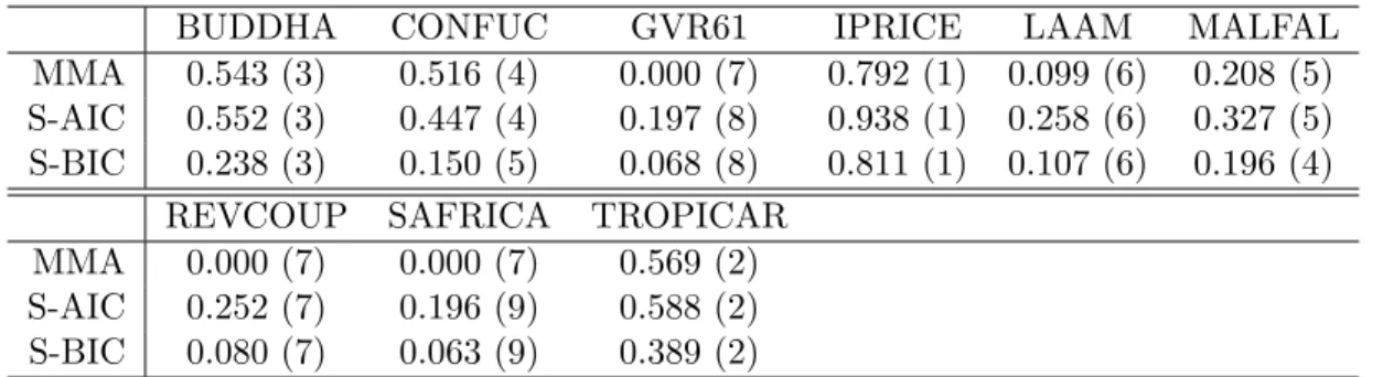
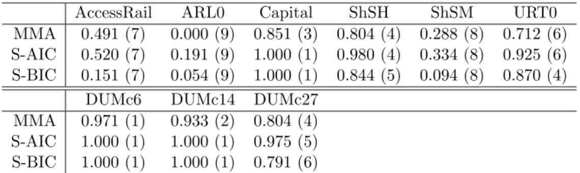
Table 1 displays the inclusion weights for the 9 variables in X

. Two observations can be

made. First, the numerical values of the inclusion weights differ across the three weighting

schemes but the rankings almost perfectly coincide. The highest inclusion weight is obtained

for IPRICE and is, depending upon weighting scheme, between 79% for MMA weights and

94% for S-AIC weights. The lowest inclusion weights are 0 for MMA weights for the variables

GVR61, REVCOUP and SAFRICA. Second, the rankings differ from the ranking of these

variables according to posterior inclusion probabilities in Sala-i-Martin et al. (2004). For

BUDDHA CONFUC GVR61 IPRICE LAAM MALFAL MMA 0.543 (3) 0.516 (4) 0.000 (7) 0.792 (1) 0.099 (6) 0.208 (5) S-AIC 0.552 (3) 0.447 (4) 0.197 (8) 0.938 (1) 0.258 (6) 0.327 (5) S-BIC 0.238 (3) 0.150 (5) 0.068 (8) 0.811 (1) 0.107 (6) 0.196 (4)

REVCOUP SAFRICA TROPICAR

MMA 0.000 (7) 0.000 (7) 0.569 (2) S-AIC 0.252 (7) 0.196 (9) 0.588 (2) S-BIC 0.080 (7) 0.063 (9) 0.389 (2)

Table 1: Inclusion weights and ranks in brackets for the variables that are in- respectively excluded in model averaging for the three data dependent model averaging schemes for the Sala-i-Martin et al. (2004) data.

about half of the variables the same ranking as in Sala-i-Martin et al. (2004) (when ranking only these 9 variables) is found, namely for CONFUC (for MMA and S-AIC), GVR61 (for S- AIC and S-BIC), IPRICE, LAAM and TROPICAR. Note for completeness that the posterior inclusion probabilities of Sala-i-Martin et al. (2004) are for most variables relatively similar to the numbers reported in Table 1, in particular to the inclusions weights obtained with MMA or S-BIC weights, indicating that at the outset quite different approaches lead to rather similar results with respect to the importance of the inclusion of certain variables.

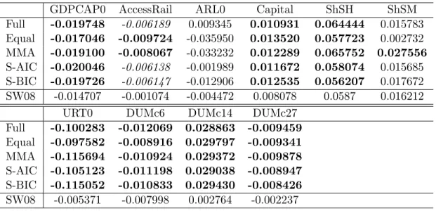
The next question addressed is now the contribution of the individual variables in terms of their coefficients. The estimation results for the full regression and the model average coefficients are displayed in Table 2. Significance for the full equation estimates is computed using OLS standard errors. For the model average coefficients inference is performed as developed in Claeskens and Hjort (2008) and as described briefly in the previous section and in Appendix C. Both in the full equation as well as for the model average coefficients only few variables are significant. In the full equation these are log per capita GDP in 1960 (GDP), the primary school enrollment rate (P) and the investment price (IPRICE). Furthermore two religion variables, the fraction of Buddhist in the population in 1960 (BUDDHA) and the fraction of Confucian in the population in 1960 (CONFUC), are significant at the 10%

level in the full equation. When considering model average coefficients only GDP, P and

IPRICE are significant, with the latter being significant only at the 10% level when using

equal weights. Thus, only three key economic variables are found to be significantly related

to economic growth when including the information contained in the auxiliary variables by

including principal components. Note that the significance of variables is highly related to

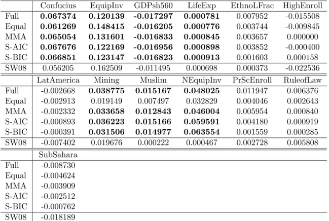
EAST GDP P BUDDHA CONFUC GVR61 Full 0.006681 -0.010399 0.021586 0.015432 0.036302 -0.032472 Equal 0.013071 -0.010273 0.022839 0.006994 0.014720 -0.016476 MMA 0.012274 -0.010362 0.023435 0.009770 0.016824 0.000000 S-AIC 0.012248 -0.010556 0.023508 0.008714 0.013572 -0.004972 S-BIC 0.014706 -0.010672 0.024268 0.003625 0.004117 -0.001787 SDM04 0.017946 -0.005849 0.021374 0.002340 0.011212 -0.004594 SW08 0.013874 -0.001452 0.016097 0.012027 0.025531 -0.041727

IPRICE LAAM MALFAL REVCOUP SAFRICA TROPICAR

Full -0.000066 -0.005742 -0.004173 -0.008964 -0.006988 -0.008287 Equal -0.000033 -0.002533 -0.004214 -0.003212 -0.002737 -0.005824 MMA -0.000054 -0.001078 -0.002521 -0.000000 -0.000000 -0.006852 S-AIC -0.000062 -0.001925 -0.002445 -0.001682 -0.000863 -0.006821 S-BIC -0.000054 -0.000873 -0.001826 -0.000481 -0.000246 -0.004844 SDM04 -0.000065 -0.001901 -0.003957 -0.000205 -0.002265 -0.008308 SW08 -0.000071 -0.002593 -0.001841 -0.002174 -0.002010 -0.005398 Table 2: Coefficient estimates for the Sala-i-Martin et al. (2004) data. Full displays the coef- ficient estimates corresponding to the full model; Equal the estimates corresponding to equal model weights; MMA the estimates using the weights as discussed in Hansen (2007); S-AIC the estimates computed with smoothed AIC weights and S-BIC the estimates computed with smoothed BIC weights. Bold typesetting indicates significance at the 5% significance level and italic numbers indicate significance at the 10% level, computed as discussed in Claeskens and Hjort (2008).

The rows labelled SDM04 display the unconditional posterior means of the coefficient esti- mates computed from Sala-i-Martin et al. (2004, Table 3, p. 828–829) and Sala-i-Martin et al. (2004, Table 4, p. 830) for mean prior model size 7. The rows labelled SW08 display the adaptive LASSO point estimates of Schneider and Wagner (2008, Table 2).

the inclusion weights, since amongst the variables in X

the variable IPRICE has the highest inclusion weight.

How do these findings relate to those in Sala-i-Martin et al. (2004)? Considering again model average coefficients, the three variables with significant coefficients are highly ranked in terms of posterior inclusion probability in Sala-i-Martin et al. (2004): GDP (4), P (2) and IPRICE (3). A key difference is that the variable with the highest inclusion probability, the East Asian dummy is not found to be significantly related to economic growth.

Also several other political, religious or health variables found to be important in Sala-i-Martin et al. (2004) are not significant in our results. Furthermore, the β-convergence speed implied by

10In supplementary material, available upon request, we provide for all three data sets also the model average estimates conditional upon inclusion.

11To be precise, the corresponding model average coefficient is significant at the 10% level for both equal and S-BIC weights.