Precipitation and temperature drive continental-scale patterns in stream invertebrate production

(1)

E C O L O G Y

Precipitation and temperature drive continental-scale patterns in stream invertebrate production

C. J. Patrick¹*, D. J. McGarvey², J. H. Larson³, W. F. Cross⁴, D. C. Allen⁵, A. C. Benke⁶, T. Brey⁷, A. D. Huryn⁶, J. Jones⁸, C. A. Murphy⁹, C. Ruffing¹⁰, P. Saffarinia¹¹,

M. R. Whiles¹², J. B. Wallace¹³, G. Woodward¹⁴

Secondary production, the growth of new heterotrophic biomass, is a key process in aquatic and terrestrial eco- systems that has been carefully measured in many flowing water ecosystems. We combine structural equation modeling with the first worldwide dataset on annual secondary production of stream invertebrate communities to reveal core pathways linking air temperature and precipitation to secondary production. In the United States, where the most extensive set of secondary production estimates and covariate data were available, we show that precipitation-mediated, low–stream flow events have a strong negative effect on secondary production. At larger scales (United States, Europe, Central America, and Pacific), we demonstrate the significance of a positive two- step pathway from air to water temperature to increasing secondary production. Our results provide insights into the potential effects of climate change on secondary production and demonstrate a modeling framework that can be applied across ecosystems.

INTRODUCTION

Secondary production is the generation of new heterotrophic biomass over time. It is a fundamental ecosystem process because it requires the consumption of basal energetic sources while sustaining consumers at higher trophic levels in both aquatic and terrestrial food webs (1–5).

Secondary production can be used to assess higher- level responses to environmental change (6) and human perturbations (7, 8), including ecosystem services such as water filtration (9, 10) and fisheries produc- tion (11, 12). Understanding how secondary production may respond to climate change is therefore essential. Invertebrates are diverse and productive members of most food webs and comprise the majority of metazoan diversity globally. Previous research has characterized local- scale effects of temperature on individual invertebrate taxa (13–15), but the potential effects of continental- to global-scale shifts in temperature and precipitation on entire communities of invertebrate sec- ondary producers are largely unknown (16).

Identifying drivers of annual community secondary production (ACSP), defined as the sum of annual production of all invertebrate populations within a community (17), is particularly challenging because individual- and species-level processes do not always scale up to the community level in a direct additive manner. Functional

redundancy in the roles that species play within a food web can offset environmental perturbations via compensatory effects on overall production (18). For this reason, ACSP may be a more useful holistic indicator of the ecosystem-level effects of climate change than production rates of discrete taxa or functional groups. Unfortunately, studies of the effects of macroscale shifts in temperature and precipitation on ACSP, which are difficult to conduct in experimental settings, are rare [but see (19)].

Previous research in stream and river ecosystems provides a unique opportunity to further understand the linkages between ACSP and climate. When compared to other types of ecosystems, empirical studies of ACSP in streams and rivers are relatively common (20, 21).

We leveraged this previous work by combining a literature review on freshwater ACSP with geospatial analysis, hydrologic modeling, and structural equation modeling (SEM) to test hypotheses linking air temperature and precipitation to ACSP in lotic ecosystems. Our ultimate goal was to build a systems-level framework that can be expanded or refined in future research and used to predict climate- driven changes in ACSP.

Our study focuses primarily on the effects of air temperature and precipitation on ACSP because both factors are closely linked to physicochemical conditions in freshwater ecosystems. Air tempera- ture is a principal driver of water temperature in lotic systems (22), and water temperature stimulates in-stream primary production (23, 24); this two-step pathway may link air temperature to ACSP (25). Precipitation effects on ACSP may be mediated by hydrology, which is a key determinant of habitat stability for benthic invertebrates that reside on or within streambed substrates. Stable flows promote well-sorted substrates that support high invertebrate den- sities and allow extended growth periods (26, 27). In contrast, systems that experience extreme floods and/or droughts tend to have low secondary production (7, 28, 29).

We began this study with an extensive literature review of empirical measurements of ACSP in lotic ecosystems and associated in situ covariates, such as water temperature and channel substrate characteristics. We then used a geographic information system to append spatially derived covariates, including land use, elevation,

1Department of Life Sciences, Texas A&M University, 6300 Ocean Drive, Corpus Christi, TX 78412, USA. ²Center for Environmental Studies, Virginia Commonwealth University, Richmond, VA 23284, USA. ³Upper Midwest Environmental Sciences Center, U.S. Geological Survey, 2630 Fanta Reed Rd., La Crosse, WI 54603, USA. ⁴Depart- ment of Ecology, Montana State University, Bozeman, MT 59717, USA. ⁵Depart- ment of Biology, University of Oklahoma, 730 Van Vleet Oval, Norman, OK 73019, USA. ⁶University of Alabama, Tuscaloosa, AL 35487, USA. ⁷Alfred Wegener Institute, Helmholtz Center for Polar and Marine Research, Bremerhaven & Helmholtz Institute for Functional Marine Biodiversity at the University of Oldenburg, Oldenburg, Germany.

8University of Alaska Fairbanks, Fairbanks, AK 99775, USA. ⁹Department of Fisheries and Wildlife, Oregon State University, Corvallis, OR 97331, USA. ¹⁰University of British Columbia, 2329 West Mall, Vancouver, BC V6T 1Z4, Canada. ¹¹University of California, Riverside, 900 University Ave., Riverside, CA 92521, USA. ¹²Department of Zoology, Cooperative Wildlife Research Laboratory and Center for Ecology, Southern Illinois University, Carbondale, IL 62901, USA. ¹³Department of Entomology and Odum School of Ecology, University of Georgia, Athens, GA 30602, USA.

14Department of Life Sciences, Imperial College London, Silwood Park Campus, Buckhurst Rd., Ascot, Berkshire SL5 7PY, UK.

*Corresponding author. Email: christopher.patrick@tamucc.edu

exclusive licensee American Association for the Advancement of Science. No claim to original U.S. Government Works. Distributed under a Creative Commons Attribution NonCommercial License 4.0 (CC BY-NC).

on April 17, 2019http://advances.sciencemag.org/Downloaded from

(2)

slope, and local climate, to the ACSP data. Many environmental covariates were available for study sites within the United States, but only climate and elevation data were consistently available for sites outside of the United States. New hydrologic variables, such as minimum 30-day stream flow (the minimum average discharge that persists for 30 consecutive days), were then calculated by using ex- isting covariates as predictors in statistical models (see Materials and Methods) and appended to the covariate data for U.S. sites. By combining covariates from multiple sources, we were able to ex- pand the number of variables and causal pathways that we tested in models of ACSP.

Links between climate and ACSP were then tested with a combi- nation of traditional univariate regression analysis and SEM. The latter approach was central to our study because SEMs can be used to evaluate cause-and-effect relationships among discrete variables (30), can explicitly account for covariation among variables, and can simultaneously test systems-level hypotheses that are expressed as complex networks of interrelationships among variables (31). Devel- opment of SEMs of ACSP constitutes a significant advance, relative to previous reviews of aquatic secondary production (1, 32), because it allows us to evaluate multiple drivers of ACSP within a single inte- grative framework. In addition, this study demonstrates a novel yet general approach to integrate meta-analysis of published results, covariate data that were mined from independent sources and appended to published data, and statistical modeling (univariate regression and SEM) for the purpose of deriving greater insight from published information and creating new conceptual understanding of connections among suites of environmental and biotic variables.

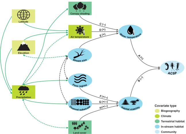
Before model building and testing, we outlined an a priori hy- pothesis or “metamodel” (30) of systems-level links between major climate variables and ACSP (Fig. 1). Habitat stability and water temperature were predicted to be proximal drivers of ACSP. Hy- drology (28), channel substrate (33), and land cover (34) were pre- dicted to drive habitat stability. Air temperature (22), canopy shading (35), and stream channel size (36) were predicted to influence water temperature. Precipitation, latitude, and elevation were predicted to act as distal effects on ACSP, mediated through their effects on temperature and riparian vegetation.

Models were tested at two distinct spatial scales. First, we modeled ACSP at the continental scale, using only U.S. study sites. This allowed us to test complex cause-and-effect relationships using the full suite of environmental covariates that was assembled for U.S. sites. Sec- ond, we developed simpler ACSP models at a larger scale that included sites from Europe, Central and South America, and New Zealand.

These inclusive models were constrained by the smaller number of environmental covariates that were available at all study sites, but they did allow us to test the generality of some key results from the U.S. models.

RESULTS AND DISCUSSION

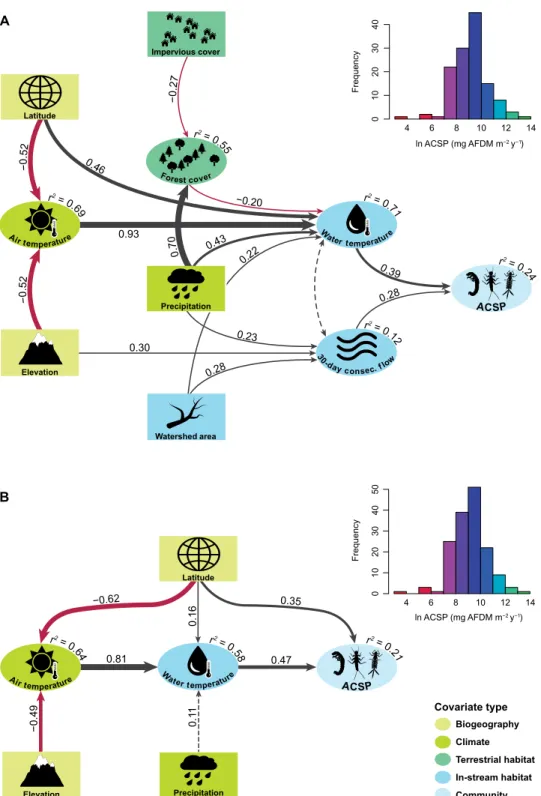
Among all U.S. samples, ACSP spanned four orders of magnitude [35 to 612,231 mg ash-free dry mass (AFDM) m⁻² year⁻¹] and was strongly positively skewed [median, 9991; coefficient of variation (CV), 0.41; see Fig. 2A, inset]. A nearly identical distribution of ACSP was observed at the global scale (median, 9982; CV, 0.42; see Fig. 2B, inset). In U.S. streams, univariate regression analyses detected significant positive effects of mean annual water temperature, basin area, minimum 30-day flow, and percent urban development on

ACSP (Table 1), consistent with hypothesized links A, B, E, F, and H in Fig. 1. A significant negative effect was also detected for percent forest cover, as predicted by link C in the metamodel. Of the univariate relationships, water temperature had the strongest overall effect on ACSP (standardized effect size  = 0.39).

Nine covariates and 14 path links were retained in the final SEM for U.S. streams (Fig. 2A and Table 2). Of these, some paths were simple and predictable, such as the strong effect of air temperature on water temperature (37), the effects of latitude and elevation on air temperature, and the effect of precipitation on minimum 30-day discharge. However, other paths were more complex. For instance, the total effect of precipitation on water temperature included two paths: a direct positive link from precipitation to water temperature and a negative indirect link that was mediated by forest cover (precipitation → forest cover → water temperature; see Fig. 2A).

This indirect effect of precipitation on water temperature may be attributed to wetter regions having comparatively dense forests with larger canopies and more extensive shading (38, 39) or enhanced evaporation (40).

The U.S. SEM confirmed many of the hypothesized pathways in the metamodel (Fig. 1), most notably the direct influence of base flow stability and water temperature on ACSP. Significant indirect effects of climate (air temperature and precipitation), the physical landscape (catchment elevation and basin area), and land cover (impervious surface area and forest cover) on ACSP were mediated through their direct effects on water temperature and base flow stability. The final inclusive SEM complimented the U.S. model by confirming that air temperature and precipitation have consistent, predictable effects on ACSP that are mediated by their direct effects on water temperature (Fig. 2B).

The positive effect of water temperature on ACSP in the U.S. and global models is perhaps intuitive, but our quantitative results raise pressing theoretical questions and can help to reconcile conflicting results from previous site-specific studies. The metabolic theory of ecology (MTE) predicts that standing stock biomass should de- crease with increasing temperature, while the production-to-biomass (P:B) relationship should increase with temperature, resulting in no net change in secondary production (41). Some empirical support for this prediction is provided by observational meta-analyses (32) and controlled in situ stream warming experiments (16), but other studies have documented net positive effects of temperature on body size, growth rates, and total production (1, 25). Our results, which constitute the most comprehensive meta-analysis to date, indicate that the relationship between temperature and ACSP is net positive.

Given that the MTE assumes constant resource supply, we posit that the mechanism responsible for the observed positive relationship between water temperature and ACSP may be a temperature-mediated increase in basal resources (42). Thus, we suggest that closer exam- ination of the effect of basal resources on ACSP should be a priority area in future research (43–45).

Basal resources are likely to improve systems-level models of ACSP because food quality and quantity are already known to be fundamental determinants of individual growth (46–48) and of ACSP (49) in aquatic ecosystems. For instance, allochthonous leaf litter has low nutritional value, relative to autochthonous material, but can account for >90% of the annual variation in secondary produc- tion within temperate streams because it is so abundant (45, 50, 51).

Allochthonous material was not included in our models because it was not measured at most study sites (see data file 2). However,

(3)

using a subset of U.S. studies that measured both allochthonous organic material and ACSP (n = 41), we detected a strong positive univariate relationship between coarse particulate organic matter (CPOM) and ACSP (r² = 0.279, P < 0.001). Notably, CPOM accounted for more of the variation in ACSP than water temperature and habitat stability combined (in the U.S. SEM; see Fig. 2A). We are therefore confident that additional information on basal resources and the mechanisms that link them to climate (52–55) will enhance our abil- ity to predict ACSP in changing climates.

Hydrology also stood out as a key regulator of ACSP. Results from U.S. streams indicated that discharge magnitude during dry or low flow periods (i.e., minimum 30-day flow) has a significant positive effect ( = 0.24) on ACSP (Fig. 2A and Table 1). While this is consistent with previous site-specific findings that environmental stability increases in-stream production (56–58), our study is the first to demonstrate this relationship at the continental scale. Hy- drologic stability, as one dimension of environmental stability in lotic ecosystems, is known to have a significant effect on secondary production (59–62), particularly in drought-prone systems (63).

However, the effect of hydrology did not extend to measures of flooding or “flashiness.” These factors are important to invertebrates in some lotic ecosystems (26, 58, 64), but they did not have a signif- icant effect on ACSP in our analyses. This may be due to variation

among communities in the response to flashiness, where naturally flashy streams are inhabited by organisms with adaptive traits that convey resilience (59, 65).

One notable difference between the U.S. and inclusive models was a significant positive effect of absolute latitude on ACSP; this link between latitude and ACSP, which was independent of a latitu- dinal effect on temperature, was detected in the inclusive model but not in the final U.S. model. The difference may be an artifact of the truncated range of latitudes among U.S. streams relative to the global range. However, it may also indicate that additional information on benthic community structure is needed to understand ACSP at global scales. Links between benthic diversity, biomass (66, 67), and sec- ondary production (68, 69) have been documented in freshwater ecosystems, and benthic invertebrate diversity is known to vary with latitude (70, 71). Incorporating new dimensions of community struc- ture, such as diversity and standing stock biomass, may therefore help to explain the effect of latitude on ACSP.

Moving forward, an obvious goal should be to increase the explained variation in ACSP. Coefficients of determination for ACSP were <0.25 in both the U.S. and global SEMs (Fig. 2)—a strong indication that some key variables were not included in the models.

Here, our goal was to advance conceptual understanding of the systems- level drivers of ACSP by identifying causal pathways that link climate

A

B C

D E

F G H Canopy shading

Air temperature Latitude

Elevation

Precipitation

Flow regime

Land cover

Biogeography Climate Terrestrial habitat In-stream habitat Community Covariate type

Stream size

Channel substrate Habitat stability

ACSP

Water temperature (-)

(+) (+)

(+/-) (+/-) (+/-)

(+)

(-)

Fig. 1. Conceptual diagram or metamodel of major hypothesized influences on ACSP. Covariates that are external to stream ecosystems (i.e., exogenous variables) are indicated by rectangles. Covariates that are direct measures of in-stream conditions or processes (i.e., endogenous variables) are indicated by ovals. Each covariate is also recognized as one of five color-coded types (see inset key): biogeography, climate, terrestrial habitat, in-stream habitat, and community. Solid black arrows depict known causal effects among covariates. Arrow labels correspond to exemplar references [A (23, 25), B (26, 27), C (35, 94), D (22, 95), E (36, 96), F (7, 28), G (29, 33), H (34, 97)].

Parenthetic signs next to black arrow labels indicate that the relationship is expected to be positive (+), negative (−), or variable (+/−). Solid green arrows depict fundamental relationships that are expected but not explicitly documented here (e.g., the negative relationship between latitude and air temperature). Dashed arrows depict

hypothesized covariation among variables. on April 17, 2019http://advances.sciencemag.org/Downloaded from

(4)

Frequency

4 6 8 10 12 14

010203040

ln ACSP (mg AFDM m⁻² y⁻¹)

Frequency

4 6 8 10 12 14

01020304050

ln ACSP (mg AFDM m⁻² y⁻¹)

−0.52

−0.5

2

0.46

−0.27

−0.20 0.93

700. 0.43

0.30

0.28 0.23

0.22

0.39 0.28

−0.62 0.35

r² = 0.69

r² = 0.55

r² = 0.71

r² = 0.12

r² = 0.24

r² = 0.64

r² = 0.58

r² = 0.21

−0.49 0.11

0.81 0.47

0.16

A

B

Latitude

Latitude Air temperature

Elevation

Watershed area Precipitation Forest cover Impervious cover

Water temperature

30-day consec. flow

ACSP

Air temperature W

ater temperature

ACSP

Elevation Precipitation

Biogeography Climate Terrestrial habitat In-stream habitat Community Covariate type

Fig. 2. SEMs of ACSP in streams and rivers. Models include an SEM for the U.S. (A) and for global streams and rivers (B). Exogenous variables are indicated by rectangles, and endogenous variables are represented by ovals. Coefficients of determination (r²) are shown for all endogenous variables, and standardized path coefficients are shown for all modeled relationships. Positive and negative effects among variables are depicted by black and red arrows, respectively, with arrow widths proportional to effect sizes (i.e., path coefficients). In the U.S. model, significant covariance between mean annual water temperature (“Water temperature”) and the minimum average discharge that persists for 30 consecutive days (“30-day consec. flow”) is depicted by a dashed double-headed arrow. In the global model, the dashed arrow between mean annual precipitation (“Precipitation”) and mean annual water temperature indicates a nominally significant (P = 0.09) effect; all other relationships in the U.S. and global models are significant at P = 0.05. Both the U.S. and global models satisfied each of the three model fit criteria, with significant ² P values (U.S. = 0.06; global = 0.63), standardized root mean squared residuals (U.S. = 0.06; global = 0.02), and comparative fit index values (U.S. = 0.97; global > 0.99). Inset histograms show the distribution of natural log (ln)–transformed ACSP at U.S. and global scales. Covariate types are as shown in Fig. 1.

(5)

to ACSP; we did not seek to maximize explained variation in ACSP per se. The SEM allowed us to test the hypothesized linkages among variables (Fig. 1) in a critical and explicit way. Nevertheless, future progress will benefit from the addition and testing of new covariates and links between climate and ACSP.

Basal resource availability was previously noted as a priority research topic. Another focus area should be the role of anthropogenic stressors on ACSP. Previous research has reported a positive relationship between some land-use activities and ACSP that covaries with watershed area (72). Consistent with this earlier finding, we detected a positive relationship between watershed area and ACSP. However, when impervious surface area and agricultural land use were added to preliminary SEMs, we were unable to detect a significant influence of either variable on ACSP. The apparent lack of a strong land-use effect on ACSP may be a sampling artifact, as many of the study sites were located at field stations where human impacts were likely minimal. For example, 64% of all streams in the U.S. database were entirely unaffected by row-crop agriculture and only 7% of the U.S. streams flowed through watersheds, where row- crop agriculture accounted for >10% of internal land use. Thus, the current ACSP database may be ill suited to evaluate land-use effects, leaving a key information gap to be filled.

Despite the limitations of the ACSP models, our results have clear implications for ecosystem function in the face of climate change.

Climate models predict that over the next century, average air tem- peratures will continue to rise (73) and precipitation patterns will shift markedly (74, 75). Our models suggest that these changes will

have cascading effects on ACSP mediated through water temperature and discharge during dry periods. For instance, the SEMs predict that warming temperatures will tend to increase ACSP. How- ever, the frequency and severity of low flow events are expected to increase in many ecosystems as subhumid regions transition to semiarid climates (75–77). If these systems are populated by in- vertebrates that lack physiological or life history traits that allow them to persist under drought conditions, temperature-driven increases in ACSP are likely to be offset by increased mortality or diminished recruitment.

In conclusion, we suggest that four key areas of research should now be pursued to advance understanding of ACSP. First, new ACSP data from undersampled regions are needed to determine whether the results presented here are applicable in other parts of the globe.

Second, a better understanding of the roles that basal resources or other bottom-up trophic constraints play in regulating ACSP and how these basal factors are affected by climate is needed. Third, the effects of anthropogenic stressors should be incorporated in systems- level models. Fourth, the general ACSP results should be tested using habitat-specific production estimates (3, 60, 62), paying special attention to account for differential effects on specific invertebrate traits or functional groups (78, 79). Addressing each of these needs will be a challenging and labor-intensive process, but we have shown that an enhanced understanding of the complex mechanisms that drive ACSP at continental to global scales is achievable when the efforts and data of many ecologists are integrated within an appro- priate modeling framework.

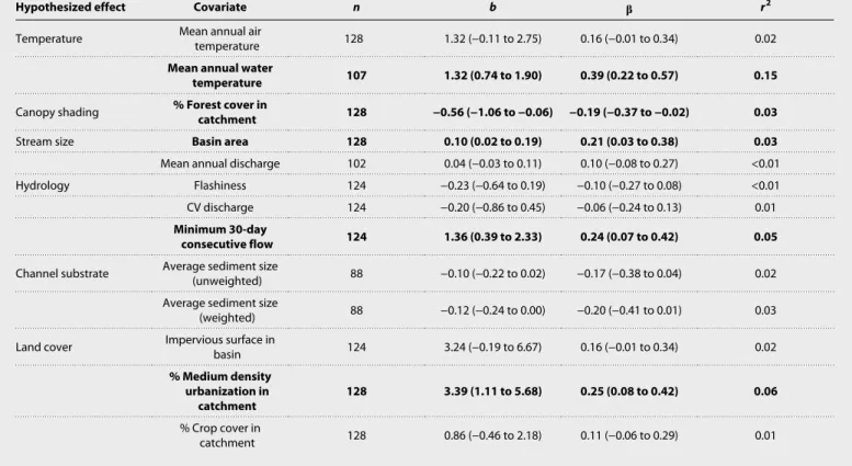
Table 1. Comparison of effect sizes in univariate regression models of ACSP in U.S. streams. Unstandardized regression slopes (b) and standardized slopes () are each reported with 95% confidence intervals (shown in parentheses) as well as sample sizes (n) and coefficients of determination (r²). Covariates shown in bold text have slopes (95% confidence intervals) that exclude zero and are therefore considered statistically significant.

Hypothesized effect Covariate n b  r²

Temperature Mean annual air

temperature 128 1.32 (−0.11 to 2.75) 0.16 (−0.01 to 0.34) 0.02

Mean annual water

temperature 107 1.32 (0.74 to 1.90) 0.39 (0.22 to 0.57) 0.15

Canopy shading % Forest cover in

catchment 128 −0.56 (−1.06 to −0.06) −0.19 (−0.37 to −0.02) 0.03

Stream size Basin area 128 0.10 (0.02 to 0.19) 0.21 (0.03 to 0.38) 0.03

Mean annual discharge 102 0.04 (−0.03 to 0.11) 0.10 (−0.08 to 0.27) <0.01

Hydrology Flashiness 124 −0.23 (−0.64 to 0.19) −0.10 (−0.27 to 0.08) <0.01

CV discharge 124 −0.20 (−0.86 to 0.45) −0.06 (−0.24 to 0.13) 0.01

Minimum 30-day

consecutive flow 124 1.36 (0.39 to 2.33) 0.24 (0.07 to 0.42) 0.05

Channel substrate Average sediment size

(unweighted) 88 −0.10 (−0.22 to 0.02) −0.17 (−0.38 to 0.04) 0.02

Average sediment size

(weighted) 88 −0.12 (−0.24 to 0.00) −0.20 (−0.41 to 0.01) 0.03

Land cover Impervious surface in

basin 124 3.24 (−0.19 to 6.67) 0.16 (−0.01 to 0.34) 0.02

% Medium density urbanization in

catchment 128 3.39 (1.11 to 5.68) 0.25 (0.08 to 0.42) 0.06

% Crop cover in

catchment 128 0.86 (−0.46 to 2.18) 0.11 (−0.06 to 0.29) 0.01

(6)

MATERIALS AND METHODS

We used the following workflow: (i) perform a literature review of invertebrate ACSP studies; (ii) append environmental covariates to the ACSP data assembled in the literature review; (iii) use univariate regression to test significant relationships between key covariates and ACSP; and (iv) use SEM to identify causal pathways within networks of interacting covariates, thereby distinguishing direct from indirect drivers of ACSP (31). SEM analyses were conducted at two scales: streams throughout the United States and a global analysis of streams distributed across six continents (fig. S1). By first analyzing U.S. streams, we were able to use a large standardized set of environmental covariates in critical testing of the metamodel (Fig. 1).

The global-scale analysis was limited by a reduced number of covariates, but it allowed us to examine the generality of some key pathways in the U.S. model.

Literature review

Potential sources of ACSP data were first identified through an ISI Web of Science search (keywords “stream OR streams OR creek OR lotic AND benthic OR benthos OR invertebrate OR macroinvertebrate AND production”) that returned 468 sources (peer- reviewed publications, government reports, or indexed theses).

Each of these publications was then checked for compliance with three a priori criteria: (i) Data were exclusive to within-channel ACSP and did not include estimates of floodplain production; (ii) samples were inclusive of all locally occurring taxa and did not focus on a discrete subset of taxa or functional feeding groups; and (iii) ACSP estimates were inferred from repeat samples collected throughout the year [e.g., size frequency or cohort methods (17)], rather than P:B relationships (80). However, ACSP estimates in- ferred from P:B relationships were acceptable when used solely to “fill in” production estimates for rare or low biomass taxa that could not be partitioned into distinct size classes or cohorts. This screening process reduced the initial list of 468 publications to 56, most of which included ACSP estimates for multiple sites; from

the final 56 publications, we obtained 164 site-specific estimates of ACSP. Most study sites are located in the contiguous United States (n = 137; fig. S1A), with others in Europe (fig. S1B), Iceland, Costa Rica, Panama, Chile, and New Zealand (sites not shown in fig. S1). Complete citation information for all sites retained in this study are listed in data file S1. Before analyses, all ACSP estimates were standardized to units of milligrams AFDM per square meter per year (mg AFDM m⁻² year⁻¹), using conversion factors by Waters (81), and then natural log–transformed to im- prove normality.

Environmental covariates

To test the hypothesized relationships shown in the metamodel (Fig. 1), we appended a suite of environmental covariates, as well as author-reported total invertebrate biomass and density estimates, to each of the 164 ACSP study sites. These covariates included loca- tion information (longitude and latitude), water quality parameters (e.g., water temperature, pH, and conductivity), physical habitat characteristics (e.g., stream channel dimensions and substrate par- ticle size), and climate conditions (air temperature and precipitation). Whenever possible, covariate values were obtained from the original literature sources or from companion studies that were conducted at the same study sites. Complete descriptions of all covariates in the ACSP database are listed in table S1 and detailed methods used to obtain them are provided in the Supplementary Materials. Availability of covariate data was variable, with many more covariates accessible for U.S. sites than non-U.S. sites. Two versions of the ACSP database were therefore prepared: a U.S.-only database with a large selection of covariates for each of the 137 U.S. sites (see data file S2) and a global-scale database inclusive of all 164 study sites but with a limited number of covariates for each site (see data file S3). Many of the covariates in the U.S. database were not represented in the metamodel (Fig. 1); these were included in the com- piled database to provide a ready data source for testing hypotheses not considered here.

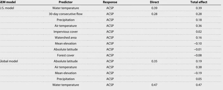
Table 2. Direct and total effects of each driver on ACSP in the U.S. and global models. Total effects are calculated as the sum of the direct and indirect effects of the predictor on the response variable.

SEM model Predictor Response Direct Total effect

U.S. model Water temperature ACSP 0.39 0.39

30-day consecutive flow ACSP 0.28 0.28

Precipitation ACSP 0.18

Air temperature ACSP 0.36

Impervious cover ACSP 0.02

Watershed area ACSP 0.16

Mean elevation ACSP −0.10

Absolute latitude ACSP −0.01

Forest cover ACSP −0.08

Global model Absolute latitude ACSP 0.35 0.19

Air temperature ACSP 0.38

Mean elevation ACSP −0.19

Precipitation ACSP 0.05

Water temperature ACSP 0.47 0.47

(7)

Hydrologic modeling

Hydrologic indices were independently predicted for each U.S. site, using time series of daily discharge records from the U.S. Geological Survey (USGS) Water Services portal (https://waterservices.usgs.

gov), and appended to the ACSP dataset. We began by selecting a national sample of flow gauges from the USGS Geospatial Attributes of Gages for Evaluating Streamflow database [GAGES II; Falcone et al.

(82)] that featured (nearly) continuous discharge records from 1970 through the present day; this duration allowed robust characteriza- tion of contemporary flow dynamics while maximizing the number and spatial distribution of gauges used to develop hydrologic models.

We then removed gauges with upstream impoundments of >50 Ml (megaliters) km⁻² (impoundment volume scaled by watershed area), as these sites may be more strongly influenced by dam release oper- ations than natural precipitation and land-use factors (83). This screening process resulted in a sample of 2568 gauges.

Random forest models were then developed for a set of hydrologic indices, incorporating four of five hydrologic components:

flow magnitude, frequency, duration, and rate of change (84). We began with models of 12 hydrologic indices that are broadly repre- sentative of perennial streams in a variety of conditions (85, 86). Flow magnitude was characterized by variability, skewness, two measures of spread, and median annual maximum flow. Flow frequency was characterized by low flow pulse percentage, frequency of low flow events, and two measures of high flood pulse percentage. Flow duration was characterized by the 30-day minimum and maximum daily discharge. Rate of change was characterized by hydrologic flashiness (87). Following Carlisle et al. (88), random forest models (500 iterations per model) were built for each flow index using the randomForest library in R (89). Each random forest model was parameterized with a suite of predictor variables representing precipitation, underlying geology, and land use, but excluding predictor variables that were subsequently used in SEMs of secondary production (forest cover, watershed size, and impervious surface in the upstream watershed). Random forest model fit differed among hydrologic indices, and we focused on those models that explained ≥45% of the variance in their respective indices. These included flashiness, high flow pulse percentage (i.e., number of daily values within a time series) exceeding the daily median by ×7 (HighFlowPulse7) and ×3 margins (HighFlowPulse3), minimum consecutive 30-day flow, low flow pulse percentage, and variation in daily flow. The final six random forest models were then used to predict flow indices at each of the stream sites included in the U.S.ACSP database.

Data analyses

A subset of 13 covariates (see Table 1), each representative of a hypothesized ACSP driver as shown in Fig. 1, was first selected for univariate regression analyses of U.S. streams. Associations between these covariates and ACSP were then independently tested with regression models of the general form ACSP = b × C + Y, where C is the covariate of interest, b is a coefficient (i.e., regression model slope) relating C to ACSP, and Y is an intercept term. Natural log transformations were used to improve normality for covariates with skewed distributions. In cases where C was a categorical variable (e.g., stream order), b was calculated for each categorical level in com- parison to a baseline level. For example, the stream order baseline was first-order (i.e., the smallest) streams. Thus, b for second-order streams was the difference between first- and second-order streams.

Because measurement units differed among covariates, standardized regression model parameter estimates were calculated [ (90)] to facilitate direct comparisons among covariates. Coefficients of de- termination (r²) were also calculated for each regression model to estimate the variation in ACSP explained by the respective covariate.

Next, SEM was used to confront the ACSP metamodel (Fig. 1) with the empirical ACSP and covariate data (table S1). This allowed us to (i) assess the complete graphical network of hypothesized interactions and relationships, with the directions of links (i.e., paths) in the SEM diagram indicating causal influences, and (ii) test the overall fit of the network (31, 91). Separate models were fit to the U.S. and global databases, with the former used to test the complete network of interrelationships among covariates shown in Fig. 1 and the latter testing for generality of the U.S. results at the global scale.

At each of the two scales, an iterative process of testing and linking covariates, consistent with the hypotheses outlined in the metamodel, was used to produce a final SEM of ACSP. Three indices of model fit were used with conventional significance thresholds—the ² P value (² P > 0.05), the standardized root mean squared residual (SRMR ≤ 0.08), and the comparative fit index (CFI ≥ 0.95)—to assess the overall fit of each SEM (92). All SEM procedures were conducted with the lavaan library in R (93). Code to build the final U.S. and global models is provided in data file S4.

SUPPLEMENTARY MATERIALS

Supplementary material for this article is available at http://advances.sciencemag.org/cgi/

content/full/5/4/eaav2348/DC1 Supplementary Materials and Methods

Fig. S1. Maps of study sites included in the ACSP database.

Table S1. Data dictionary for variables included in the secondary production database for U.S.

streams.

Data file S1. Citation records for all studies included in the ACSP database.

Data file S2. Complete secondary production and covariate data for all U.S. streams.

Data file S3. Secondary production and covariate data for the global streams database.

Data file S4. R code to build the U.S and global SEM models.

References (98–102)

REFERENCES AND NOTES

1. A. D. Huryn, J. B. Wallace, Life history and production of stream insects. Annu. Rev.

Entomol. 45, 83–110 (2000).

2. R. O. Hall Jr., J. B. Wallace, S. L. Eggert, Organic matter flow in stream food webs with reduced detrital resource base. Ecology 81, 3445–3463 (2000).

3. A. C. Benke, J. B. Wallace, High secondary production in a Coastal Plain river is dominated by snag invertebrates and fuelled mainly by amorphous detritus. Freshw. Biol. 60, 236–255 (2015).

4. G. Woodward, D. C. Speirs, A. G. Hildrew, Quantification and resolution of a complex, size-structured food web. Adv. Ecol. Res. 36, 85–135 (2005).

5. W. F. Cross, C. V. Baxter, E. J. Rosi-Marshall, R. O. Hall Jr., T. A. Kennedy, K. C. Donner, H. A. Wellard Kelly, S. E. Z. Seegert, K. E. Behn, M. D. Yard, Food-web dynamics in a large river discontinuum. Ecol. Monogr. 83, 311–337 (2013).

6. D. P. Whiting, M. R. Whiles, M. L. Stone, Patterns of macroinvertebrate production, trophic structure, and energy flow along a tallgrass prairie stream continuum. Limnol. Oceanogr.

56, 887–898 (2011).

7. M. R. Whiles, J. B. Wallace, Macroinvertebrate production in a headwater stream during recovery from anthropogenic disturbance and hydrologic extremes. Can. J. Fish. Aq. Sci.

52, 2402–2422 (1995).

8. D. M. Carlisle, W. H. Clements, Growth and secondary production of aquatic insects along a gradient of Zn contamination in Rocky Mountain streams. J. N. Am. Benthol. Soc. 22, 582–597 (2003).

9. N. S. Ismail, C. E. Müller, R. R. Morgan, R. G. Luthy, Uptake of contaminants of emerging concern by the bivalves Anodonta californiensis and Corbicula fluminea. Environ. Sci.

Technol. 48, 9211–9219 (2014).

10. National Research Council, Ecosystem services of bivalves: Implications for restoration, in Ecosystem Concepts for Sustainable Bivalve Mariculture (National Academies Press, 2010), pp. 123–132.

(8)

11. E. Mortensen, J. L. Simonsen, Production estimates of the benthic invertebrate community in a small Danish stream. Hydrobiologia 102, 155–162 (1983).

12. M. A. Wilzbach, K. W. Cummins, J. D. Hall, Influence of habitat manipulations on interactions between cutthroat trout and invertebrate drift. Ecology 67, 898–911 (1986).

13. A. D. Huryn, Growth and voltinism of lotic midge larvae: Patterns across an Appalachian Mountain basin. Limnol. Oceanogr. 35, 339–351 (1990).

14. A. D. Huryn, A. C. Benke, G. M. Ward, Direct and indirect effects of geology on the distribution, biomass, and production of the freshwater snail Elimia. J. N. Am. Benthol. Soc.

14, 519–534 (1995).

15. A. Morin, P. Dumont, A simple model to estimate growth rate of lotic insect larvae and its value for estimating population and community production. J. N. Am. Benthol. Soc. 13, 357–367 (1994).

16. D. Nelson, J. P. Benstead, A. D. Huryn, W. F. Cross, J. M. Hood, P. W. Johnson, J. R. Junker, G. M. Gíslason, J. S. Ólafsson, Shifts in community size structure drive temperature invariance of secondary production in a stream-warming experiment. Ecology 98, 1797–1806 (2017).

17. A. C. Benke, A. D. Huryn, Secondary production and quantitative food webs, in Stream Ecology. Volume 2: Ecosystem Function (Elsevier, ed. 3, 2017), pp. 235–254.

18. A. P. Covich, M. A. Palmer, T. A. Crowl, The role of benthic invertebrate species in freshwater ecosystems: Zoobenthic species influence energy flows and nutrient cycling.

Bioscience 49, 119–127 (1999).

19. D. Nelson, J. P. Benstead, A. D. Huryn, W. F. Cross, J. M. Hood, P. W. Johnson, J. R. Junker, G. M. Gíslason, J. S. Ólafsson, Experimental whole-stream warming alters community size structure. Glob. Chang. Biol. 23, 2618–2628 (2017).

20. A. C. Benke, M. R. Whiles, Life table vs secondary production analyses—Relationships and usage in ecology. J. N. Am. Benthol. Soc. 30, 1024–1032 (2011).

21. A. C. Benke, Secondary production as part of bioenergetic theory—Contributions from freshwater benthic science. River Res. Appl. 26, 36–44 (2010).

22. C. Segura, P. Caldwell, G. Sun, S. McNulty, Y. Zhang, A model to predict stream water temperature across the conterminous USA. Hydrol. Process. 29, 2178–2195 (2015).

23. P. J. Mulholland, C. S. Fellows, J. L. Tank, N. B. Grimm, J. R. Webster, S. K. Hamilton, E. Martí, L. Ashkenas, W. B. Bowden, W. K. Dodds, W. H. Mcdowell, M. J. Paul, B. J. Peterson, Inter-biome comparison of factors controlling stream metabolism. Freshw. Biol. 46, 1503–1517 (2001).

24. B. O. L. Demars, J. R. Manson, J. S. Ólafsson, G. M. Gíslason, R. Gudmundsdóttir, G. Woodward, J. Reiss, D. E. Pichler, J. J. Rasmussen, N. Friberg, Temperature and the metabolic balance of streams. Freshw. Biol. 56, 1106–1121 (2011).

25. E. R. Hannesdóttir, G. M. Gíslason, J. S. Ólafsson, Ó. P. Ólafsson, E. J. O’Gorman, Increased stream productivity with warming supports higher trophic levels. Adv. Ecol. Res. 48, 285–342 (2013).

26. N. B. Grimm, S. G. Fisher, Stability of periphyton and macroinvertebrates to disturbance by flash floods in a desert stream. J. N. Am. Benthol. Soc. 8, 293–307 (1989).

27. R. G. Death, The effect of habitat stability on benthic invertebrate communities:

The utility of species abundance distributions. Hydrobiologia 317, 97–107 (1996).

28. I. G. Jowett, Hydraulic constraints on habitat suitability for benthic invertebrates in gravel-bed rivers. River Res. Appl. 19, 495–507 (2003).

29. P. D. Markos, M. D. Kaller, W. E. Kelso, Channel stability and the structure of coastal stream aquatic insect assemblages. Fundam. Appl. Limnol. 188, 187–199 (2016).

30. J. B. Grace, D. R. Schoolmaster Jr., G. R. Guntenspergen, A. M. Little, B. R. Mitchell, K. M. Miller, E. W. Schweiger, Guidelines for a graph-theoretic implementation of structural equation modeling. Ecosphere 3, 1–44 (2012).

31. J. B. Grace, Structural Equation Modeling and Natural Systems (Cambridge Univ. Press, Cambridge, 2006).

32. A. C. Benke, Concepts and patterns of invertebrate production in running waters.

Verh. Int. Ver. Theor. Angew. Limnol. 25, 15–38 (1993).

33. L. R. Harrison, C. J. Legleiter, M. A. Wydzga, T. Dunne, Channel dynamics and habitat development in a meandering, gravel bed river. Water Resour. Res. 47, W04513 (2011).

34. K. M. Potter, F. W. Cubbage, R. H. Schaberg, Multiple-scale landscape predictors of benthic macroinvertebrate community structure in North Carolina. Landscape Urban Plann. 71, 77–90 (2005).

35. J. C. Rutherford, S. Blackett, C. Blackett, L. Saito, R. J. Davies-Colley, Predicting the effects of shade on water temperature in small streams. N. Z. J. Mar. Freshwat. Res. 31, 707–721 (1997).

36. D. Caissie, The thermal regime of rivers: A review. Freshw. Biol. 51, 1389–1406 (2006).

37. J. C. Morrill, R. C. Bales, M. H. Conklin, Estimating stream temperature from air temperature: Implications for future water quality. J. Environ. Eng. 131, 139–146 (2005).

38. L. L. Larry, L. L. Shane, Riparian shade and stream temperature: A perspective.

Rangelands 18, 149–152 (1996).

39. G. C. Poole, C. H. Berman, An ecological perspective on in-stream temperature: Natural heat dynamics and mechanisms of human-caused thermal degradation. Environ. Manag.

27, 787–802 (2001).

40. M. A. Rahman, A. Moser, T. Rötzer, S. Pauleit, Within canopy temperature differences and cooling ability of Tilia cordata trees grown in urban conditions. Build. Environ. 114, 118–128 (2017).

41. J. H. Brown, J. F. Gillooly, A. P. Allen, V. M. Savage, G. B. West, Toward a metabolic theory of ecology. Ecology 85, 1771–1789 (2004).

42. C. B. Field, M. J. Behrenfeld, J. T. Randerson, P. Falkowski, Primary production of the biosphere: Integrating terrestrial and oceanic components. Science 281, 237–240 (1998).

43. J. S. Richardson, Seasonal food limitation of detritivores in a montane stream:

An experimental test. Ecology 72, 873–887 (1991).

44. B. J. Peterson, L. Deegan, J. Helfrich, J. E. Hobbie, M. Hullar, B. Moller, T. E. Ford, A. Hershey, A. Hiltner, G. Kipphut, M. A. Lock, D. M. Fiebig, V. McKinley, M. C. Miller, J. R. Vestal, R. Ventullo, G. Volk, Biological responses of a tundra river to fertilization.

Ecology 74, 653–672 (1993).

45. J. B. Wallace, S. L. Eggert, J. L. Meyer, J. R. Webster, Effects of resource limitation on a detrital-based ecosystem. Ecol. Monogr. 69, 409–442 (1999).

46. T. M. Iversen, Ingestion and growth in Sericostoma personatum (Trichoptera) in relation to the nitrogen content of ingested leaves. Oikos 25, 278–282 (1974).

47. G. M. Ward, K. W. Cummins, Effects of food quality on growth of a stream detritivore, Paratendipes Albimanus (Meigen) (Diptera: Chironomidae). Ecology 60, 57–64 (1979).

48. C. L. Fuller, M. A. Evans-White, S. A. Entrekin, Growth and stoichiometry of a common aquatic detritivore respond to changes in resource stoichiometry. Oecologia 177, 837–848 (2015).

49. W. F. Cross, J. B. Wallace, A. D. Rosemond, S. L. Eggert, Whole-system nutrient enrichment increases secondary production in a detritus-based ecosystem. Ecology 87, 1556–1565 (2006).

50. J. B. Wallace, S. L. Eggert, J. L. Meyer, J. R. Webster, Multiple trophic levels of a forest stream linked to terrestrial litter inputs. Science 277, 102–104 (1997).

51. W. K. Dodds, Eutrophication and trophic state in rivers and streams.

Limnol. Oceanogr. 51, 671–680 (2006).

52. F. Woodward, Climate and Plant Distribution (Cambridge Univ. Press, 1987).

53. A. Hoffman, P. Parsons, Extreme Environmental Change and Evolution (Cambridge Univ.

Press, 1997).

54. P. B. Reich, J. Oleksyn, Global patterns of plant leaf N and P in relation to temperature and latitude. Proc. Natl. Acad. Sci. U.S.A. 101, 11001–11006 (2004).

55. W. K. Dodds, K. Gido, M. R. Whiles, M. D. Daniels, B. P. Grudzinski, The stream biome gradient concept: Factors controlling lotic systems across broad biogeographic scales.

Freshw. Sci. 34, 1–19 (2015).

56. B. Bond-Lamberty, S. D. Peckham, D. E. Ahl, S. T. Gower, Fire as the dominant driver of central Canadian boreal forest carbon balance. Nature 450, 89–92 (2007).

57. M. Zhao, S. W. Running, Drought-induced reduction in global terrestrial net primary production from 2000 through 2009. Science 329, 940–943 (2010).

58. M. Piniewski, C. Prudhomme, M. C. Acreman, L. Tylec, P. Oglęcki, T. Okruszko, Responses of fish and invertebrates to floods and droughts in Europe. Ecohydrology 10, e1793 (2017).

59. J. Jackson, S. G. Fisher, Secondary production, emergence, and export of aquatic insects of a Sonoran Desert stream. Ecology 67, 629–638 (1986).

60. J. E. Gladden, L. A. Smock, Macroinvertebrate distribution and production on the floodplains of two lowland headwater streams. Freshw. Biol. 24, 533–545 (1990).

61. R. O. Hall Jr., M. F. Dybdahl, M. C. VanderLoop, Extremely high secondary production of introduced snails in rivers. Ecol. Appl. 16, 1121–1131 (2006).

62. M. A. Chadwick, A. D. Huryn, Role of habitat in determining macroinvertebrate production in an intermittent-stream system. Freshw. Biol. 52, 240–251 (2007).

63. M. E. Ledger, F. K. Edwards, L. E. Brown, A. M. Milner, G. Woodward, Impact of simulated drought on ecosystem biomass production: An experimental test in stream mesocosms.

Glob. Chang. Biol. 17, 2288–2297 (2011).

64. N. Majdi, B. Mialet, S. Boyer, M. Tackx, J. Leflaive, S. Boulêtreau, L. Ten-Hage, F. Julien, R. Fernandez, E. Buffan-Dubau, The relationship between epilithic biofilm stability and its associated meiofauna under two patterns of flood disturbance.

Freshw. Sci. 31, 38–50 (2012).

65. S. G. Fisher, L. J. Gray, N. B. Grimm, D. E. Busch, Temporal succession in a desert stream ecosystem following flash flooding. Ecol. Monogr. 52, 93–110 (1982).

66. G. G. Mittelbach, C. F. Steiner, S. M. Scheiner, K. L. Gross, H. L. Reynolds, R. B. Waide, M. R. Willig, S. I. Dodson, L. Gough, What is the observed relationship between species richness and productivity? Ecology 82, 2381–2396 (2001).

67. B. J. Cardinale, D. S. Srivastava, J. Emmett Duffy, J. P. Wright, A. L. Downing, M. Sankaran, C. Jouseau, Effects of biodiversity on the functioning of trophic groups and ecosystems.

Nature 443, 989–992 (2006).

68. B. Statzner, V. H. Resh, Multiple-site and-year analyses of stream insect emergence: A test of ecological theory. Oecologia 96, 65–79 (1993).

69. M. R. Whiles, B. S. Goldowitz, Hydrologic influences on insect emergence production from Central Platte River WETLANDS. Ecol. Appl. 11, 1829–1842 (2001).

70. M. R. Vinson, C. P. Hawkins, Broad-scale geographical patterns in local stream insect genera richness. Ecography 26, 751–767 (2003).

(9)

71. L. A. Bêche, B. Statzner, Richness gradients of stream invertebrates across the USA:

Taxonomy- and trait-based approaches. Biodivers. Conserv. 18, 3909–3930 (2009).

72. J. C. Finlay, Stream size and human influences on ecosystem production in river networks. Ecosphere 2, 1–21 (2011).

73. Intergovernmental Panel on Climate Change, "AR5 synthesis report: Climate change 2014" (Technical Report, 2014).

74. R. Allen, B. Soden, Atmospheric warming and the amplification of precipitation extremes.

Science 321, 1481–1484 (2008).

75. R. Seager, M. Ting, C. Li, N. Naik, B. Cook, J. Nakamura, H. Liu, Projections of declining surface-water availability for the southwestern United States. Nat. Clim. Chang. 3, 482–486 (2013).

76. R. Seager, M. Ting, I. Held, Y. Kushnir, J. Lu, G. Vecchi, H. P. Huang, N. Harnik, A. Leetmaa, N. C. Lau, C. Li, J. Velez, N. Naik, Model projections of an imminent transition to a more arid climate in southwestern North America. Science 316, 1181–1184 (2007).

77. A. Dai, Increasing drought under global warming in observations and models.

Nat. Clim. Chang. 3, 52–58 (2013).

78. N. L. Poff, J. D. Olden, N. K. M. Vieira, D. S. Finn, M. P. Simmons, B. C. Kondratieff, Functional trait niches of North American lotic insects: Traits-based ecological applications in light of phylogenetic relationships. J. N. Am. Benthol. Soc. 25, 730–755 (2006).

79. J. C. White, D. M. Hannah, A. House, S. J. V. Beatson, A. Martin, P. J. Wood, Macroinvertebrate responses to flow and stream temperature variability across regulated and non-regulated rivers. Ecohydrology 10, e1773 (2017).

80. D. G. Jenkins, Estimating ecological production from biomass. Ecosphere 6, 1–31 (2015).

81. T. F. Waters, Secondary production in inland waters. Adv. Ecol. Res. 10, 91–164 (1977).

82. J. A. Falcone, D. M. Carlisle, D. M. Wolock, M. R. Meador, GAGES: A stream gage database for evaluating natural and altered flow conditions in the conterminous United States.

Ecology 91, 621 (2010).

83. L. L. Yuan, Using correlation of daily flows to identify index gauges for ungauged streams. Water Resour. Res. 49, 604–613 (2013).

84. N. L. Poff, J. D. Allan, M. B. Bain, J. R. Karr, K. L. Prestegaard, B. D. Richter, R. E. Sparks, J. C. Stromberg, The natural flow regime. Bioscience 47, 769–784 (1997).

85. J. D. Olden, N. L. Poff, Redundancy and the choice of hydrologic indices for characterizing streamflow regimes. River Res. Appl. 19, 101–121 (2003).

86. C. J. Patrick, L. L. Yuan, Modeled hydrologic metrics show links between hydrology and the functional composition of stream assemblages. Ecol. Appl. 27, 1605–1617 (2017).

87. D. B. Baker, R. P. Richards, T. T. Loftus, J. W. Kramer, A new flashiness index: Characteristics and applications to midwestern rivers and streams. J. Am. Water Resour. Assoc. 40, 503–522 (2004).

88. D. M. Carlisle, D. M. Wolock, M. R. Meador, Alteration of streamflow magnitudes and potential ecological consequences: A multiregional assessment. Front. Ecol. Environ. 9, 264–270 (2010).

89. D. R. Cutler, T. C. Edwards Jr., K. H. Beard, A. Cutler, K. T. Hess, J. Gibson, J. J. Lawler, Random forests for classification in ecology. Ecology 88, 2783–2792 (2007).

90. J. R. Hair, R. C. Anderson, R. Tatham, W. Black, Multivariate Data Analysis (Prentice Hall, ed. 5, 1998).

91. B. Shipley, Cause and Correlation in Biology: A User’s Guide to Path Analysis, Structural Equations and Causal Inference (Cambridge Univ. Press, 2002).

92. L. Hu, P. M. Bentler, Cutoff criteria for fit indexes in covariance structure analysis:

Conventional criteria versus new alternatives. Struct. Equ. Modeling 6, 1–55 (1999).

93. Y. Rosseel, lavaan: An R Package for structural equation modeling. J. Stat. Softw. 48 (2012).

94. N. J. Hetrick, M. A. Brusven, W. R. Meehan, T. C. Bjornn, Changes in solar input, water temperature, periphyton accumulation, and allochthonous input and storage after

canopy removal along two small salmon streams in southeast Alaska. Trans. Am. Fish. Soc.

127, 859–875 (1998).

95. O. Mohseni, T. R. Erickson, H. G. Stefan, Upper bounds for stream temperatures in the contiguous United States. J. Environ. Eng. 128, 4–11 (2002).

96. R. L. Vannote, G. W. Minshall, K. W. Cummins, J. R. Sedell, C. E. Cushing, The river continuum concept. Can. J. Fish. Aquat. Sci. 37, 130–137 (1980).

97. M. Diana, J. D. Allan, D. Infante, The influence of physical habitat and land use on stream fish assemblages in southeastern Michigan. Am. Fish. Soc. Symp. 48, 359–374 (2006).

98. L. McKay, T. Bondelid, T. Dewald, A. Rea, C. Johnston, R. Moore, NHDPlus Version 2: User Guide (Data Model Version 2.1) (Horizon Systems, 2015).

99. R. A. Hill, M. H. Weber, S. G. Leibowitz, A. R. Olsen, D. J. Thornbrugh, The Stream- Catchment (StreamCat) dataset: A database of watershed metrics for the conterminous United States. J. Am. Water Resour. Assoc. 52, 120–128 (2016).

100. L. Breiman, Random forests. Mach. Learn. 45, 5–32 (2001).

101. D. M. Carlisle, J. Falcone, D. M. Wolock, M. R. Meador, R. H. Norris, Predicting the natural flow regime: Models for assessing hydrological alteration in streams. River Res. Appl. 26, 118–136 (2010).

102. C. K. Wentworth, A scale of grade and class terms for clastic sediments. J. Geol. 30, 377–392 (1922).

Acknowledgments

Funding: We thank the U.S. NSF (grant no. DEB-1354867) for funding the Stream Resiliency Research Coordination Network (RCN) and the National Center for Ecological Analysis and Synthesis (NCEAS) for hosting the Structural Equation and Mechanistic Modeling Working Group, where many of these ideas were developed. C.J.P. received additional support from the National Academy of Science, Engineering, and Medicine (GRP-ECRF). D.J.M. received additional support through the NSF (DEB-1553111). G.W. was supported by the UK Natural Environment Research Council Large Grant (NE/M020843/1). W.F.C. received additional support through the NSF (DEB-0949774). Graphic icons used in Figs. 1 and 2 were downloaded from Freepik (www.freepik.com) and the Integration and Application Network, University of Maryland Center for Environmental Science (ian.umces.edu/imagelibrary/).

Author contributions: All authors contributed to the development of the dataset used in these analyses and writing and editing of the manuscript and supplementary documents.

C.J.P. was responsible for the hydrologic modeling. D.J.M. was responsible for the geospatial analyses. C.J.P., D.J.M., and J.H.L. were responsible for the statistical analyses. Competing interests: The authors declare that they have no competing interests. Data and materials availability: All data needed to evaluate the conclusions in the paper are present in the paper and/or the Supplementary Materials. Additional data related to this paper may be requested from the authors.

Submitted 28 August 2018 Accepted 27 February 2019 Published 17 April 2019 10.1126/sciadv.aav2348

Citation: C. J. Patrick, D. J. McGarvey, J. H. Larson, W. F. Cross, D. C. Allen, A. C. Benke, T. Brey, A. D. Huryn, J. Jones, C. A. Murphy, C. Ruffing, P. Saffarinia, M. R. Whiles, J. B. Wallace, G. Woodward, Precipitation and temperature drive continental-scale patterns in stream invertebrate production.

Sci. Adv. 5, eaav2348 (2019).

(10)

Murphy, C. Ruffing, P. Saffarinia, M. R. Whiles, J. B. Wallace and G. Woodward

DOI: 10.1126/sciadv.aav2348 (4), eaav2348.

5 Sci Adv

ARTICLE TOOLS http://advances.sciencemag.org/content/5/4/eaav2348

MATERIALS

SUPPLEMENTARY http://advances.sciencemag.org/content/suppl/2019/04/12/5.4.eaav2348.DC1

REFERENCES

http://advances.sciencemag.org/content/5/4/eaav2348#BIBL This article cites 92 articles, 6 of which you can access for free

PERMISSIONS http://www.sciencemag.org/help/reprints-and-permissions

Terms of Service Use of this article is subject to the

registered trademark of AAAS.

is a Science Advances Association for the Advancement of Science. No claim to original U.S. Government Works. The title

York Avenue NW, Washington, DC 20005. 2017 © The Authors, some rights reserved; exclusive licensee American (ISSN 2375-2548) is published by the American Association for the Advancement of Science, 1200 New Science Advances