Master Thesis Development of a statistical daily precipitation model and its application to precipitation records

Master Thesis

Development of a statistical daily precipitation model and its

application to precipitation records

Recombination and Speciation on Fitness Landscapes

Alexander Klug and Joachim Krug

Institute for Theoretical Physics, University of Cologne

Fitness landscape

• Genotypes are defined by sequences:

σ = (σ ₁ , σ ₂ , ..., σ _L )

• Entries are denoted as locus points and con- tain one of a variety of alleles, e.g.

– Nucleotides σ _i = { G, A, C, T }

– Entire genes σ _i = { gene ₁ , gene ₂ , ... }

• Here a binary system is used in the sense that only two different alleles are assumed:

σ _i = { 0, 1 }

• A metric is introduced by the hamming dis- tance d, which counts the loci in which two genotypes differ: d(σ, κ) = 1 → genotypes σ, κ adjacent

• For a binary system this creates a hypercube of dimension L, consisting of 2 ^L genotypes

• Finally the fitness landscape is a mapping from genotypes to their fitness F (σ ) = w _σ , which is a measure of their reproductive suc- cess

Evolutionary model

• Discrete deterministic Wright-Fisher dynam- ics in the limit of inifinte populations is used

• Since the number of individuals N is taken to infinity the frequency f _σ (t) of each genotype σ at time t in the population is of interest

• Average fitness of the population:

¯

w(t) = X

σ

w _σ f _σ (t)

• Evolution in the presence of selection and mu- tation:

f ˜ _σ (t) = X

κ

U _σκ w _κ

¯

w(t) f _κ (t)

• Mutations occur at each locus with the same probability µ . Multiple mutations are possible but less likely:

U _σκ = (1 − µ) ^{L − d(σ,κ)} µ ^d(σ,κ)

• After selection and mutation, recombination takes place:

f _σ (t + 1) = X

τ κ

R _{σ | τ κ} f ˜ _τ (t) ˜ f _κ (t)

• R _{σ | τ κ} describes the probability that two geno- types τ and κ recombine to third genotype σ which creates a tensor of rank three.

• For a uniform crossover with two loci and a tunable recombination rate r:

(σ ₁ σ ₂ )

(κ ₁ κ ₂ ) →

 

 

 

 

 



(σ ₁ κ ₂ ) (κ ₁ σ ₂ )

)

with prop. r 2 (σ ₁ σ ₂ )

(κ ₁ κ ₂ )

)

with prop. 1 − r 2

Two-Locus landscape and reciprocal sign epistasis

• Reciprocal sign epistasis: The sign of a muta- tion effect at locus i depends on j and vice versa

• Necessary condition for the appearance of dif- ferent local fitness peaks, which in turn can hin- der the population to reach the global optimum

• This so-called local peak trapping is even stronger for recombining populations, in the sense that the escape time increases

• The escape time diverge at a critical recombi- nation rate r _c

• In the limit of infinite populations distinct sta- tionary states emerge

0.0 0.2 0.4 0.6 0.8 1.0

0.0 0.2 0.4 0.6 0.8

0.002 0.008

0.1 0.3 0.5 0.7

Empirical landscape

0 1 2 3 4 5 6 7 8

Hamming distance

0.0 0.2 0.4 0.6 0.8 1.0

Fitness value

Empirical model: Aspergillus niger

0 1 2 3 4 5 6 7

Hamming distance

0.7 0.8 0.9 1.0

Fitness value

26

6

7 6 3

3 20

282 16

35 20

18

All stationary states overlapped with =0.001 and r=1.0

Local maxima Recombination center

Recombination center

χ = max( X

τ κ

R _{σ | τ κ} w _τ w _κ , ∀ σ )

References

• P. G. Higgs, Genetica 102/103: 91– 101 (1998)

• S. Park, J. Krug, J. Math. Biol. 62:763- 788 (2011)

• J. Franke, A. Klözer, J.A.G.M. de Visser, J. Krug, PLoS Comput Biol 7(8): e1002134 (2011)

• S. Gavrilets, Trends Ecol. Evol. 12:307- 12 (1997)

• T. Paixao, K. E. Bassler, R. B. R. Azevedo, bioRxiv 008268

• E. van Nimwegen, J. P. Crutchfield, M. Huynen, PNAS 96:9716- 9720 (1999)

Percolation landscape

Percolation landscape

Lethal genotypes Viable genotypes Recombination center

244

1

2 24

9

1 7 1

1 1 1

1 1

3 4

4 2

2 1

1 6

1

All stationary states overlapped with =0.01 and r=1.0

Local maxima Recombination center

Mutational robustness

DMI’s

submitted by

Philipp von Bomhard to achieve the academic degree

Master of Science

1

Supervisor: Prof. Dr. Yaping Shao 2

Supervisor: Prof. Dr. Joachim Krug

Köln, 08.09.2017

Abstract

In recent years, numerous record-breaking precipitation events have caused several

deaths and high economic losses. However, current precipitation models do not ad-

equately capture exceptionally high precipitation events. To address this problem,

a new statistical daily precipitation model including several new aspects was de-

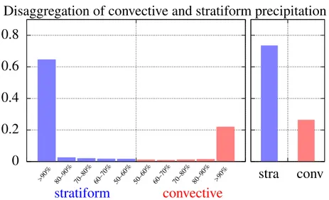
veloped. The model distinguishes between stratiform and convective precipitation,

whereby the disaggregation of these two types of precipitation is based on SYNOP

reports of 300 German weather stations. By combining a Weibull distribution with

power law, a new probability distribution was derived and later implemented in

the amount process. This four-parameter distribution improves the modelling of

extreme precipitation amounts enormously and still delivers good results for small

amounts. To take account of variability, a conned random walk was additionally

implemented in the occurrence process of the model. The model was developed in

a manner that allows universal use. By incorporating the elevation of a station and

the time of the year as input parameters, the model was made applicable at any time

and for any location in Germany. In a second step the model was applied to investi-

gate daily precipitation records. For that, linear changes were implemented into the

model. As result, a previously found decrease of records in the summer season can

be explained by changes in the stratiform precipitation distribution. However, the

decrease of precipitation records in the summer season is too low to rule out random

processes as cause of this decrease. In contrast, the increase in the mean number

of precipitation records in winter season cannot be reproduced with the developed

model. A possible explanation for that is the neglect of spatial correlations in the

amount process. An appropriate method for taking spatial correlations into account,

could be a Copula approach.

Table of Contents

1. Introduction 5

1.1. Precipitation models . . . . 8

1.1.1. The occurrence process . . . . 8

1.1.2. The amount process . . . 11

1.2. Records . . . 14

1.3. Aim . . . 18

2. Data and data processing 19 2.1. Dataset DWD

. . . 19

2.2. Dataset DWD

. . . 21

2.3. SYNOP-Dataset . . . 21

2.4. Disaggregating convective and stratiform precipitation . . . 23

3. Development of a precipitation model 27 3.1. Development of the occurrence process . . . 28

3.2. Development of the amount process . . . 33

3.2.1. Development of a distribution for precipitation . . . 33

3.2.2. Time and altitude dependence . . . 40

3.3. Taking account of variability in the occurrence process . . . 42

3.4. Model results vs. observation . . . 44

3.4.1. Precipitation occurrence . . . 44

3.4.2. Precipitation amounts . . . 46

4. Application to precipitation records 48 4.1. Observed changes in the past . . . 48

4.1.1. Observed changes in the occurrence process . . . 49

4.1.2. Observed changes in the amount process . . . 50

4.2. Implementation of a drift in the precipitation model . . . 52

4.3. Modelled precipitation records . . . 55

5. Conclusion and Outlook 58

3

Appendix 63

Bibliography 68

Acknowledgements 75

1. Introduction

Precipitation is essential for life. It provides water for the continents, an important prerequisite for life on earth. When there are reduced amounts or even a lack of rain over a longer period of time, there are widespread consequences: increased risk of res, shortage in water- and power supply as well as crop shortfall and resulting increase in food prices. A well-known example is the heatwave in Central Europe in 2003: a long lasting dry spell in combination with extremely high temperatures lead to 70,000 fatalities and a nancial loss of US$ 13.8bn [Robine et al. (2008); Munich RE (2017)]. Another example was the dry spell in November 2011 in which a mean precipitation of 3mm lead to the driest month ever recorded in Germany since the beginning of comprehensive weather records in 1881 [Müller-Westermeier (2012)].

On the other hand, high amounts of precipitation over a long period of time also have negative consequences, especially for agriculture. Crops cannot be harvested and are often spoiled if it is too wet. The most fatal situations often occur when extremely high amounts of precipitation are limited to a very short period of time leading to ooding and high economic losses. The highest daily precipitation ever recorded in Germany was 312mm, measured in Zinnwald-Georgenfeld on August 12th 2002 [Rudolf and Rapp (2003)]. In the following weeks, the area around the river Elbe suered from devastating ooding. There was an economic damage of US$ 11.6bn [Munich RE (2017)] in Germany. In May 2013, there was another ex- treme ooding in south and eastern Germany: Even if the highest daily precipitation was far below previously reported records in 2002, the month May was the second wettest since 1881. Several local records were recorded in May and June [DWD (2013)] and the overall losses were estimated to US$ 10.4bn [Munich RE (2017)].

In the summer months of previous years heavy precipitation was mainly observed very locally in Germany. This summer ocial 197mm of rain were recorded within several hours in Berlin by the German Weather Service while daily rain totals of a private weather station even exceeded 260mm [Gebauer et al. (2017)]. Even more rain in a shorter period of time was recorded in Münster in July 2014: Within 7

5

Table 1.1.: List of the eight costliest hydrological events from 19802016, sorted by the convective percentage of the total rainfall amount in the given periods. The convective percentages were calculated by using SYNOP reports to disaggregate types of precipitation. Data source: Munich RE (2017) & SYNOP reports (see sec. 2).

.

Period Event Overall losses Fatalities Convective rain

28.07. 29.07.2014 Flash flood US$ 600m 2 27.05. 30.05.2016 Flash flood US$ 830m 4 31.05. 01.06.2016 Flash flood US$ 2,000m 7 16.07. 04.08.1997 Flood US$ 370m

25.05. 15.06.2013 Flood US$ 10,400m 8

06.08. 09.08.2010 Flood US$ 1,100m 4

04.08. 13.08.2002 Flood US$ 11,600m 21

17.12. 27.12.1993 Flood US$ 600m 5

Figure 1: Abbildungstext

hours 292mm and within just 2 hours 245mm of rain was measured [Becker et al.

(2014); Axer et al. (2015)]. The German Weather Service declared this 2-hour-value as a new German record [Becker et al. (2014)]. According to Munich RE (2017) this was the most expensive ash ood since 1980 with an overall damage of US$ 510m whereof US$ 230m was insured. However, in 2016 this record was even beaten twice:

In the small town of Braunsbach (Baden-Württemberg) damage of US$ 830m (US$

500m insured [Munich RE (2017)]) was caused by a ash ood on May 29th while only three days later a damage of US$ 2bn (US$ 830m insured [Munich RE (2017)]) in Simbach am Inn was caused by another ash ood. In Gundesheim, a town 50 km West of Braunsbach, a daily precipitation record of 122mm was recorded for the day of the ooding. The weather station close to Simbach am Inn did not record any values at the critical hours of the event but the total daily precipitation sum is expected to be similar of these in Gundelsheim [Piper et al. (2016)]. The discrep- ancy between the high overall damage and the relatively low measured precipitation amounts can be explained by the topographic position of Braunsbach and Simbach am Inn [Axer et al. (2017)].

The main cause of costly and destructive events can be identied by looking at the previously described examples: On the one hand heavy continuous rainfall can

6

Table 1.2.: Overview of typical characteristics of stratiform and convective precipitation.

stratiform convective

scale large-scale local

duration long short

intensity less intensive more intensive typical example large-scale frontal rain, thunderstorms,

drizzle showers

lead to supra-regional ooding (e.g. ooding in 2002 and 2013), on the other hand extreme local rainfalls can swamp the sewage water system leading to ash oods (e.g. ash ood events 2014 and 2016). In fact these two event types result from two major processes of precipitation generation: stratiform and convective precipitation (see Tab. 1.1). These two precipitation types dier in many aspects, such as the cloud type of which the precipitation falls out or the fall velocity of the rain drops in relation to the vertical air motion [Houze Jr (2014)]. Stratiform precipitation is characterized by long-lasting large-scale precipitation (e.g. drizzle) while convective precipitation is typically very local and more intensive but of short duration (e.g.

thunderstorms) (see Tab. 1.2 for a summary of the main dierences). Furthermore, it has a highly seasonal dependency with much more convective events occurring in summer compared to winter season.

The extreme precipitation events mentioned above are often associated with cli- mate change. According to the ClausiusClapeyron rate, the water holding capacity of the atmosphere increases by around 7% per degree warming. Since precipitation releases latent heat, the global total rainfall amount is expected to increase by just 1% 3% K

with warming [Solomon (2007); Stephens and Ellis (2008)]. However, according to the latest studies [Berg et al. (2013); Zhang et al. (2017)] the convective precipitation which is already very intense increases the most, even more than the Clausius-Clapeyron rate. This is probably due to local feedbacks related to the convective activity [Lenderink et al. (2017)]. The increase in the intensity of strong rainfall is expected to be associated with a decrease in light and moderate rains and/or a decline in the frequency of precipitation events [Trenberth et al. (2003)].

These ndings lead to the assumption that an increase in precipitation records is due to global warming. This is mainly true for the summer months in which more

7

convective precipitation events occur. The latest extreme precipitation events ob- served in Germany seem to validate this hypothesis. Surprisingly, an investigation of daily precipitation records in Germany [von Bomhard (2014)] led to an opposite result: in the summer months fewer records were observed than theoretically ex- pected in a stationary climate. However, in the winter months around 16% more records were observed than expected. The reason of the increased (winter) or de- creased (summer) precipitation records will be investigated in this work by using a newly developed statistical precipitation model (see also sec. 1.3).

The following subsections are intended to give a comprehensive overview of sta- tistical precipitation models (sec. 1.1) and record statistics (sec. 1.2).

1.1. Precipitation models

Generally stochastic precipitation models have two submodules: an occurrence pro- cess and an amount process. The occurrence process has to classify whether a certain day is a wet or a dry day. For dry days the precipitation amount is equal to zero but for a day to be classied a wet day the amount process has to determine a nonzero precipitation amount.

1.1.1. The occurrence process

Since the rst computer models were used for generating daily weather variables a lot of dierent possibilities for implementing the occurrence process were tested.

A recent work from Ng and Panu (2010) compares four dierent models based on the short-term temporal-dependency, dry- and wet-spell length and goodness-of- t. Using these three assessment criteria, a two state, second order Markov chain showed the best performance. In addition to the Markov chain the authors also investigated an alternating renewal process (ARP) and introduced the Dictionary approach (originally developed in the eld of genome pattern) and a probabilistic word matrix model referring to a list of words comprised of precipitation letters.

The ARP spell length model and the Markov chain model are well performing mod- els which are frequently used. These models will be discussed below in more detail.

For more details about additional approaches in the context of precipitation occur- rence processes see Ng and Panu (2010) and references therein.

8

Markov chain

In general, a Markov chain model is characterized by its order n a number of states m . In the context of rainfall, the Markov chain is usually implemented with two states (a dry day and a wet day). In addition to a wet state and a dry state some studies included a certain threshold for separating a state with little rainfall amounts from a state with higher rainfall amounts. For example, Stern and Coe (1984) dened a third trace state for days with precipitation amounts less than 2.5mm.

The order of the Markov chain can be imagined as the number of days the chain remembers (therefore also called memory depth). With an increasing order of the Markov chain process the number of required parameters increases exponentially.

For a two state, k -th order Markov chain 2

parameters are required. To deter- mine the optimum order of a Markov chain model for a given set of data, usually maximum likelihood based information criteria are used. These information criteria detect the goodness of t using a maximum likelihood but also include a penalty which increases with adding more parameters and therefore with a higher order of the process. Usually the Akaike Information Criterion (AIC) [Akaike (1974)] or the Bayes Information Criterion (BIC) [Schwarz et al. (1978)] are used which only dier by the used penalty. A more recent study about modelling precipitation [Lennarts- son et al. (2008)] uses a Generalized Maximum Fluctuation Criterion (GMFC). In contrast to the AIC and BIC the GMFC is not based on maximum likelihood. Such a maximal uctuation method was rst developed by Peres and Shields (2005) and further established by Dalevi et al. (2006) to the more general GMFC estimator. In comparison to four other estimators the authors identied the GMFC to be superior in several respects, while the BIC underestimated the optimum order for a moderate data sample noticeable [Dalevi et al. (2006)].

The rst order two state Markov chain model is the simplest and most com- monly used precipitation occurrence process [e.g. Gabriel and Neumann (1962);

Katz (1977); Wilks (1989, 1999)]. As it has a memory depth of one, it follows a Geometric distribution, given as

P r(X = x) = p

1 − p

(1.1) where X is the length of a wet/dry spell. For this reason, the probability for gener-

9

ating a long interval of x consecutive dry (with p = p

) or wet (with p = p

) days is relatively small. Some studies argue that long dry spells are modelled too infre- quently by this approach [e.g. Buishand (1978); Racsko et al. (1991)]. To handle this problem while keeping the number of parameters as small as needed, a hybrid- order Markov chain model was established [Stern and Coe (1984); Wilks (1999)].

This means that a rst order Markov chain is used for modelling the wet state but higher orders for the dry state are allowed. For this hybrid-order Markov chain model the number of parameters only increases with k + 1 rather than 2

for a k -th hybrid-order Markov chain [Wilks (1999)].

Spell length models

Another approach for generating the right occurrence rate of (long) dry and wet spells is given by the spell length model (also called alternating renewal process ARP-model). As mentioned in the previous section the rst order two state Markov chain model can be rewritten into a spell length model following a Geometric distri- bution (see eq. 1.1). In general, a spell length model generates the length of either a dry or a wet spell by a given distribution, in the following it generates the spell length of the opposite type and so forth [Wilks and Wilby (1999)]. In the litera- ture also the Negative Binomial distribution [e.g. Wilby et al. (1998)], a modied truncated Negative Binomial distribution [e.g. Woolhiser and Roldan (1982)] or a superposition of two distributions for example a mixture of two Geometric distri- butions [Racsko et al. (1991)] are used instead of the geometric distribution (rst order two state Markov chain) for implementing a spell length model.

Comparison of occurrence processes

As presented above (see chapter 1.1.1), for stations in Canada a second order two state Markov chain was superior to three other occurrence processes including a spell length model [Ng and Panu (2010)]. In addition, a lot more investigations about the optimum occurrence process for dierent locations were made. Stern and Coe (1984) compared dierent realizations of the Markov chain model (up to three states, ve orders and including hybrid models) for dierent stations around the world. They concluded that dierent stations need dierent realizations of the Markov chain.

Furthermore, the authors pointed out that for most parts of the world an assumption of stationarity throughout the year is not appropriate even for periods as short as one month. A similar result was found by Lennartsson et al. (2008). By comparing the

10

best orders of Markov chains found for 20 stations in Sweden they concluded that the optimum order of the Markov chain varies between the stations as well as during the year. These authors are taking the time dependency of the Markov chain in account by determining the optimal Markov chain order for each month. However, some other studies established a time response model based on Fourier series to describe the seasonal variability [e.g. Woolhiser and Pegram (1979); Woolhiser and Roldan (1982); Stern and Coe (1984)]. One of these studies compared a rst-order Markov chain and a spell length model with a geometric distribution for the wet days and a truncated negative binomial distribution for dry days [Woolhiser and Roldan (1982)]. Both models were nonstationary by allowing daily variation of the parameters of both models (described by a Fourier series). Using the AIC estimator, the Markov chain model was superior to the spell length model for ve tested stations in the U.S. [Woolhiser and Roldan (1982)]. Consistent with this study a comparison of dierent realizations of the Markov chain and dierent spell length models for 30 stations in the U.S. showed that a rst-order Markov chain model is superior to higher order Markov chain models as well as spell length models according to the BIC estimator [Wilks (1999)]. In this comparison a mixed geometric spell length model was found to be worst, but a negative binomial spell length model performed best for the west stations after dividing the stations according to their geographic location [Wilks (1999)].

1.1.2. The amount process

As soon as a day is declared a wet day by the occurrence process, an additional pro- cess has to determine the amount of rainfall. To do so, probability distributions are compared to nd the best t with observed precipitation amounts. Subsequently, the often used Gamma distribution and the Weibull distribution will be presented in more detail. The latter is of special interest for extreme precipitation amounts. Ad- ditionally, further distributions have been tested such as the lognormal [Shoji and Kitaura (2006)] or the generalized Pareto distribution [Lennartsson et al. (2008)]

which will not be described in more detail.

The Gamma distribution

The Gamma distribution is the most popular choice for simulating daily precipi- tation amounts [e.g. Thom (1958); Katz (1977)]. The probability density function (PDF) of the Gamma distribution is given by [Wilks (2011)]

11

f

(x) = x

β

e

βΓ(α) , x, α, β > 0. (1.2) With α and β being the shape and the scale parameter respectively and in the con- text of precipitation, x is the daily amount of rainfall. The most common method to determine α and β is to use maximum likelihood estimators [Wilks (2011)]. For α = 1 the Gamma distribution can be limited to a one-parameter distribution which is called exponential distribution. This simplied form of the Gamma distribution was also used in the past for generating the daily precipitation amount [e.g. Wool- hiser and Roldan (1982)].

While the amounts are generally modelled as being independent and identically distributed (i.i.d.) some approaches used distributions in which the amounts de- pend on previous day(s). For example, Katz (1977) used two Gamma distributions depending on whether the previous day was wet or dry (later referred to as chain- dependent). In a slightly dierent approach three Gamma distributions with a xed shape parameter were used by Wilby et al. (1998) as well as by Wilks (1999) de- pending on the position in a wet spell (later referred to as position-dependent).

A very interesting investigation about the validity of the Gamma distribution for 90 stations in Europe pointed out that the Gamma distribution is probably not as valid as commonly believed [Vl£ek and Huth (2009)]. The authors state that a Kolmogorov-Smirnov (KS) test is often used to assess the goodness-of-t. They argue that this is incorrect in the sense that the shape and scale parameter of the Gamma distribution are estimated from the data sample and therefore the KS mod- ication of Lilliefors [Lilliefors (1967)] has to be used (for more details see Wilks (2011)). When using the Lilliefors instead of the KS test the Gamma distribution is more often rejected. For example for modelling the winter season 42% are rejected instead of 14% [Vl£ek and Huth (2009)].

Due to this result it should be considered to test other probability distributions such as the Weibull distribution which is described in more detail below.

The Weibull distribution

Like the Gamma distribution the Weibull distribution is a two parameter distri- bution. It is given by [Wilks (2011)]

12

f

(x) = x

β

α β

exp

− x

β

, x, α, β > 0, (1.3) with α , β and x being again the shape and the scale parameter and the daily pre- cipitation amount respectively. Like in the case of the Gamma distribution the Weibull distribution follows the exponential distribution when the shape parameter is equal to one. An important dierence between the two distributions is the shape of their tail. While the tail of the Gamma distribution is exponential for all shape parameters, the tail of the Weibull distribution gets heavier with a decreasing α and lighter with an increasing α . The tail is called heavy tail for α < 1 and light tail for α > 1 . Because distributions with a heavy tail have higher probabilities for generating high precipitation amounts, a heavy tailed Weibull distribution might be a better choice than the Gamma distribution for an implementation of the amount process in the application of records.

Comparison of amount processes

A comparison of an Exponential, Gamma, and Mixed Exponential distribution with respect to chain-dependency and independency was published by Woolhiser and Roldan (1982). Here a mixed exponential distribution means a mixture of two Exponential distributions in the same manner as it was already discussed for the case of the spell length models. Using the AIC estimator, the independent distributions were superior to their chain-dependent companions which is consistent with ndings from Katz (1977) for the case of a Gamma distribution. The independent Mixed Ex- ponential distribution was found to be the best choice of all compared distributions [Woolhiser and Roldan (1982)]. A similar study for 30 U.S. stations was published by Wilks (1999). He compared an independent Gamma, a position-dependent Gamma and also an independent Mixed Exponential distribution. Interestingly the use of three Gamma distributions dependent on the position in a wet spell was superior to the i.i.d. Gamma distribution according to the BIC estimator. Nevertheless, the Mixed Exponential distribution even led to a further enhancement. In addition to the BIC estimator, Wilks (1999) also tested the interannual variability as a goodness criteria to evaluate models. For this purpose he summed 30 consecutive daily pre- cipitation amounts and counted the number of rainy days in this time period. Based on this, he calculated a variance overdispersion which is given by the relation of the observed to the modelled variance. With this method Wilks (1999) pointed out that the combination of a Mixed Geometric spell-length model with a Mixed Exponen-

13

1e-10 1e-08 1e-06 0.0001 0.01

0.1 1 10 100

Probabilit y

Precipitation amount [mm]

Comparison of the PDF

0 0.01 0.02 0.03 0.04 0.05

1 10

fg(x) fw(x) f_m(x)

1e-10 1e-08 1e-06 0.0001 0.01 1

0.1 1 10 100

Cum ulativ e probabilit y

Precipitation amount [mm]

Comparison of the CCDF

0 0.2 0.4 0.6 0.8 1

1 10

F¯g(x) F¯w(x) F¯_m(x)

Figure 1.1.: Comparison of ts of the Gamma distribution (purple), Weibull distri- bution (blue) and Mixed Exponential distribution (light blue) of obser- vations in Germany (dataset DWD

). Both for the probability density function (left) and the complementary cumulative distribution function (right).

tial distribution was superior compared to all other combinations of occurrence and amount processes tested. This is a surprising result as the Geometric distribution was actually inferior compared to all other tested occurrence processes (see section 1.1.1). An additional investigation refers to extreme precipitation amounts: By com- paring the largest precipitation amounts modelled with the observed ones, all tested amount processes turned out to be unsuitable to generate very high precipitation amounts as frequently as they are observed in reality. Especially for precipitation amounts larger than 100mm the models reach their limit [Wilks (1999)]. As this is an important feature referring to the investigation of records the use of extreme-value distributions should be considered. Unfortunately, extreme-value distributions such as the Weibull distribution are very rarely used for simulating daily precipitation amounts. Nevertheless, a Weibull distribution with a shape parameter of α = 0.75 was found to be superior compared to an Exponential and a Beta-P distribution for 33 stations east of the Rocky Mountains [Selker and Haith (1990)]. Not surprisingly the best improvement was found for the largest precipitation amounts.

1.2. Records

The basic theory of records on independent and identically distributed (i.i.d.) ran- dom variables (RV's) was developed over six decades ago. One of the pioneers of

14

the mathematical theory of records was Chandler. He published one of the rst papers on this issue in 1952 [Chandler (1952)]. Since then the theory of records has continuously been developed to a own research area in probability theory. A recent summary of the theory of record statistics including the state of research of a few application examples can be found in the review of Wergen (2013). The following remarks in this section refer to this review.

Let X

, X

, . . . , X

be a time series of RV's. Then entry n is a new upper record, if it exceeds all previous entries:

X

> max {X

, X

, . . . , X

}. (1.4) Analogously, the n th event is a record low, if it is below all previous entries:

X

< min {X

, X

, . . . , X

}. (1.5) Of high interest is the probability, that entry n is a record also known as the record rate. For an upper record these probability is given by

P

= Prob [X

> max {X

, X

, . . . , X

}] . (1.6) The rst entry is by denition a record: P

= 1 . The second entry is a record, if it exceeds the rst one. Its probability is P

=

for i.i.d. RV's. Analogously, P

=

, P

=

, . . . . This leads to

P

= 1

n , (1.7)

for the probability of a record at time n .

Another commonly used quantity in record statistics is the mean record number R

, which is the number of records that occurred in the time series up to time n . It is simply given by a harmonic series:

15

R

= 1 + 1 2 + 1

3 + ... + 1 n =

n

X

k=1

P

=

n

X

k=1

1

k . (1.8)

In the context of daily precipitation it has to be taken into account that a record can only occur on days with rain. Let p be the probability for getting a rainy day (=

rain probability) and m ( m ∈ {1, 2, 3, ..., n} ) be the number of rainy days up to day n , then the probability of getting a precipitation record is given by [von Bomhard (2014)]:

P

=

n

X

m=1

1 m

n − 1 m − 1

p

(1 − p)

. (1.9)

Evaluating the sum and using the binomial theorem gives:

P

= 1

n (1 − (1 − p)

) . (1.10)

With that, the mean record number of daily precipitation is given by:

R

=

n

X

k=1

1 k

1 − (1 − p)

. (1.11)

This expression is only valid under the assumption that the rain probability p is constant. So, just in case that every year the same number of rainy days occur. Of course, this is not the case. In reality p is very variable. For example in the German summer of 1983 it was raining at less than 30% of all days, while in the summer of 1987 at more than 60% of all days precipitation was recorded (compare Fig. 4.5).

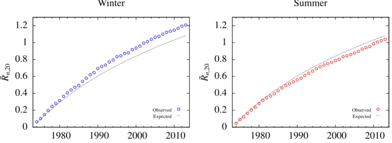
To minimize the confounding inuence of the rain probability p , k in eq. 1.11 can be raised. E.g. for Germany it was found, that the confounding inuence can be negligible for k = 20 [von Bomhard (2014)]:

R ˜

=

n

X

k=20

1 k

1 − (1 − p)

≈

n

X

k=20

1

k . (1.12)

16

0 0.2 0.4 0.6 0.8 1 1.2

1980 1990 2000 2010

˜ R

Winter

Observed Expected

0 0.2 0.4 0.6 0.8 1 1.2

1980 1990 2000 2010

˜ R

Summer

Observed Expected

Figure 1: Abbildungstext

Figure 1.2.: Additional mean records R ˜

since 1974 based on time series for the years 19542013 for the winter (left) and summer (right) seasons. Dot- ted lines show the prediction for a stationary climate and circles show the observations.

This modied mean record number R ˜

is the number of additional records from entry k = 20 to the n th step in a time series of length n . For example, the number of additional records (modied mean record number R ˜

) in a stationary climate (i.i.d. case) is expected to be 1.08 for the last 40 years of a time series of 60 years. In- terestingly, von Bomhard (2014) counted 1.25 additional daily precipitation records since 1974 in the winter seasons from 1954 to 2013 and in the summer seasons just 1.02 additional records were observed (see Fig. 1.2).

So far, there are not many more studies in the context of precipitation records.

One very recent study used both a statistical- as well as a dynamical model to show that there is a high chance for new record highs of rainfall totals in winter months in the UK under current climate conditions [Thompson et al. (2017)]. Another re- cent paper used gridded data of monthly 1-day precipitation amounts to relate an increase in record-breaking rainfall events of 12% over 19812010 to global warming [Lehmann et al. (2015)]. However, no abnormalities in daily precipitation records of stations in Scandinavia were found by Benestad (2003). Interestingly, Benestad (2003) also used the same stations for an investigation of daily temperature records.

Though he found an increase in daily temperature records, he was unable to prove a signicant trend. Indeed, other studies also failed in a proof of increasing temper- ature records [e.g. Redner and Petersen (2006)] although a global warming of 0.85

◦

C is observed since 1880 [Stocker et al. (2013)]. Only since 2009 the rst studies demonstrated a signicant trend in temperature records [Wergen and Krug (2010);

Meehl et al. (2009)]. Wergen and Krug (2010) observed a signicant increase of

17

upper temperature records. For the year 2005 they found an increase of about 40%

in temperature records registered at European stations compared to the period of 1976 to 2005. By using a linear drift model (LDM) they concluded that this increase is due to climate change.

The rst study of a LDM was published by Ballerini and Resnick [Ballerini and Resnick (1985, 1987)]. They considered a model with i.i.d. RV's X

being exposed to a linear drift of the form cn :

Y

= X

+ cn, n ≥ 1. (1.13)

Where c is a positive constant ( c > 0 ). The RV's Y

on the left hand side of eq. 1.13 are no longer identically distributed. The LDM, therefor, depends on the distribu- tions of the RV's. A detailed discussion of the LDM for the three dierent classes of extreme value statistics Weibull, Gumble and Fréchet class is given in Franke et al. (2010).

1.3. Aim

The aim of this work is to develop a statistical precipitation model for Germany which can be used to investigate the observed dierences (to theory expectations) in the mean record number (see Fig. 1.2). In the context of precipitation records it seems highly important to simulate high precipitation amounts as close to reality as possible. Since this aspect is a major weakness of commonly used amount processes (sec. 1.1) a dierent probability distribution will be developed in this work and implemented in the model. Furthermore, the occurrence process should also be able to discriminate between the two types of precipitation (convective and stratiform).

In addition the model should not be specic to one station, as it is the case for previously developed models but valid throughout Germany. For that, the utilized precipitation data (sec. 2) is analyzed according to their dependence on topographic height (above sea level) of the station and the time of the year (sec. 3). The variable height of station and time of the year will then be used as input parameters in the model. Finally, observed changes in the precipitation pattern will be implemented in the model by linear drifts (see LDM in sec. 1.2) and the inuence on the mean record number will be investigated (chapter 4).

18

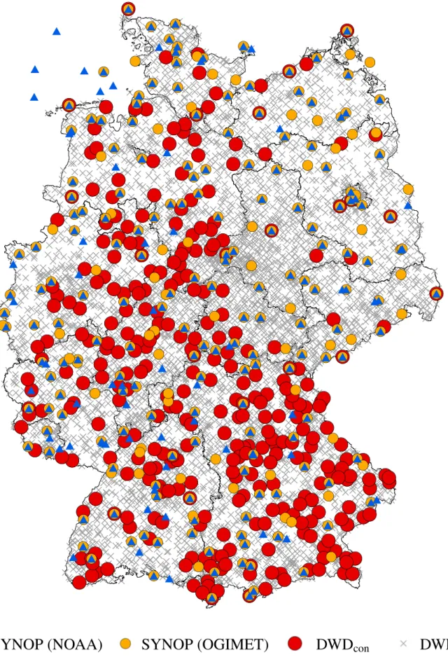
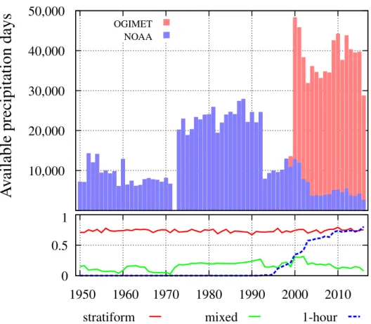
2. Data and data processing

In this work three dierent sets of data were used for analysis: Two of them are rain gauge data of the German weather service (DWD) and the third one includes SYNOP (synoptic observation data) reports. The latter one was used for disaggre- gating convective and stratiform precipitation.

The data of the DWD datasets are provided via a ftp-server

. For each station there is a separate le including the daily precipitation in mm in which 0.1mm is the minimal documented precipitation amount. The recording of precipitation was rst started at Hohenpeiÿenberg in 1781, which is the oldest meteorological mountain station worldwide [Strauch (2011)].

In the following chapter the three sets of data will be described in more detail and subsequently the processing of the data will be explained.

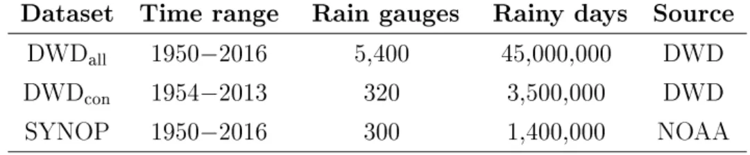
Table 2.1.: Overview of the three dierent datasets used in this study.

Dataset Time range Rain gauges Rainy days Source

DWD

1950 − 2016 5,400 45,000,000 DWD

DWD

1954 − 2013 320 3,500,000 DWD

SYNOP 1950 − 2016 300 1,400,000 NOAA

2.1. Dataset DWD all

The dataset DWD

includes all precipitation data provided by the DWD since 1950. For each station there are metadata available including the history of the rain gauge. It includes information about the elevation (above sea level) as well as the geographic longitude and latitude in decimal degrees. For the year 1901 already more than 1,400 stations are available and the precipitation network reached its peak with 4,500 stations in the 1980s [Kaspar et al. (2013)]. In total the ftp-server

1Available online: ftp-cdc.dwd.de.

19