Characterization of the submesoscale energy cascade in the Alboran Sea thermocline from spectral analysis of high-resolution MCS data
Valenti Sallares1, Jhon F. Mojica1, Berta Biescas2, Dirk Klaeschen3, and Eulàlia Gràcia1
1Barcelona-CSI, Institute of Marine Sciences - CSIC, Barcelona, Spain,2Istituto di Scienze Marine - CNR, Bologna, Italy,
3GEOMAR Helmholtz Centre for Ocean Research Kiel, Kiel, Germany
Abstract
Part of the kinetic energy that maintains ocean circulation cascades down to small scales until it is dissipated through mixing. While most steps of this downward energy cascade are well understood, an observational gap exists at horizontal scales of 103–101m that prevents characterizing a key step in the chain:the transition from anisotropic internal wave motions to isotropic turbulence. Here we show that this observational gap can be covered using high-resolution multichannel seismic (HR-MCS) data. Spectral analysis of acoustic reflectors imaged in the Alboran Sea thermocline shows that this transition is likely caused by shear instabilities. In particular, we show that the averaged horizontal wave number spectra of the reflectors vertical displacements display three subranges that reproduce theoretical spectral slopes of internal waves (λx>100 m), Kelvin-Helmholtz-type shear instabilities (100 m>λx>33 m), and turbulence (λx<33 m), indicating that the whole chain of events is occurring continuously and simultaneously in the surveyed area.
1. Introduction
Ocean kinetic energy is injected in the ocean at the production range by means of the Coriolis force, atmospheric forcing, and tides (Figure S1 in the supporting information). In a frequency (f) spectrum representation, this sub- range represents ocean motions above the Coriolis frequency (fc), where the main kinematic effect corresponds to the large-scale, geostrophically balanced eddyfield. At higher frequencies, motions are described by the mesos- cale gravity wave dynamics (Figure S1a), with most energy carried by large-amplitude, near-inertial waves off≈fc [Thorpe, 2005;Müller et al., 2005;Ferrari and Wunsch, 2009]. As they propagate through the ocean, the internal waves transfer their energy to smaller scales through an internal wave continuum driven by scattering and wave-wave interaction processes [Thorpe, 1987;Baines and Mitsudera, 1994]. These processes are thought to continue until the waves reach the buoyancy frequency (N), beyond which they become unstable [McComas and Bretherton, 1979;D’Asaro and Lien, 2000;Carnevale et al., 2001]. Finally, motions atf>Nare dominated by small-scale turbu- lence that follows isotropic internal wave breaking and leads to anisotropic irreversible mixing [e.g.,Thorpe, 2005].
While the physics that govern the internal waves and turbulent subranges is now well established, the mechanisms of energy transfer remain poorly understood. The main reason is the lack of observational sys- tems providing synoptic ocean observations in the horizontal direction at the ~103–101m range, which is the scale at which the transition between the isotropic internal waves and anisotropic turbulence occurs [e.g., Müller et al., 2005]. Theoretical knowledge suggests that the downscale energy cascade at this scale range is driven by internal wave breaking [Thorpe, 1987;Baines and Mitsudera, 1994;Riley and Lindborg, 2008].
Although different scenarios have been proposed to characterize this transition (Figure S1b), the scarce observational evidence favoring one or another makes discussions rather speculative. The fact that the cas- cade is intermittent in time and localized in space contributes to worsen the situation.
Consequently, mixing and dissipation are not formally incorporated in numerical ocean circulation models, but they are parameterized using eddy viscosity coefficients that are tuned a posteriori byfitting calculations with observations [e.g.,Gregg, 1987;Ferrari and Wunsch, 2009]. This situation hampers the predictive capabil- ity of ocean circulation models for a number of phenomena, because a significant part of heat and salt mix- ing, which affect critically long-term climate evolution or nutrient and pollutant dispersion, occurs at these scales. Therefore, there is ample agreement on the fact that afirst step toward improving model predictions is acquiring empirical knowledge on the mechanisms driving internal wave breaking and dissipation.
PUBLICATIONS
Geophysical Research Letters
RESEARCH LETTER
10.1002/2016GL069782
Key Points:
•High resolution seismic data allow characterizing ocean dynamics at the submesoscale
•Spectral slopes display a transitional subrange between internal waves and turbulence
•The transition is likely driven by shear instabilities of the Kelvin-Helmholtz type
Supporting Information:
•Supporting Information S1
Correspondence to:
V. Sallares, vsallares@icm.csic.es
Citation:
Sallares, V., J. F. Mojica, B. Biescas, D.
Klaeschen, and E. Gràcia (2016), Characterization of the submesoscale energy cascade in the Alboran Sea thermocline from spectral analysis of high-resolution MCS data,Geophys. Res.
Lett.,43, 6461–6468, doi:10.1002/
2016GL069782.
Received 27 MAY 2016 Accepted 2 JUN 2016
Accepted article online 5 JUN 2016 Published online 25 JUN 2016
©2016. American Geophysical Union.
All Rights Reserved.
In this work, we present observational evidence indicating that the energy cascade in the Alboran Sea ther- mocline appears to follow the inertia-gravity-wave route, in which internal wave breaking is likely caused by Kelvin-Helmholtz (KH)-like shear instabilities. Ourfinding is based on the analysis of the horizontal wave num- ber (kx) spectra of the vertical displacements of acoustic reflectors corresponding to isopycnal surfaces imaged with a multiscale high-resolution multichannel seismic (HR-MCS) system. In the rest of the manu- script, wefirst describe the characteristics of the acquisition system and the methods used to process and analyze the data, then we discuss the obtained results and we draw some general conclusions.
2. Study Area and Data Acquisition System
The Alboran Sea is located in the westernmost Mediterranean. It is an oceanographically active area characterized by the exchange between Atlantic and Mediterranean waters across the Strait of Gibraltar (AW and MW, respec- tively, in Figure 1). The water exchange creates a thermohaline stratification that, at the time of the HR-MCS data acquisition, was concentrated between 35 m and 110 m deep (AMW in Figure 1b). This stratified thermocline is known to be disturbed by internal waves mainly generated by barotropic tidal currents in the Strait of Gibraltar [Bruno et al., 2006; Vázquez et al., 2008] which then propagate into the Alboran basin, being scattered and reflected at the surrounding continental margins until they eventually break and dissipate. [e.g.,Global Ocean Associates, Office of Naval Research, 2002]. This situation, with the presence of a stratified and strongly sheared thermocline that is perturbed by internal waves, is theoretically prone to the development of different types of instabilities and stratified turbulence [Gregg, 1987]. The occurrence of either shear-type or convective instabil- ity depends critically on the thickness of the sheared layer. Shear instability takes place for waves with thinner interfaces, whereas convective instability dominates for waves with thick interfaces [Fringer and Street, 2003;
Troy and Koseff, 2005]. In particular, KH instabilities could develop when the interface is thin and shearing is strong enough or stratification is weak enough to bring the Richardson number, Ri= N2/|∂V/∂z|2, where N is the buoyancy frequency and∂V/∂zis the variance of the vertical shear of the horizontalflow, below a critical value of 0.25 [Thorpe, 2005]. To calculateRiwithin the targeted depth range of the Alboran AMW (30–110 m), we useN zð Þ ¼gρ0∂ρ∂zð Þz12
, wheregis gravitational acceleration,ρ0is the mean density, and∂ρ(z)/∂zis the density gradient obtained from one XCTD (eXpendable Conductivity Temperature Depth probe, see Figure 1 for loca- tion); and∂V/∂zis estimated from local ADCP (acoustic Doppler current profiler) data, which unfortunately are not simultaneous to the XCTD acquisition (SAGAS survey). The obtained value isRi= 0.2 ± 0.1, so below the critical value (see additional details in Table S1 and Figure S7). The combination of a set of conditions that are potentially prone to produce internal waves and wave instabilities, and an observational system with the appropriate Figure 1.(a) Bathymetric map of the Alboran Sea and location of the data used in the study: HR-MCS profiles acquired during the IMPULS-2006 experiment (yellow lines labeled I2 and I3), expendable bathythermograph (XBTs) profilers (red circles), expendable conductivity/temperature/depth (XCTD) probe (green circle). Sketch of the different water masses in the study region and their relative motion. Abbreviations are as follows: Atlantic Water (AW), Atlantic Modified Water (AMW), and Mediterranean Water (MW). Blue circles indicate transition depths. (b) Temperature-salinity diagram is from the XCTD probe;σ0is potential density in kg/m3. The dashed rectangle indicates the zoomed area in the inset.
Geophysical Research Letters
10.1002/2016GL069782resolution to resolve the horizontal spectrum, represents an extraordinary opportunity to identify and character- ize the whole chain of events that allows transferring the energy between internal waves and turbulence.
The two HR-MCS profiles used in this work were acquired onboard the Spanish R/V Hespérides between 16 and 19 May 2006, as part of the IMPULS (South Iberian Margin Paleoseismological Integrated Study of Large Active Structures) experiment. The characteristics of the acquisition system used in this experiment are described in Text S1 in the supporting information. MCS systems are widely used in solid earth exploration and research, and they started to be used in oceanography following the preliminary results ofGonella and Michon[1988]
and the seminal work ofHolbrook et al.[2003], which opened a new branch in operational oceanography that has been called“seismic oceanography.”Subsequently, a series of studies have demonstrated the potential of conventional MCS data to image the thermohalinefine structure of the oceans [Biescas et al., 2008;Buffett et al., 2009;Sheen et al., 2012;Ménesguen et al., 2012], to extract water properties such as sound speed, temperature, or salinity [Papenberg et al., 2010;Bornstein et al., 2013;Biescas et al., 2014;Padhi et al., 2015] or to provide infor- mation on internal wave dynamics and turbulence [Holbrook and Fer, 2005;Sheen et al., 2009;Krahmann et al., 2008;Falder et al., 2016], all with extraordinary detail in the horizontal dimension.
3. Data Processing and Analysis
3.1. MCS Data Processing
A processingflow specially designed to image the structure around the thermocline depth was applied to the HR-MCS IMPULS-2 and IMPULS-3 profiles (I2 and I3 in Figure 1a), using SEISMOS/Western-Schlumberger and Seismic Unix software. It includes 2-D geometry correction, CMP fold doubling to enhance signal-to-noise ratio (SNR), zero-phase band-pass frequencyfiltering between 40 Hz and 240 Hz to remove random back- ground noise, amplitude correction to account for geometrical spreading, prestack time migration, applica- tion of a Karhunen-Loève transformfilter with an eigenvalue cutoff ratio of 0.2 to mitigate direct wave amplitude, CMP sorting, normal move out correction, CMP stack, andfinally, poststack depth conversion using the sound speed profile measured with expendable bathythermograph (XBTs) that were deployed simultaneously to the seismic acquisition (Figure S2). The processed and depth-converted images corre- sponding to both profiles are shown in Figure 2. The seismic image is noisier for IMPULS-2. This is due to the faster shooting rate in IMPULS-2 (6 s between shots) than in IMPULS-3 (10 s), which means that coherent residual noise within the water layer arising from previous shots is higher.
3.2. Acoustic Reflectors Tracking
Despite the background noise, both profiles show clear, laterally continuous acoustic reflections within the depth range of the stratified thermocline (Figure 2). These reflectors are originated at the acoustic impedance Figure 2.Seismic record sections corresponding to HR-MCS profiles (a) IMPULS-3 and (b) IMPULS-2 (I3 and I2, respectively, in Figure 1a). The data have been processed to improve shallow water imaging and depth converted using an XBT-derived sound speed model (Figure S2). The red and blue lines correspond to the two tracked horizons analyzed in Figure 4.
Geophysical Research Letters
10.1002/2016GL069782contrasts that characterize the thermocline, essentially through temperature changes [Sallares et al., 2009]. As is explained in Text S2 in the supporting information, lateral correlation-based SNR analysis confirms that the usable frequency band to track reflectors is 40–240 Hz (Figures S3 and S4 and Table S2). A total of 117 reflec- tors with lateral correlation lengths≥1250 m were selected and automatically tracked using a criterion of maximum cross correlation between adjacent traces (Figure S5), ensuring that all of them contribute equally to the slope spectra within the analyzed scale range. The depth range of the tracked reflectors in the two pro- files is 30–100 m. Considering that lateral resolution of the HR-MCS system at the target’s depth, which is lim- ited by the width of thefirst Fresnel zone, 2Rx≈(λd)1/2, wheredis the source-target distance andλis the source wavelength, is 8–17 m (see additional details in Table S1 and Text S3 in the supporting information);
this data set provides continuous spectral coverage between 101m and 103m in the horizontal dimension.
3.3. Calculation of thekxSpectra
Figure 3 displays thekxspectra of the averaged vertical displacements of all the tracked reflectors, with their 95%
confidence intervals (2σ). The approach to calculate the spectra is analogous to that followed in previous studies [Holbrook and Fer, 2005;Sheen et al., 2009;Holbrook et al., 2013], but we use a higher-frequency source and focus on shallower targets, so lateral resolution improves. The individual power spectra of the tracked reflectors were calculated using the Fast Fourier Transform function of MATLAB, and they were normalized by the number of points. Then the average spectrum of all reflectors was calculated; it was multiplied by (2πkx)2to emphasize slope variations and scaled by the buoyancy frequency (N/N0). As suggested byHolbrook et al.[2013], we also calculated the slope spectrum directly from the seismic data. The resulting spectrum shows the same three spectral slopes at the same scales, although the slope changes are slightly more subdued. Random noise is identified at the highest wave numbers. Akxfilter (stop band) was applied to remove the harmonic noise in each profile according to the shot distance, which is 15 m (66.67 km1) for IMPULS-2 and 25 m (40 km1) for IMPULS-3 (Figure S4).
4. Discussion of Results
A key assumption when comparing the slope spectrum of vertical displacements with theoretical estimates of kinetic energy is that the undulation of acoustic reflectors reproduces indeed isopycnal displacements.
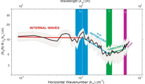
Figure 3.Average horizontal spectrum of the vertical displacement of the 117 tracked reflectors (φRx) scaled by the local buoyancy frequency at the reflector depth (N0/N) to eliminate stratification effects and multiplied by (2πkx)2to enhance slope variations (black line) and its 95% confidence interval (grey shaded area). The reference lines follow theoretical slopes of Garrett-Munk internal wave (IW) model [Garrett and Munk, 1979] (red line), Kelvin-Helmholtz instabilities [Waite, 2011]
(blue line), and Batchelor’s model for turbulence [Batchelor, 1959] (green line). The violet line is white noise. The blue rec- tangle marks the slope change between IWs and KH subranges, whereas the dashed white line labeledlNindicates the horizontal buoyancy scale calculated from oceanographic data (Table S1 and Text S5). The green rectangle labeledls indicates the limit between transitional and turbulent subranges, and the violet one labeledlnmarks the incidence of noise.
The width of these rectangles indicates the uncertainty in the determination of the slope change (i.e., the standard deviation of the slope change determined in all the individual horizons).
Geophysical Research Letters
10.1002/2016GL069782This assumption is reasonable in regions that are not subject to salinity-temperature compensating intrusions [Biescas et al., 2014], as is the case of the Alboran thermocline. It is worth noting that the spectra of the two individual profiles show the same characteristics as the combined one (Figure S4), despite the fact that the vessel moved in opposite directions during the data acquisition and that the time lapse between them was 10 h. Therefore, it must reflect robust oceanographic features that are common in the two profiles, with negligible effects of water and vessel’s motion [Klaeschen et al., 2009;Vsemirnova et al., 2009] and the images can be considered as quasi-synoptic for the scale range analyzed (Text S4).
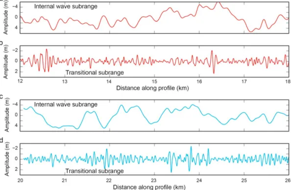
Overall, the obtainedkxspectrum displays three well-defined subranges characterized by contrasting spectral slopes (Figure 3). At the largest wavelengths of the analyzed scale range (1000 m>λx>100 m, whereλx=kx1), the energy decay follows a power law spectral density fall,kxq, withq= 2.05 ± 0.06, which corresponds to the red line in Figure 3. The obtained slope coincides with the value predicted by the Garrett-Munk heuristic internal wave model (q= 2) [Garrett and Munk, 1979], which has been observationally confirmed in a wide range of ocea- nic settings. Assuming Taylor’s hypothesis, which allows relating temporal to spatialfluctuations in turbulent flows [Taylor, 1938], the horizontal scales corresponding to the localfcandN, which define the limits of the inter- nal wave subrange, arelc=2πΔV/fc≈9.2 km andlN=2πΔV/N≈91 ± 20 m, respectively; wherefcis the Coriolis frequency at 36°,Nis the buoyancy frequency as defined in section 2, andΔVis the root-mean-square ampli- tude of the velocityfluctuation about the mean, which is also calculated within the targeted depth range (30–110 m) from the ADCP data (see additional details in Table S1 and Text S5). Interestingly, the slope change occurs at a scale that coincides—within error bounds—with the estimatedlN(Figure 3), upholding the idea that this scale actually limits the subrange controlled by gravity wave dynamics, in which most energy is carried by large amplitude, long-wavelength internal waves. To visualize the features that contribute to this part of the spectrum, we have band-passfiltered between 5000 m and 100 m the two horizons highlighted in red and blue in Figure 2. The resulting structures (Figures 4a and 4c) are compatible with IWs, having amplitudes that range from ~10 m for the largest ones (λx>103m) to a few meters for the smallest ones (λx≈lN).
The observational gap is particularly pronounced belowlN, so the knowledge on the processes governing the transition between anisotropic and isotropic motions that must occur at this scale is not based on observations.
Figure 4.Band-passfiltered reflectors corresponding to the red and blue horizons highlighted in Figure 2. (a, c) Signal has beenfiltered between 5000 m and 100 m, which correspond to the IW subrange in Figure 3. (b, d) Signal has beenfiltered between 100 m and 30 m, which correspond to the transitional subrange (KH instabilities in Figure 3).
Geophysical Research Letters
10.1002/2016GL069782Theory and models indicate that the transitional subrange associated to KH-instabilities and stratified turbulence should display a spectral roll-off nearlN, marking the point where dissipative effects overcome the stability that dominates at larger scales [Gregg, 1987;D’Asaro and Lien, 2000;Carnevale et al., 2001]. In particular, high- resolution numerical experiments give aqvalue of 2.5–3.1 [Waite, 2011]. This is consistent with the spectral slope ofq= 2.8 ± 0.2 obtained betweenlNandls≈33 ± 4 m from the tracked horizons (Figure 3). The features that con- tribute to this spectral subrange for the blue and red horizons of Figure 2 are shown in Figures 4b and 4d.
The likely presence of KH billows in the Mediterranean thermocline wasfirst shown by dye tracing experiments performed around Malta [Woods, 1968]. However, one of the clearest recent observational evidence corre- sponds to a KH billow train imaged with a thermistor chain in a downslope tidalflow above the sloping side of the Great Meteor Seamount, Canary Basin [van Haren and Gostiaux, 2010;Smyth and Moum, 2012]. These data show a rough, wavy horizon displaying a series of spikes with amplitudes of 1–5 m and wavelengths of 50–75 m.
Even if both the depth and oceanographic setting of this experiment differs from ours, it is worth noting that the features identified as KH billows are consistent with those contributing to the transitional subrange in our data (Figures 4b and 4d). Another distinctive hallmark of KH billows is a wavelength,l, 1 order of magnitude larger than the thickness of the sheared layer,δ, which marks in turn the maximum size of the fastest growing distur- bances [e.g.,Smyth and Moum, 2012]. Our observations suggest a rather complex situation, certainly more than in lab and numerical experiments. First, the transitional subrange, which we interpret to represent KH billows (Figure 4), covers a range of scales—hence possible values ofl—between ~100 m and ~30 m. Second, the thick- ness of the sheared layers, as defined by the vertical separation between contiguous reflectors, is also variable (δ= 13 ± 3 m). If we assume that the point of slope breaking toward the transitional domain (λx≈100 ± 20 m) marks the wavelength of the greatest disturbances, we obtainl/δ= 100/13≈7.5, similar to what was originally described for KH billows in a steadyflow [Miles and Howard, 1964]. However, the range of possible values for bothδandlprevents any general interpretation or conclusion concerning the value ofl/δ. Similarly, it has been shown that the prevalence of KH-type instability depends critically valuekδ, wherek = 2π/λandλis the wave- length of the internal wave [Fringer and Street, 2003]. Whenkδ<0.56, the most unstable wavelength associated with a shear instability is small enough to grow at the interface and develop KH billows, but it is not energetic enough to induce convective instability. For the values described above, we obtainkδ<0.5, providing addi- tional support to the presence of KH instabilities. However, as in the case ofl/δ, there is a range of possible values forkandδthat makes difficult a direct, univocal comparison with experimental results.
While the onset of KH-instabilities atlNis reproduced by numerical simulations, the scale of transition to tur- bulence is unclear. In the obtained spectrum, the slope changes toq≈1.64 atls≈33 ± 4 m (Figure 3). This slope is close to theq= 5/3 predicted by the Batchelor’s model [Batchelor, 1959], which describes the energy continuum of the turbulent inertial subrange. This coincidence suggests that the smallest billows have col- lapsed, and dynamics starts to be dominated by turbulence atls. This scale is 1 order of magnitude larger than the local Ozmidov length scale,lo≈2 ± 1 m (Table S1 and Text S5), suggesting that the transition does not reflect the transition to isotropic turbulence but rather to stratified turbulence. The smallest scale that is resolved with the HR-MCS system, as indicated by the slope change toq≈0, characteristic of white noise, isln≈15 m (Figure 3), a value consistent with the nominal lateral resolution of the system (Table S1).
In summary, the spectral analysis of the multiscale HR-MCS data allows characterizing the sequence of events that drives the energy cascade between internal waves and turbulence in the Mediterranean thermocline.
Our interpretation is that transition starts with the development of KH instabilities, whichfirst capture the internal wave energy along the stratified thermocline nearlN, and then they transfer it to the turbulent scale after collapsing nearls. Even though our analysis is local, the fact that the averaged spectrum displays the transitional subrange indicates that KH billows are ubiquitous in the area, so this chain of events is taking place continuously and simultaneously, with each process occurring at and affecting to a specific scale range.
As stated in the introduction, current knowledge on the mechanisms governing the energy transfer at the submesoscale is rather poor mainly due to the lack of observational systems providing observations at the appropriate range of scales. This makes that small-scale phenomena are not formally incorporated in numer- ical ocean circulation models, hindering their predictive capability in scenarios where mixing and dissipation are important. The availability of an observational system that can cover this observational gap could possibly help mitigating this issue. Additionally, it must be noted that in contrast to the conventional heavy,fixed, limited-resolution MCS systems used in previous experiments, the HR-MCS ones are relatively light and
Geophysical Research Letters
10.1002/2016GL069782portable, so they can be readily installed and operated in middle-sized oceanographic vessels. This fact, com- bined with the better resolution that provides the higher-frequency source, opens new perspectives in ocea- nographic research at the submesoscale.
5. Conclusions
The spectral analysis of the vertical displacements of acoustic reflectors at thermohaline boundaries using data acquired with a multiscale, HR-MCS system provides observational evidence indicating that the energy cascade between mesoscale and small-scale motions in the Alboran Sea thermocline is driven by the devel- opment of internal wave shear instabilities of the Kelvin-Helmholtz type. In particular, our results show that ocean dynamics at the thermocline depth is dominated by internal waves at scales larger than the horizontal buoyancy scale,lN≈91 m, below which shear instabilities of the KH type develop until they collapse at ls≈33 m, giving rise to turbulence. These observations shed new light on the mechanisms and routes of energy transfer between internal waves and turbulence in the thermocline. Even if our study is local, the avail- ability of a relatively light, portable system providing observations at the appropriate scales opens new per- spectives to improve our knowledge on mixing and dissipation.
References
Baines, P., and H. Mitsudera (1994), On the mechanism of shearflow instabilities,J. Fluid Mech.,276, 327–342.
Batchelor, G. K. (1959), Small-scale variation of convected quantities like temperature in turbulentfluid,J. Fluid Mech.,5, 113–139.
Biescas, B., V. Sallares, J. L. Pelegrí, F. Machin, R. Carbonell, G. Buffett, J. J. Dañobeitia, and A. Calahorrano (2008), Imaging meddyfinestructure using multichannel seismic reflection data,Geophys. Res. Lett.,35, L11609, doi:10.1029/2008GL033971.
Biescas, B., B. R. Ruddick, M. R. Nedimovic, V. Sallarès, G. Bornstein, and J. F. Mojica (2014), Recovery of temperature, salinity and potential density from ocean reflectivity,J. Geophys. Res. Oceans,119, 3171–3184, doi:10.1002/2013JC009662.
Bornstein, G., B. Biescas, V. Sallares, and J. F. Mojica (2013), Direct temperature and salinity acoustic full waveform inversion,Geophys. Res.
Lett.,40, 4344–4348, doi:10.1002/grl.50844.
Bruno, M., A. Vázquez, J. Gómez-Enri, J. M. Vargas, J. García Lafuente, A. Ruiz-Cañavate, L. Mariscal, and J. Vidal (2006), Observations of internal waves and associated mixing phenomena in the Portimao Canyon area,Deep Sea Res., Part II,53, 1,219–1,240.
Buffett, G., B. Biescas, J. L. Pelegrí, F. Machín, V. Sallares, R. Carbonell, D. Klaeschen, and R. Hobbs (2009), Seismic reflection along the path of the Mediterranean undercurrent,Cont. Shelf Res.,29, 1848–1860.
Carnevale, G. F., M. Briscolini, and P. Orlandi (2001), Buoyancy- to inertial-range transition in forced stratified turbulence,J. Fluid Mech.,427, 205–239.
D’Asaro, E. A., and R. C. Lien (2000), Lagrangian measurements of waves and turbulence in stratifiedflows,J. Phys. Oceanogr.,30, 641–655.
Falder, M., N. J. White, and C. P. Caufield (2016), Seismic imaging of rapid onset of stratified turbulence in the South Atlantic ocean,J. Phys.
Ocean.,46, 1023–1044, doi:10.1175/JPO-D-15-0140.1.
Ferrari, R., and C. Wunsch (2009), Ocean circulation kinetic energy: Reservoirs, sources and sinks,Annu. Rev. Fluid Mech.,41, 253–282, doi:10.1146/annurev.fluid.40.111406.102139.
Fringer, O. B., and R. L. Street (2003), The dynamics of breaking progressive interfacial waves,J. Fluid Mech.,494, 319–353, doi:10.1017/
S0022112003006189.
Garrett, C., and W. Munk (1979), Internal waves in the ocean,Annu. Rev. Fluid Mech.,11, 339–369.
Global Ocean Associates, Office of Naval Research (2002), An Atlas of oceanic internal solitary wave; The Strait of Gibraltar, Code 322PO.
[Available at http://www.internalwaveatlas.com/Atlas_PDF/IWAtlas_Pg099_StraitGibraltar.PDF.]
Gonella, J., and D. Michon (1988), Deep internal waves measured by seismic reflection within the eastern Atlantic water column,C. R. Acad.
Sci. Ser. II,306, 781–787.
Gregg, M. C. (1987), Diapycnal mixing in the thermocline: A review,J. Geophys. Res.,92, 5,249–5,286, doi:10.1029/JC092iC05p05249.
Holbrook, W. S., and I. Fer (2005), Ocean internal wave spectra inferred from seismic reflection transects,Geophys. Res. Lett.,32, L15604, doi:10.1029/2005GL023733.
Holbrook, W. S., P. Páramo, S. Pearse, and R. W. Schmitt (2003), Thermohalinefine structure in an oceanographic front from seismic reflection profiling,Science,301, 821–824.
Holbrook, W. S., I. Fer, R. W. Schmitt, D. Lizarralde, J. M. Klymak, L. C. Helfrich, and R. Kubichek (2013), Estimating oceanic turbulence dissi- pation from seismic images,J. Atmos. Oceanic Technol.,30, 1767–1788.
Klaeschen, D., R. W. Hobbs, G. Krahmann, C. Papenberg, and E. Vsemirnova (2009), Estimating movement of reflectors in the water column using seismic oceanography,Geophys. Res. Lett.,36, L00D03, doi:10.1029/2009GL038973.
Krahmann, G., P. Brandt, D. Klaeschen, and T. Reston (2008), Mid-depth internal wave energy off the Iberian Peninsula estimated from seismic reflection data,J. Geophys. Res.,113, C12016, doi:10.1029/2007JC004678.
McComas, C. H., and F. P. Bretherton (1977), Resonant interaction of oceanic internal waves,J. Geophys. Res.,82(9), 1397–1412, doi:10.1029/
JC082i009p01397.
McComas, C. H., and F. P. Bretherton (1979), Resonant interaction of oceanic internal waves,J. Geophys. Res.,82, 1397–412, doi:10.1029/
JC082i009p01397.
Ménesguen, C., B. Hua, X. Carton, F. Klingelhoefer, P. Schnurle, and C. Reichert (2012), Arms winding around a meddy seen in seismic reflection data close to the Morocco coastline,Geophys. Res. Lett.,39, L05604, doi:10.1029/2011GL050798.
Miles, J. W., and L. N. Howard (1964), Note on a heterogeneous shearflow,J. Fluid Mech.,20, 331–336, doi:10.1017/S0022112064001252.
Müller, P., J. McWilliams, and M. Molemaker (2005), Routes to dissipation in the ocean: The two-dimensional/three-dimensional turbulence conundrum, inMarine Turbulence, Observations and Models. Results of the CARTUM project, edited by H. Z. Baumert, J. Simpson, and J.
Sündermann, Cambridge Univ. Press, Cambridge, U. K.
Padhi, A., S. Mallick, W. Fortin, W. S. Holbrook, and T. Blacic (2015), 2-D ocean temperature and salinity images from pre-stack seismic waveform inversion methods: An example from the South China Sea,Geophys. J. Int.,202(2), 800–810, doi:10.1093/gji/ggv188.
Geophysical Research Letters
10.1002/2016GL069782Acknowledgments
We thank J.L. Pelegrí and P. Puig for reading early versions of the manu- script, M. Bruno for critical review of the work, and all colleagues at Barcelona- CSI for advice and support. Data are available under request to thefirst author. This work has been done in the framework of projects POSEIDON (CTM2010-25169) and APOGEO (CTM2011-16001-E/MAR), both funded by the Spanish MINECO. The seismic and oceanographic data were acquired during the IMPULS (CTM2003-05996- MAR) and SAGAS (CTM2005-08071-C03- 02/MAR) surveys also from MINECO.
Third author’s work has been supported by the European Commission through OCEANSEIS project (Marie Curie Action FP7-PEOPLE-2010-IOF-271936) and Marie Curie Action FP7-PEOPLE-2012- COFUND-600407.
Papenberg, C., D. Klaeschen, G. Krahmann, and R. Hobbs (2010), Ocean temperature and salinity inverted from combined hydrographic and seismic data,Geophys. Res. Lett.,37, L04601, doi:10.1029/2010GL042115.
Riley, J., and E. Lindborg (2008), Stratified turbulence: A possible interpretation of some geophysical turbulence measurements,J. Atmos. Sci., 65, 2,416–2,424.
Sallares, V., B. Biescas, G. Buffett, R. Carbonell, J. J. Dañobeitia, and J. L. Pelegrí (2009), Relative contribution of temperature and salinity to ocean acoustic reflectivity,Geophys. Res. Lett.,36, L00D06, doi:10.1029/2009GL040187.
Sheen, K. L., N. J. White, and R. W. Hobbs (2009), Estimating mixing rates from seismic images of oceanic structure,Geophys. Res. Lett.,36, L00D04, doi:10.1029/2009GL040106.
Sheen, K. L., N. J. White, C. P. Caulfield, and R. W. Hobbs (2012), Seismic imaging of a large horizontal vortex at abyssal depths beneath the sub-Antarctic front,Nat. Geosci.,5, 542–546, doi:10.1038/ngeo1502.
Smyth, W., and J. Moum (2012), Ocean mixing by Kelvin-Helmholtz instability,Oceanography,25, 140–148.
Taylor, G. I. (1938), The spectrum of turbulence,Proc. R. Soc. London A,164, 476.
Thorpe, S. A. (1987), Transition phenomena and the development of turbulence in stratifiedfluids,J. Geophys. Res.,92, 5,231–5,245, doi:10.1029/JC092iC05p05231.
Thorpe, S. A. (2005),The Turbulent Ocean, Cambridge Univ. Press, Cambridge, U. K.
Troy, C. D., and J. R. Koseff (2005), The instability and breaking of long internal waves,J. Fluid Mech.,543, 107–136, doi:10.1017/
S0022112005006798.
Van Haren, H., and L. Gostiaux (2010), A deep-ocean Kelvin-Helmholtz billow train,Geophys. Res. Lett.,37, L03605, doi:10.1029/
2009GL041890.
Vázquez, A., M. Bruno, A. Izquierdo, D. Macias, and A. Ruiz-Cañavate (2008), Meteorologically forced subinertialflows and internal wave generation at the main sill of the strait of Gibraltar,Deep Sea Res. I,55, 1,277–1,283.
Vsemirnova, E., R. Hobbs, N. Serra, D. Klaeschen, and E. Quentel (2009), Estimating internal wave spectra using constrained models of the dynamic ocean,Geophys. Res. Lett.,36, L00D07, doi:10.1029/2009GL039598.
Waite, M. L. (2011), Stratified turbulence at the buoyancy scale,Phys. Fluids,23, 066602.
Woods, J. (1968), Wave-induced shear instability in the summer thermocline,J. Fluid Mech.,32, 791–800.