Forecasting travel: An agent-based approach

Research Collection

Other Publication

Forecasting travel

An agent-based approach

Author(s):

Axhausen, Kay W.

Publication Date:

2020-02

Permanent Link:

https://doi.org/10.3929/ethz-b-000398758

Rights / License:

In Copyright - Non-Commercial Use Permitted

This page was generated automatically upon download from the ETH Zurich Research Collection. For more information please consult the Terms of use.

ETH Library

Preferred citation style

Axhausen, K.W. (2020) Forecasting travel: An agent-based approach, web-lecture, Alphabet series on “Modelling Real-World

Phenomena, February 2020.

.

Alphabet 2020

Forecasting travel: An agent-based approach

KW Axhausen IVT

ETH Zürich

February 2020

Acknowledgments - MATSim @ ETH, TU Berlin

Alphabet 2020

Prof. Kay Axhausen Dr. Milos Balac Dr. Michael Balmer Dr. Henrick Becker Dr. Joschka Bischoff Dr. David Charypar Billy Charlton Dr. Nurhan Cetin Dr. Artem Chakirov Dr. Yu Chen

Prof. Francesco Ciari Dr. Christoph Dobler Prof, Alexander Erath Ricardo Ewert

Dr. Matthias Feil Dr. Gunnar Flötteröd Dr. Pieter Fourie Dr. Christian Gloor Dr. Dominik Grether Dr. Jeremy K. Hackney Dr. Andreas Horni

Sebastian Hörl Anugrah Ilahi Dr. Ihab Kaddoura Grace Kagho Janek Laudan Nicolas Lefebvre Gregor Leich

Clarissa Livingston Dr. Johannes Illenberger Dr. Gregor Lämmel Dr. Michal Maciejewski Patrick Manser

Dr. Konrad Meister Dr. Lu Ming

Joe Molloy

Dr. Manuel Moyo Dr. Kirill Müller Sebastian Müller Prof. Kai Nagel

Dr, Andreas Neumann Dr. Thomas Nicolai

Dr. Benjamin Kickhöfer Dr. Sergio Ordonez Stefano Penazzi Dr. Bryan Raney Dr. Marcel Rieser Aurore Sallard

Dr. Nadine Schüssler Dr. Lijun Sun

Dr. David Strippgen Christopher Tchervenkov Theresa Thunig

Dr. Michael Van Eggermond

Dr. Rashid Waraich Dominik Ziemke Dr. Michael Zilske

Basic assumptions

Alphabet 2020

Basic definition

Social generalised costs is the sum of

individual generalised costs, ^i.e.

decision relevant generalised costs &

overlooked individual costs

And the

externalities caused

Alphabet 2020

Basic assumption

Traffic is a system of moving, self-organising

Queues

Alphabet 2020

Basic assumption

The crucial short-term interaction between capacity, i.e. the

number of slots

for the desired speed and the

current demand

Alphabet 2020

Basic assumption

Societies chose their

number of slots

By the

design/operation of the road/rail network

For the

desired speeds

Alphabet 2020

Basic assumption

Travel demand (pkm or tkm) is a

normal good

i.e. it grows with

decreasing individual “generalised costs”

Alphabet 2020

Basic assumption

The travellers chose their

average decision relevant generalised costs

with their package of

locations (residence, work) ^and mobility tools

Alphabet 2020

Alphabet 2020

What are the tasks ?

Alphabet 2020

Time horizons of transport planning

Horizon Examples

½ year New transit line, new timetable, new parking fees

2 years New transit network, new business park, new mall

40 years Long-term population change, new residential

patterns, new motorway networks, new railway

tracks

Alphabet 2020

Market model

For all goods i of the market:

k‘

= f(q‘

(k‘

, B

), A

)

k‘ : Estimated generalised costs [SFr/good]

q‘ : Estimated demand [Elements/Unit time]

A : Supply of the goods

B : Population (natural and legal)

t : Time t

o : Place o

g : Group g

z : Year z

Alphabet 2020

Parts of the market model

Supply side model: How do the (generalised) costs change as a function of demand given a supply (capacity) ?

k‘

= f(q‘

, A

)

Demand model: How does demand respond to the (generalised) costs given a certain population ?

q‘

= f(k‘

, B

)

Alphabet 2020

Generic model structure

Competition for slot in facilities and the network

k(t,r,j)

q

≡ (t,r,j)

β

Population

“Scenario”

Scheduling

Mental map

Key points of the critique of equilibrium approaches

• Travellers aren’t in equilibrium

• Travellers don’t know all alternatives

• Travellers don’t plan their whole day (week) in advance

Alphabet 2020

How do we label our models?

Alphabet 2020

A detour via a closed form approach for the supply model

Alphabet 2020

Acknowledgments for the detour

A Loder, IVT, ETH Zürich L Ambühl , IVT, ETH Zürich

M Menendez , IVT, ETH Zürich, but now NYU Abu Dhabi M Bliemer, University of Sydney

Alphabet 2020

Macroscopic Fundamental Diagram (MFD)

• MFDs describe road networks as a trip processing factory

• MFDs have an optimal or critical point where trip completion is maximized

• MFDs are a feature of a network NOT demand

Alphabet 2020

Empirical MFDs

Alphabet 2020

Influence of network design: Betweenness-Centrality

Loder et al. (2019). Scientific Reports (in press).Alphabet 2020

First results for multi-modal MFDs: London

Loder, Bressan, Ambühl, Bliemerand Axhausen (2018)

Alphabet 2020

How do we label our models?

Alphabet 2020

Dimensions of transport models

Resolution Agents, flows

Spatial resolution Zones, parcels, units

Scheduling model Trip, tour, daily chain (with breaks) Choice model DCM, rules&heuristics

Route choice Integrated, external (with consistent valuations?)

Choice set construction Explicit, implicit

Solution method Whole population (& MSA or similar)

Sample enumeration (& MSA or similar), co-evolutionary search

Schedule equilibrium Yes, no

Alphabet 2020

MATSim

Resolution Agents, flows

Spatial resolution Zones, parcels, units

Scheduling model Trip, tour, daily chain without breaks Choice model DCM, rules&heuristics

Route choice Integrated with consistent valuations, external Choice set construction Explicit, implicit

Solution method Whole population (& MSA or similar)

Sample enumeration (& MSA or similar), co-evolutionary search

Schedule equilibrium Yes, no

Alphabet 2020

MATSim – A GNU open source project

Alphabet 2020

MATSim: A GNU public licence software project

Main partners:

• TU Berlin (Prof. Nagel)

• ETH Zürich inc. FCL SIngapore Contributors, users, e.g.:

• Swiss Federal Railroads (SBB, Berne)

• senozon, Zürich (Dr. Balmer)

• simunto, Zürich (Dr. Rieser)

• University of Pretoria

• Transport Foundry, Atlanta

• nommon, Barcelona

• KPMG, Melbourne

• Airbus, Toulouse

Alphabet 2020

Current status

Known implementations: About 45 (Europe, Asia, US)

Research groups: About 35 (including some beyond transport)

Uses: Research

Some initial commercial uses Some policy consulting

Software: Last reimplementation in 2012/13 Stable API

Daily tests JAVA

Alphabet 2020

MATSim Status 2018

Alphabet 2020

© Marcel Rieser, simunto

© Marcel Rieser, simuunto

A model of Singapore‘s travel demand and traffic

Alphabet 2020

MATSim: Base approach

Alphabet 2020

Equilibrium search in MATSim

Simulation of

flows on networks and to facilities

k(t,r,j)

q

≡ (t,r,j)

Score (utility) calculation Initial

schedules

(Optimal) Replanning

(inc. connection)

& plan choice

U

(t,r,j)

Alphabet 2020

SUE search example

Alphabet 2020

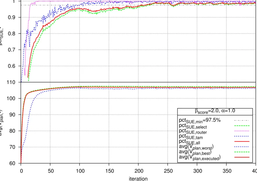
2.5. Equilibration with standard parameters

Figure 2.2: pct_SUE across the iterations with base case parameters

60 70 80 90 100 110 0.6 0.7 0.8 0.9 1

0 50 100 150 200 250 300 350 400

avg(V plan,*) pct SUE,*

iteration

β_score=2.0, α=1.0 pct_SUE,min=97.5%

pct_SUE,select pct_SUE,router pct_SUE,tam pct_SUE,all avg(V_plan,worst) avg(V_plan,best) avg(Vplan,executed)

The value ofpctSUE,min of 97.5% is chosen arbitrarily.

• The learning rate parameter ↵ is set to 1.0, meaning that the new score of a re- evaluated plan equals the score of its most recent simulation and does not depend on its previous score values. In addition to the variation of score, Section 2.6 studies how the agent based SUE condition is influenced by this parameter.

2.5.1 Results

The development ofpct_SUE across the iterations is depicted in the upper half of Fig. 2.2.

The averages of the scores of the executed plans, the worst and the best plans are dis- played in the lower half for the common visual inspection. At different numbers of iterations, pct_SUE exceeds pct_SUE,min for the various strategies, and for all agents com- bined:

• pct_SUE,all denotes the percentage of all agents combined for which the SUE con- dition is fulfilled,

• pct_SUE,select denotes this percentage of those agents who selected one of their

existing plans according to Eq. (1.2),

• pct_SUE,router and pct_SUE,tam denote the percentages of those agents who generated

the plan via replanning with the router or the time allocation mutator.

In the following a closer look is taken at the iterations in which each of the pct_SUE,⇤ exceeds pct_SUE,min. In the cases of all percentages except pct_SUE,all, the interpretation

27

Co-evolution – Issues

• Size of search space ~ Behavioural alternatives

• Rate of replanning (~ MSA)

• Size of the choice set ~ RAM

• Similarity of the daily schedules

• Integration into a log-sum term

• Stability of link/vehicle based results

Alphabet 2020

Activity schedule dimensions

Alphabet 2020

37

Activity scheduling dimensions

Number and type of activities Sequence of activities

• Start and duration of activity

• Composition of the group undertaking the activity

• Expenditure division

• Location of the activity

• Movement between sequential locations

• Location of access and egress from the mean of transport

• Parking type

• Vehicle/means of transport

• Route/service

• Group travelling together

• Expenditure division

Alphabet 2020

Current Vickrey-type utility function

å

å = -

=

+

= ⁿ

i

i i trav n

i

i act

plan U U

U

2

, 1 , 1

,

U _{act ,i} = U _{dur ,i} + U _{late. ar ,i}

Alphabet 2020

Example application: How many AV taxis can survive?

Alphabet 2020

Acknowledgments for the example

S Hörl for the work on AV simulation

F Becker for the new mode choice and mobility tool models P Bösch, F Becker and H Becker for the cost estimates

Alphabet 2020

Simulation Framework: DVRP extension

Alphabet 2020

Maciejewskiet al. (2017)

Alphabet 2020

aTaxi price and fleet size determination

Simulation

Price calculator

(Bösch et al., 2016) New price

Price adjustment Empty mileage Occupancy

Customer mileage

Results – city of Zürich only: VKT

Alphabet 2020

Challenges

Alphabet 2020

What I haven’t talked about?

• Econometric estimation/machine learning techniques

• Population synthesis and forecasting

• Residential and workplace choice

• Mobility tool ownership choices

• Travel behaviour capture and modelling

• Land market response

• Labour market response

• Network design, e.g. timetable design, network optimisation

• Technology choices, e.g. e-mobility infrastructure

Alphabet 2020

Challenges for MATSim

• Econometric estimation of the whole day scoring function

• Increase the size and variance of the implicit choice set

• Link to a log-sum formulation for welfare assessment

• Accelerating the iterative equilibrium search

• Gridlock modeling (& stability of equilibrium)

• Generation of artificial social networks in the agent- population

• Multiple agent-type equilibria

Alphabet 2020

Questions ?

www.matsim.org www.ivt.ethz.ch

www.futurecities.ethz.ch www.senozon.com

www.simunto.com

Alphabet 2020

Questions ?

Alphabet 2020

References

Alphabet 2020

References

Horni, A., K. Nagel, and K. W. Axhausen (eds.) (2016) The Multi-Agent Transport Simulation MATSim, Ubiquity, London.

Hörl, S., F. Becker, T. Dubernet und K.W. Axhausen (2019) Induzierter Verkehr durch autonome Fahrzeuge: Eine Abschätzung,

Forschungsprojekt SVI 2016/001, Schriftenreihe, 1650, UVEK, Bern Loder, A., L. Ambühl, M. Menendez and K.W. Axhausen (2017) Empirics

of multimodal traffic networks - Using the 3D macroscopic

fundamental diagram, Transportation Research Part C, 82, 88-101.

Loder, A., L. Ambühl, M. Menendez and K.W. Axhausen (2019) Understanding traffic capacity of urban networks, Scientific Reports, 9, 16283.

Alphabet 2020

Appendix

Alphabet 2020

The typical four-stage model

Resolution Agents, flows

Scheduling model Trip, tour, daily chain (with breaks) Choice model DCM, rules&heuristics

Route choice Integrated, external without consistent valuations

Choice set construction Explicit, implicit

Solution method Whole population (& MSA or similar)

Sample enumeration (& MSA or similar), co-evolutionary search

Schedule equilibrium (Yes), no

Alphabet 2020

The typical activity-based model (ABM)

Resolution Agents, flows

Scheduling model Trip, tour, daily chain (with breaks) Choice model DCM , rules&heuristics

Route choice Integrated, external without consistent valuations

Choice set construction Explicit, implicit

Solution method Whole population (& MSA or similar)

Sample enumeration (& MSA or similar), co-evolutionary search

Schedule equilibrium Yes, none reported it yet

Alphabet 2020

Following the agents

Alphabet 2020

MATSim: Logic of the co-evolution – Step 0

Agent 1

Plan 1.1 H-W-H; 8:00, 17:00; C,C;

Agent 2

Plan 2.1 H-W-H; 8:00, 17:00; C,C;

Agent 3

Plan 3.1 H-W-H; 8:00, 17:00; C,C;

Alphabet 2020

Co-evolution – Step 1.1 – Simulation/scoring

Agent 1

Plan 1.1 H-W-H; 8:00, 17:00; C,C; 35

Agent 2

Plan 2.1 H-W-H; 8:00, 17:00; C,C; 35

Agent 3

Plan 3.1 H-W-H; 8:00, 17:00; C,C; 35

Alphabet 2020

Co-evolution – Step 1.2 – After replanning (1/3)

Agent 1

Plan 1.1 H-W-H; 8:00, 17:00; C,C; 35

Agent 2

Plan 2.1 H-W-H; 8:00, 17:00; C,C; 35

Agent 3

Plan 3.1 H-W-H; 8:00, 17:00; C,C; 35 Plan 3.2 H-W-H; 8:15, 17:30; C,C

Alphabet 2020

Co-evolution – Step 1.3 – After plan selection (best/MNL)

Agent 1

Plan 1.1 H-W-H; 8:00, 17:00; C,C; 100%

Agent 2

Plan 2.1 H-W-H; 8:00, 17:00; C,C; 100%

Agent 3

Plan 3.1 H-W-H; 8:00, 17:00; C,C; 35 Plan 3.2 H-W-H; 8:15, 17:30; C,C; New

Alphabet 2020

Co-evolution – Step 2.1 – Simulation/scoring

Agent 1

Plan 1.1 H-W-H; 8:00, 17:00; C,C; 45

Agent 2

Plan 2.1 H-W-H; 8:00, 17:00; C,C; 45

Agent 3

Plan 3.1 H-W-H; 8:00, 17:00; C,C; 35 Plan 3.2 H-W-H; 8:15, 17:30; C,C; 60

Alphabet 2020

Co-evolution – Step 2.2 – After replanning (1/3)

Agent 1

Plan 1.1 H-W-H; 8:00, 17:00; C,C; 45 Plan 1.2 H-W-H; 8:00, 17:00; B,B;

Agent 2

Plan 2.1 H-W-H; 8:00, 17:00; C,C; 45 Agent 3

Plan 3.1 H-W-H; 8:00, 17:00; C,C; 35 Plan 3.2 H-W-H; 8:15, 17:30; C,C; 60

Alphabet 2020

Co-evolution – Step 2.3 – After plan selection (best/MNL)

Agent 1

Plan 1.1 H-W-H; 8:00, 17:00; C,C; 45 Plan 1.2 H-W-H; 8:00, 17:00; B,B; New

Agent 2

Plan 2.1 H-W-H; 8:00, 17:00; C,C; 100%

Agent 3

Plan 3.1 H-W-H; 8:00, 17:00; C,C; 38%

Plan 3.2 H-W-H; 8:15, 17:30; C,C; 62%

Alphabet 2020

Co-evolution – Step 3.1 – Simulation/scoring

Agent 1

Plan 1.1 H-W-H; 8:00, 17:00; C,C; 45 Plan 1.2 H-W-H; 8:00, 17:00; B,B; 70

Agent 2

Plan 2.1 H-W-H; 8:00, 17:00; C,C; 45

Agent 3

Plan 3.1 H-W-H; 8:00, 17:00; C,C; 45 Plan 3.2 H-W-H; 8:15, 17:30; C,C; 60

Alphabet 2020

Co-evolution – Step 3.2 – After replanning (1/3)

Agent 1

Plan 1.1 H-W-H; 8:00, 17:00; C,C; 45 Plan 1.2 H-W-H; 8:00, 17:00; B,B; 70 Agent 2

Plan 2.1 H-W-H; 8:00, 17:00; C,C; 45 Agent 3

Plan 3.1 H-W-H; 8:00, 17:00; C,C; 45 Plan 3.2 H-W-H; 8:15, 17:30; C,C; 60 Plan 3.3 H-W-H; 7:30, 17:15; B,B

Alphabet 2020

Co-evolution – Step 3.3 – After plan selection (best/MNL)

Agent 1

Plan 1.1 H-W-H; 8:00, 17:00; C,C; 36%

Plan 1.2 H-W-H; 8:00, 17:00; B,B; 64%

Agent 2

Plan 2.1 H-W-H; 8:00, 17:00; C,C; 100%

Agent 3

Plan 3.1 H-W-H; 8:00, 17:00; C,C; 45 Plan 3.2 H-W-H; 8:15, 17:30; C,C; 60 Plan 3.3 H-W-H; 7:30, 17:15; B,B New

(The (worst) plan, more then memory allows, is deleted)

Alphabet 2020

Co-evolution – Summary of best scores

Iteration 1 Iteration 2 Iteration 3

Agent 1 35 45 80

Agent 2 35 45 45

Agent 3 35 60 60

Mean 35 50 62

Alphabet 2020

Future whole day utility function?

Time elements linear

• Travel time By mode and type of service;

by crowding level

by comfort level (parking search, stop&go)

• Transfer penalty

• Late penalty by activity type

Activity time log (Vickrey) or S-shape (Joh) (all, individual)

• Minimum duration by activity type

• Preferred duration by activity type

• Duration by time of day (might go away if participation is included)

Destination Attractiveness, Value for money Expenditure by activity

by mode/type of service

Alphabet 2020

Updated full cost/pkm estimate (current occupancy levels)

Alphabet 2020

Updated full cost/pkm estimate (current occupancy levels)

Alphabet 2020

Fleet size determination: Stability of the process

Alphabet 2020