IHS Economics Series Working Paper 81
March 2000
Cyclical Occupational Choice in a Model with Rational Wage Expectations and Perfect Occupational Mobility
Bernhard Felderer
André Drost
Impressum Author(s):
Bernhard Felderer, André Drost Title:
Cyclical Occupational Choice in a Model with Rational Wage Expectations and Perfect Occupational Mobility
ISSN: Unspecified
2000 Institut für Höhere Studien - Institute for Advanced Studies (IHS) Josefstädter Straße 39, A-1080 Wien
E-Mail: o ce@ihs.ac.atffi Web: ww w .ihs.ac. a t
All IHS Working Papers are available online: http://irihs. ihs. ac.at/view/ihs_series/
This paper is available for download without charge at:
https://irihs.ihs.ac.at/id/eprint/1256/
Institut für Höhere Studien (IHS), Wien Institute for Advanced Studies, Vienna
Reihe Ökonomie / Economics Series No. 81
Cyclical Occupational Choice in a Model with Rational Wage Expectations and Perfect
Occupational Mobility
Bernhard Felderer, André Drost
Cyclical Occupational Choice in a Model with Rational Wage Expectations and Perfect Occupational Mobility
Bernhard Felderer, André Drost
Reihe Ökonomie / Economics Series No. 81
March 2000
Institut für Höhere Studien Stumpergasse 56, A-1060 Wien Fax: +43/1/599 91-163
Bernhard Felderer Phone: +43/1/599 91-125 E-mail: felderer@ihs.ac.at
André Drost
Department of Economics University of Cologne D-50923 Cologne
E-mail: drost@wiso.uni-koeln.de
Institut für Höhere Studien (IHS), Wien
Institute for Advanced Studies, Vienna
The Institute for Advanced Studies in Vienna is an independent center of postgraduate training and research in the social sciences. The Economics Series presents research carried out at the Department of Economics and Finance of the Institute. Department members, guests, visitors, and other researchers are invited to submit manuscripts for possible inclusion in the series. The submissions are subjected to an internal refereeing process.
Editorial Board Editor:
Robert M. Kunst (Econometrics) Associate Editors:
Walter Fisher (Macroeconomics) Klaus Ritzberger (Microeconomics)
Abstract
In many professional labor markets the number of new workers follows a cyclical time path.
This phenomenon is usually explained by means of a cobweb model that is based on the assumptions of myopic wage expectations and occupational immobility. Since both assump- tions are questioned by the empirical literature, we develop an alternative model that is based on the assumptions of rational wage expectations and perfect occupational mobility.
Depending on the production function, the model can generate cycles in the number of workers who enter a professional labor market.
Keywords
Occupational choice, rational expectations, occupational mobility, linear dynamics
JEL Classifications
I21, J44
Comments
For helpful comments on earlier versions of this paper we thank Dennis Snower and Stephen Turnovsky.
Contents
1. Introduction 1
2. A Model with Rational Wage Expectations and Occupational Immobility 3
3. A Model with Rational Wage Expectations and Perfect Occupational Mobility 8
4. Conclusion 13 Appendix A 15
Appendix B 17
References 21
1 Introduction
It has long been recognized that the supply of new engineers is cyclical over time.
There are periods when engineering schools attract many students, followed by periods when they attract only few. As Freeman and Leonard (1978) have shown, enrollment cycles do not occur in the …eld of engineering only. They identify them in physics, mathematics, chemistry, and education as well. The cycles observed in these …elds are dampened over time. In the absence of exogenous shocks they disappear after a couple of years. This phenomenon can also be observed in countries with educational systems di¤erent from the one in the United States.
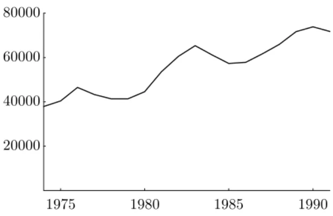
Cycles can be found in Germany, for example, which is illustrated in …gure 1.
The …rst model explaining this phenomenon was proposed by Richard Free- man (1971, 1972, 1975a, 1975b, 1976a, 1976b). His model is based on the assump- tions of myopic wage expectations and occupational immobility.
1We illustrate the model taking the engineering profession as an example. Assume that in an initial period there is an excess demand for engineers. It cannot be satis…ed by physicists, mathematicians, or other college graduates who are occupationally im- mobile. As a consequence, the wage for engineers is high in this period. Because high school graduates are myopic, they believe it will stay high forever. Thus a large number of them enrolls in engineering schools, entering the marketplace in the next period. The excess demand then changes into an excess supply. It can- not be removed by the switching of engineers into other professions. Therefore the wage for engineers is low in this period. Because myopic high school gradu- ates expect it to stay low forever, only few of them enroll in engineering schools this time. The following period is therefore characterized by an excess demand again. Then the process repeats, generating a cobweb pattern of engineering employment.
Freeman’s model is not undisputed. One of the controversial points is whether wage expectations are really myopic. Some evidence supports this hypothesis.
Le-er and Lindsay (1979), for example, …nd that students in medicine base their wage forecasts on current wages. Leonard (1982) shows that personnel executives even in large …rms tend to badly forecast future salaries. Other evidence rejects the hypothesis of myopic wage expectations, supporting the hypothesis of rational wage expectations instead. Willis and Rosen (1979) show that high school gradu- ates can correctly compare future lifetime earnings associated with a high school diploma and future lifetime earnings associated with a college diploma. Ho¤- man and Low (1983) …nd that students in economics can forecast future earnings opportunities very well. Garen (1984) presents evidence implying that young males can correctly forecast lifetime earnings associated with di¤erent levels of schooling. Siow (1984) shows that law students are good predictors of lifetime
1In a more sophisticated version of Freeman’s model, wage expectations are adaptive. This does not make a big di¤erence, however.
1
1975 1980 1985 1990 20000
40000 60000 80000
Figure 1: First-Year Students in Engineering, West Germany, 1974 to 1991 Source: Federal Statistical O¢ce, Statistical Yearbook of the Federal Republic of Germany
earnings. Berger (1988) presents similar …ndings for college majors in general.
Orazem and Mattila (1991), …nally, show that high school graduates are not only able to predict the …rst moment of the future earnings distribution, but also the second one. So several (though not all) studies suggest that wage expectations are rational and not myopic.
2In response to this evidence, Gary Zarkin (1982, 1983, 1985) developed an- other model aimed at explaining cycles in occupational choice. In his model the assumption of myopic wage expectations is replaced by that of rational wage ex- pectations so that occupations are ranked by future expected lifetime earnings and not by current periodical earnings. The assumption of occupational immo- bility is not replaced in the model. For an intuitive understanding, return to the example of the engineering profession. Assume that in an initial period the stock of engineers is low and that it cannot be increased by physicists or other professionals switching into the market for engineers. High school graduates then expect to receive lifetime earnings relatively high when entering the engineering profession. So many of them enroll in engineering schools. As a consequence, the number of new engineers is high in the subsequent period, possibly even higher than the number of old engineers retiring from working life. Since it is not pos- sible for new engineers to switch into another occupation, the stock of engineers increases in this case. High school graduates therefore expect to receive lifetime earnings relatively low when entering the engineering profession. Therefore, rela- tively few of them enroll in engineering schools during this phase. In the following period the number of new engineers thus is low, possibly not even high enough to replace retirees. So the stock of engineers decreases, and expected lifetime
2There is also a study rejecting both the hypothesis of myopic and the hypothesis of rational wage expectations. Betts (1996) …nds that only a minority of students is able to accurately rank four di¤erent occupations by starting salary.
2
earnings rise again. At this point the process repeats, generating equilibrium cycles in the market for new engineers.
3There is some criticism to Zarkin’s model too. The critique refers to the empirical relevance of the assumption of occupational immobility. Many studies
…nd that the degree of occupational mobility is quite high. Börsch-Supan (1990), for example, presents evidence implying that 67 percent of all household heads leave a one digit occupation once or more in 15 years.
4Velling and Bender (1994) show that 13 percent of all employees leave a two digit occupation once a year.
Harper (1995) reports that 11 percent of males in the labor force leave a three digit occupation once a year and that 7 percent do so voluntarily. Mertens (1997) …nds occupational turnover rates of 7 percent a year where occupations are de…ned on the one digit level. Dolton and Kidd (1998), …nally, present evidence implying that 24 percent of male college graduates leave a three digit occupation within the …rst eight years of their working life. This suggests that the assumption of occupational immobility is not consistent with the evidence.
In this paper we present a model which takes this critique seriously. Our model avoids the assumptions of myopic wage expectations and occupational immobility and replaces them by the assumptions of rational wage expectations and perfect occupational mobility. We show that even a model based on these assumptions is able to explain the cyclical behavior of occupational choice observed in many professional labor markets. To simplify the presentation, we proceed in two steps:
In the …rst step, which is found in section 2, we only replace the assumption of myopic wage expectations. In the second step, which is found in section 3, we also abandon the assumption of occupational immobility.
2 A Model with Rational Wage Expectations and Occupational Immobility
Our model is a simple overlapping generations model. In each period a new generation of individuals is born. All generations are equal in size. The size of each generation is normalized to one. Individuals live for two periods. In the
…rst period of life they choose one out of two occupations. In the second period of life they are occupationally immobile and stick to the occupation chosen when young.
5Occupational choice is made in such a way that lifetime earnings are
3Sometimes the model developed by Zarkin is mentioned in one breath with a model de- veloped by Siow (1984). However, Siow’s model can only generate random ‡uctuations in occupational choice. Cycles cannot be generated by the model.
4Studies de…ning occupations on a one/two/three digit level can distinguish up to ten/hundred/thousand di¤erent occupational categories.
5We ignore an extra period when individuals attend college. Such a period could easily be introduced into the model, but it would merely increase complexity without yielding any additional insights.
3
maximized.
6Individuals are hired by …rms. In each period …rms thus employ two generations of individuals in two types of occupations. They use the resulting four types of labor to produce a single good. Production is organized so that pro…ts are maximized.
To …nd the competitive equilibrium of the model, we can either examine the decentralized version of the economy, which is rather tedious and relegated to appendix A, or we can examine the centralized version of the economy, which is much simpler and the way chosen here. The central planner organizes production e¢ciently. He thus maximizes the present value of production
X
1 t=1½
t¡1F ¡
N
tA; N
tAA; N
tB; N
tBB¢
(1) subject to the complementary constraint, the immobility constraints, and the initial condition
N
tB= 1 ¡ N
tA; (2a)
N
tAA= N
tA¡1; (2b)
N
tBB= N
tB¡1; (2c)
N
0A= given (2d)
where t 2 f 0; 1; 2; ::: g is time, ½ 2 (0; 1) is an exogenous discount factor, F 2 [0; 1 ) is a well-behaved production function, N
tA2 [0; 1] is the number of young individuals working in occupation A, N
tAA2 [0; 1] is the corresponding number of old individuals, N
tB2 [0; 1] is the number of young individuals working in occupation B, and N
tBB2 [0; 1] is the corresponding number of old individuals.
7The complementary constraint says that individuals who do not enter A will enter B. The immobility constraints say that old individuals stick to the occupation chosen when young. The initial condition says that the occupational allocation from period zero is predetermined by the time of period one (the planning period).
To …nd the solution of the maximization problem, we insert the constraints from (2a), (2b), and (2c) in the objective function from (1). So we get
X
1 t=1½
t¡1F ¡
N
tA; N
t¡1A; 1 ¡ N
tA; 1 ¡ N
t¡1A¢
: (3)
6Alternatively we could assume occupational choice to be made such that lifetime utility is maximized. However, in this case individuals might react hesitantly to imbalances in lifetime earnings. In a model with perfect occupational mobility the assumption of maximizing lifetime utility is therefore not appropriate.
7For a better understanding of our notation, note that in the next section we will introduce the variablesNtAB andNtBA. They denote the number of individuals changing the occupation when they enter their second period of life.
4
The necessary condition for an inner maximum then is
F
1(X
t) + ½F
2(X
t+1) = F
3(X
t) + ½F
4(X
t+1) (4) with
X
t´ ¡
N
tA; N
t¡1A; 1 ¡ N
tA; 1 ¡ N
t¡1A¢
(5) for t 2 f 1; 2; 3; ::: g . It says that lifetime marginal productivities and, hence, lifetime earnings must equalize across occupations.
The condition of equal lifetime earnings given in (4) determines the dynamics of N
tA. Since we are only interested in linear dynamics,
8we compute the …rst- order Taylor approximation of the necessary condition around the steady state.
As a result we get the linear second-order di¤erence equation G
1¡ N
t+1A¡ N
A¢ + G
2¡ N
tA¡ N
A¢ + G
3¡ N
tA¡1¡ N
A¢
= 0 (6)
where
G
1´ ½F
21¡ ½F
23¡ ½F
41+ ½F
43; (7a) G
2´ F
11¡ F
13¡ F
31+ F
33+ ½F
22¡ ½F
24¡ ½F
42+ ½F
44; (7b)
G
3´ F
12¡ F
14¡ F
32+ F
34(7c)
and where the second partial derivatives of F are evaluated at the steady state.
Note that the shorthand variables G
1, G
2, and G
3may have any numerical value.
The only thing we can say about them is that G
1= ½G
3.
Because we do not know the numerical value of G
1, we must distinguish between two cases. Let us …rst turn to the case where G
1= 0. As G
1= ½G
3, we also have G
3= 0 in this case. So the di¤erence equation from (6) reduces to N
tA= N
A. We see that the number of young individuals entering A is on the steady state level in each period. The number is stationary, cycles in occupational choice do not arise. The model cannot explain the evidence in this case. For this reason we ignore the case from now on.
We now turn to the case where G
16 = 0. In this case it is possible to rewrite the di¤erence equation from (6) as
¡ N
t+1A¡ N
A¢ + H
1¡ N
tA¡ N
A¢ + H
2¡ N
tA¡1¡ N
A¢
= 0 (8)
where
H
1´ G
2G
1= F
11¡ F
13¡ F
31+ F
33+ ½F
22¡ ½F
24¡ ½F
42+ ½F
44½F
21¡ ½F
23¡ ½F
41+ ½F
43; (9a) H
2´ G
3G
1= F
12¡ F
14¡ F
32+ F
34½F
21¡ ½F
23¡ ½F
41+ ½F
43= 1
½ > 1 (9b)
8We ignore the case of nonlinear dynamics because the empirical …ndings of Freeman and Leonard (1978) imply that the economy converges to the steady state. In the neighborhood of the steady state it is su¢cient to study linear dynamics.
5
R
1R
2sign abs sign abs H
12 ( ¡1 ; ¡ 1 ¡ H
2) distinct real roots > 0 < 1 > 0 > 1 H
1= ¡ 1 ¡ H
2distinct real roots > 0 = 1 > 0 > 1 H
12 ¡
¡ 1 ¡ H
2; ¡ 2 p H
2¢ distinct real roots > 0 > 1 > 0 > 1 H
1= ¡ 2 p
H
2identical real roots > 0 > 1 > 0 > 1 H
12 ¡
¡ 2 p
H
2; 2 p H
2¢
conjugate complex roots > 1 > 1 H
1= 2 p
H
2identical real roots < 0 > 1 < 0 > 1 H
12 ¡
2 p
H
2; 1 + H
2¢ distinct real roots < 0 > 1 < 0 > 1 H
1= 1 + H
2distinct real roots < 0 > 1 < 0 = 1 H
12 (1 + H
2; 1 ) distinct real roots < 0 > 1 < 0 < 1 Table 1: The Sign and the Absolute Value of the Characteristic Roots as a Function of the Unknown H
1are two additional shorthand variables. Because we do not know the numerical value of G
1and G
2, we do not know the value of H
1. We know the value of H
2, however, which is equal to 1=½ > 1.
We can solve the di¤erence equation from (8) with standard methods. The general solution of the di¤erence equation is
N
tA¡ N
A=
½ C
1R
t1+ C
2R
t2if H
16 = ¡ 2 p H
2; C
1R
t1+ C
2R
t2t if H
1= ¡ 2 p
H
2(10)
where C
1and C
2are arbitrary constants and R
1and R
2are the characteristic roots
R
1= ¡ H
12 ¡
sµ H
12
¶
2¡ H
2; (11a)
R
2= ¡ H
12 +
sµ H
12
¶
2¡ H
2: (11b)
We analyze the roots in appendix B. The results of the analysis are listed in table 1. As the table shows, the sign and the absolute value of the roots depend on the numerical value of the unknown H
1.
To derive the de…nite solution of the di¤erence equation, we need two bound- ary conditions. One is given by the initial condition
N
0A= given; (12)
which is already known from (2d). The other one is assumed to be
t
lim
!1N
tA= N
A; (13)
6
time entrants
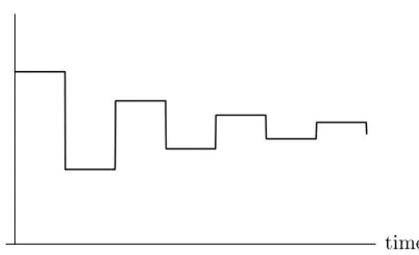
Figure 2: The Time Path of the Number of Young Individuals Entering Occupa- tion A if H
12 (1 + H
2; 1 )
which says that agents expect the economy to converge to the steady state. We could have modelled expectations in any other way, but this way is the only one consistent with the fact that cycles in occupational choice are dampened over time.
As shown in table 1, the economy cannot converge to the steady state if H
12 [ ¡ 1 ¡ H
2; 1 + H
2].
9In this case both roots are equal to or larger than one in absolute value so that convergence is impossible. A de…nite solution satisfying the boundary conditions in (12) and (13) does not exist in this case. If H
12 = [ ¡ 1 ¡ H
2; 1 + H
2], one root is smaller than one in absolute value, however, and convergence is possible. If H
12 ( ¡1 ; ¡ 1 ¡ H
2), the converging root is positive so that the resulting time path of N
tAis monotonic. If H
12 (1 + H
2; 1 ), the converging root is negative so that the time path is oscillatory. The de…nite solution then is
N
tA¡ N
A= ¡
N
0A¡ N
A¢
R
t2: (14)
In this case the model generates cycles in occupational choice which are similar to those we can observe in reality. The number of individuals entering A is cyclical, and cycles are dampened over time. An example for this type of dynamic behavior is given in …gure 2.
What does the condition H
12 (1 + H
2; 1 ) mean? As the de…nitions of H
1and H
2in (9) show, it basically is a technological condition. Given the discount factor ½, it restricts the set of production functions compatible with dampened cycles in occupational choice. A realistic family of production functions satisfying the condition is de…ned by the following three properties:
109This statement is perfectly true only for the linear model. In the nonlinear model conver- gence is impossible ifH1 2(¡1¡H2;1 +H2). The reason for this deviation is that the two versions of the model need not be topologically equivalent atH12 f¡1¡H2;1 +H2g.
10In the following de…nition we use the term substitutes in the sense of Edgeworth or Auspitz-
7
1. Workers who belong to the same occupational group are substitutes, im- plying that F
11< 0, F
12< 0, F
21< 0, F
22< 0, F
33< 0, F
34< 0, F
43< 0, F
44< 0.
2. Workers who belong to di¤erent occupational groups are complements, im- plying that F
13> 0, F
14> 0, F
23> 0, F
24> 0, F
31> 0, F
32> 0, F
41> 0, F
42> 0.
3. Workers who belong to the same occupational and generational group are own-substitutes su¢ciently close, implying that F
11¿ 0, F
22¿ 0, F
33¿ 0, F
44¿ 0.
It is easy to see from (9) that for production functions from this family the condition H
12 (1 + H
2; 1 ) is satis…ed.
If we stay with this type of production function for another moment, we can easily explain the intuition of our model. Assume that in an initial period there are many old workers in A and few old workers in B. Because young workers in A are substitutes for old workers in A and complements to old workers in B , this implies that young workers who enter A receive low lifetime earnings. Because young workers in B are complements to old workers in A and substitutes for old workers in B, this also implies that young workers who enter B receive high lifetime earnings. So only few young workers enter A and many young workers enter B. In the next period the number of old workers in A thus is low and the number of old workers in B is high. The scheme of substitutability and complementarity then implies that young workers receive high lifetime earnings when entering A and low lifetime earnings when entering B. So many young workers choose A and few young workers choose B. The following period thus is characterized by a high number of old workers in A and a low number of old workers in B again. At this point the process repeats, generating cycles in occupational choice.
3 A Model with Rational Wage Expectations and Perfect Occupational Mobility
Critical to the model presented in the last section is the assumption that old indi- viduals are occupationally immobile. Now we abandon this assumption and allow for perfect occupational mobility. In each period we thus have young individuals entering A or B (called entrants), old individuals staying in A or B (called stay- ers), and old individuals switching from A to B or from B to A (called switchers).
Firms employ these six types of workers. What is the competitive equilibrium?
Lieben substitutes. Similarly, we use the term complements in the sense of Edgeworth or Auspitz-Lieben complements.
8
Again the competitive equilibrium can easier be found by employing the con- cept of the central planner (for the decentralized version of the economy see appendix A). The central planner maximizes
X
1 t=1½
t¡1F ¡
N
tA; N
tAA; N
tB; N
tBB; N
tAB; N
tBA¢
(15) subject to the constraints
N
tB= 1 ¡ N
tA; (16a)
N
tAA= N
tA¡1¡ N
tAB; (16b) N
tBB= N
tB¡1¡ N
tBA; (16c)
N
0A= given (16d)
where N
tAB2 £
0; N
tA¡1¤
and N
tBA2 £
0; N
tB¡1¤
are the numbers of old individuals switching from A to B and from B to A. Note that the production function has six arguments now [compare (15) to (1)]. Note also that we have two switching constraints instead of two immobility constraints [compare (16b) and (16c) to (2b) and (2c)]. The switching constraints say that the number of stayers by de…nition is equal to the number of former entrants minus the number of switchers.
To solve the maximization problem, we insert the constraints from (16a), (16b), and (16c) into the objective function from (15):
X
1 t=1½
t¡1F ¡
N
tA; N
tA¡1¡ N
tAB; 1 ¡ N
tA; 1 ¡ N
tA¡1¡ N
tBA; N
tAB; N
tBA¢
: (17) The necessary conditions for an inner maximum then are
F
1(X
t) + ½F
2(X
t+1) = F
3(X
t) + ½F
4(X
t+1) ; (18a)
F
2(X
t) = F
5(X
t) ; (18b)
F
4(X
t) = F
6(X
t) (18c)
with
X
t´ ¡
N
tA; N
tA¡1¡ N
tAB; 1 ¡ N
tA; 1 ¡ N
tA¡1¡ N
tBA; N
tAB; N
tBA¢
(19) for t 2 f 1; 2; 3; ::: g . They imply that lifetime earnings must equalize across occu- pations, and that periodical earnings must equalize across stayers and switchers.
The necessary conditions determine the dynamics of N
tA, N
tAB, and N
tBA. Restricting ourselves again to the linear dynamic case, we compute the …rst- order Taylor approximation of the necessary conditions around the steady state.
9
This leads to the system of linear second-order di¤erence equations
0
@ G
11G
12G
13G
14G
15G
16G
170 0 0 G
24G
25G
26G
270 0 0 G
34G
35G
36G
371 A
0 B B B B B B B B
@
N
t+1A¡ N
AN
t+1AB¡ N
ABN
t+1BA¡ N
BAN
tA¡ N
AN
tAB¡ N
ABN
tBA¡ N
BAN
tA¡1¡ N
A1 C C C C C C C C A
= 0
@ 0 0 0
1 A (20)
where
G
11´ ½F
21¡ ½F
23¡ ½F
41+ ½F
43; (21a)
G
12´ ¡ ½F
22+ ½F
25+ ½F
42¡ ½F
45; (21b) G
13´ ¡ ½F
24+ ½F
26+ ½F
44¡ ½F
46; (21c) G
14´ F
11¡ F
13+ ½F
22¡ ½F
24¡ F
31+ F
33¡ ½F
42+ ½F
44; (21d)
G
15´ ¡ F
12+ F
15+ F
32¡ F
35; (21e)
G
16´ ¡ F
14+ F
16+ F
34¡ F
36; (21f)
G
17´ F
12¡ F
14¡ F
32+ F
34; (21g)
G
24´ F
21¡ F
23¡ F
51+ F
53; (21h)
G
25´ ¡ F
22+ F
25+ F
52¡ F
55; (21i)
G
26´ ¡ F
24+ F
26+ F
54¡ F
56; (21j)
G
27´ F
22¡ F
24¡ F
52+ F
54; (21k)
G
34´ F
41¡ F
43¡ F
61+ F
63; (21l)
G
35´ ¡ F
42+ F
45+ F
62¡ F
65; (21m)
G
36´ ¡ F
44+ F
46+ F
64¡ F
66; (21n)
G
37´ F
42¡ F
44¡ F
62+ F
64: (21o)
Note that some G
ij’s are related to each other:
G
11= ½G
17; (22a)
G
12= ¡ ½G
27; (22b)
G
13= ¡ ½G
37; (22c)
G
15= ¡ G
24; (22d)
G
16= ¡ G
34; (22e)
G
26= G
35: (22f)
More information about these variables is not available. In particular, we cannot tell anything about their numerical value.
We now use the system of di¤erence equations to derive a single di¤erence equation that governs the dynamics of N
tA. For this purpose we rewrite the
10
system, taking into account that the last two equations, which refer to t and t ¡ 1, also refer to t + 1 and t:
0 B B B B
@
G
11G
12G
13G
14G
15G
16G
170 0 0 G
24G
25G
26G
270 0 0 G
34G
35G
36G
37G
24G
25G
26G
270 0 0 G
34G
35G
36G
370 0 0
1 C C C C A
0 B B B B B B B B
@
N
t+1A¡ N
AN
t+1AB¡ N
ABN
t+1BA¡ N
BAN
tA¡ N
AN
tAB¡ N
ABN
tBA¡ N
BAN
tA¡1¡ N
A1 C C C C C C C C A
= 0 B B B B
@ 0 0 0 0 0
1 C C C C
A : (23)
Then we rearrange the system as follows:
0 B B B B
@
G
11G
12G
13G
15G
160 0 0 G
25G
260 0 0 G
35G
36G
24G
25G
260 0 G
34G
35G
360 0
1 C C C C A
0 B B B B
@
N
t+1A¡ N
AN
t+1AB¡ N
ABN
t+1BA¡ N
BAN
tAB¡ N
ABN
tBA¡ N
BA1 C C C C A =
¡ 0 B B B B
@
G
14G
17G
24G
27G
34G
37G
270 G
370
1 C C C C A
µ N
tA¡ N
AN
t¡1A¡ N
A¶
: (24)
Now we apply Cramer’s rule to solve the system for N
t+1A¡ N
A.
11So we get N
t+1A¡ N
A= ¡ H
11¡
N
tA¡ N
A¢
¡ H
12¡
N
tA¡1¡ N
A¢
(25) with
H
11´
¯ ¯
¯ ¯
¯ ¯
¯ ¯
¯ ¯
G
14G
12G
13G
15G
16G
240 0 G
25G
26G
340 0 G
35G
36G
27G
25G
260 0 G
37G
35G
360 0
¯ ¯
¯ ¯
¯ ¯
¯ ¯
¯ ¯
¯ ¯
¯ ¯
¯ ¯
¯ ¯
¯ ¯
G
11G
12G
13G
15G
160 0 0 G
25G
260 0 0 G
35G
36G
24G
25G
260 0 G
34G
35G
360 0
¯ ¯
¯ ¯
¯ ¯
¯ ¯
¯ ¯
; (26a)
11We assume that the determinant of the coe¢cient matrix on the left of (24) is di¤erent from zero. This way we exclude special cases similar to that we encountered in the last section.
There occupational choice was stationary ifG1= 0.
11
H
12´
¯ ¯
¯ ¯
¯ ¯
¯ ¯
¯ ¯
G
17G
12G
13G
15G
16G
270 0 G
25G
26G
370 0 G
35G
360 G
25G
260 0 0 G
35G
360 0
¯ ¯
¯ ¯
¯ ¯
¯ ¯
¯ ¯
¯ ¯
¯ ¯
¯ ¯
¯ ¯
¯ ¯
G
11G
12G
13G
15G
160 0 0 G
25G
260 0 0 G
35G
36G
24G
25G
260 0 G
34G
35G
360 0
¯ ¯
¯ ¯
¯ ¯
¯ ¯
¯ ¯
: (26b)
Equation (25) is the di¤erence equation we have looked for. Note that it is free from the switching variables N
tABand N
tBA. Although we allow for occupational switches in this model, the corresponding variables do not appear in the di¤erence equation governing the dynamics of N
tA. As a result, the di¤erence equation we get in this section is very similar to that obtained in the last section [compare (25) to (8)]. The two di¤erence equations have the same structure, and they share an identical coe¢cient. By inserting (22) into (26b) and expanding determinants, we can see that H
12is equal to 1=½ and, thus, to H
2. Any di¤erence between the model with and the model without occupational mobility thus is re‡ected in the di¤erence between H
11and H
1.
Since the two di¤erence equations are nearly identical, we can solve them in the same way. By following the procedure described in the last section, we
…nd that the time path of N
tAexhibits dampened cycles if the condition H
112 (1 + H
12; 1 ) is satis…ed. This condition again has a technological character. It restricts the set of production functions compatible with dampened cycles in occupational choice. Let us examine if the family of production functions de…ned by the following three properties satis…es the condition:
1. Workers who currently belong to the same occupational group are substi- tutes, implying that F
11< 0, F
12< 0, F
16< 0, F
21< 0, F
22< 0, F
26< 0, F
33< 0, F
34< 0, F
35< 0, F
43< 0, F
44< 0, F
45< 0, F
53< 0, F
54< 0, F
55< 0, F
61< 0, F
62< 0, F
66< 0.
2. Workers who currently belong to di¤erent occupational groups are comple- ments, implying that F
13> 0, F
14> 0, F
15> 0, F
23> 0, F
24> 0, F
25> 0, F
31> 0, F
32> 0, F
36> 0, F
41> 0, F
42> 0, F
46> 0, F
51> 0, F
52> 0, F
56> 0, F
63> 0, F
64> 0, F
65> 0.
3. Workers who belong to the same occupational, generational, and transi- tional group are own-substitutes su¢ciently close, implying that F
11¿ 0, F
22¿ 0, F
33¿ 0, F
44¿ 0, F
55¿ 0, F
66¿ 0.
12
In the previous section it was easy to see that the example family of production functions satis…es the condition for dampened cycles in occupational choice. This time it is rather di¢cult to see this although the families are very similar in both sections. Therefore we approached the problem numerically. We assigned numerical values to F
11; F
12; ::: that conformed to the pattern de…ned by the three properties. We also assigned a value to ½. Then we computed H
11and H
12and checked if the cycle condition was satis…ed. We found that for some parameterizations it was, while for others it was not.
12So the family of production functions de…ned above does not satisfy the cycle condition in any case. In many cases the condition is met, however. Cycles in occupational choice therefore are possible even if occupational mobility is perfect among workers.
4 Conclusion
Many professional labor markets exhibit systematic ups and downs. There are periods when many new workers enter these markets, followed by periods when there are only few entrants. This phenomenon can be observed on the markets for engineers, physicists, mathematicians, and others. Richard Freeman (1971, 1972, 1975a, 1975b, 1976a, 1976b) has proposed to explain the phenomenon by means of a cobweb model based on the assumptions of myopic wage expecta- tions and occupational immobility. However, some evidence suggests that wage expectations are rational and not myopic. Students in economics and law, for example, have been shown to form their wage expectations rationally. In re- sponse to this evidence, Gary Zarkin (1982, 1983, 1985) has proposed to explain the phenomenon by means of a rational expectations model based only on the assumption of occupational immobility. Nevertheless, there is reason to question this assumption as well. Empirical studies report occupational turnover rates between seven and thirteen percent a year. In the long run, about two thirds of all workers seem to change their occupation even if occupations are de…ned very broadly. Taking this evidence seriously, we have presented a model in this paper which is neither based on the assumption of myopic wage expectations nor on that of occupational immobility. It is based instead on the assumptions of rational wage expectations and perfect occupational mobility. We have shown that even a model based on these assumptions can explain the existence of cycles in occupational choice. There are plausible technologies for which cycles do not
12We selected the numbers for Fij randomly. If Fij < 0 and i 6= j, the numbers were uniformly drawn from the interval [¡1;0]. If Fij <0and i = j, they were uniformly drawn from[¡7:5;¡5]. IfFij >0, they were uniformly drawn from [0;1]. The number assigned to½ was0:5. We performed100 experiments. The condition for converging cycles was satis…ed in 53cases, in47 cases it was not. When the model generated cycles, they were weaker than in the model with occupational immobility. When it did not generate cycles, the time path was nevertheless converging. Since the model is quite abstract, one should not overemphasize the numerical results.