An enhanced model for portfolio choice with SSD criteria: a constructive approach
Csaba I. F´abi´an
∗Gautam Mitra
†Diana Roman
‡Victor Zverovich
§∗Institute of Informatics, Kecskem´et College, 10 Izs´aki ´ut, 6000 Kecskem´et, Hungary; and Dept of OR, Lor´and E¨otv¨os Univ.
E-mail: fabian.csaba@gamf.kefo.hu.
†CARISMA: The Centre for the Analysis of Risk and Optimisation Modelling Applications, School of Information Systems, Computing and Mathematics, Brunel University, UK. E-mail: gautam.mitra@brunel.ac.uk
‡CARISMA: The Centre for the Analysis of Risk and Optimisation Modelling Applications, School of Information Systems, Computing and Mathematics, Brunel University, UK. E-mail: diana.roman@brunel.ac.uk
§CARISMA: The Centre for the Analysis of Risk and Optimisation Modelling Applications, School of Information Systems, Computing and Mathematics, Brunel University, UK. E-mail: viktar.zviarovich@brunel.ac.uk
1 Abstract
We formulate a portfolio planning model which is based on Second-order Stochastic Dominance as the choice criterion. This model is an enhanced version of the multi-objective model proposed by Roman, Darby- Dowman, and Mitra (2006); the model compares the scaled values of the different objectives, representing tails at different confidence levels of the resulting distribution. The proposed model can be formulated as risk minimisation model where the objective function is a convex risk measure; we characterise this risk measure and the resulting optimisation problem. Moreover, our formulation offers a natural generalisation of the SSD-constrained model of Dentcheva and Ruszczy´nski (2006). A cutting plane-based solution method for the proposed model is outlined. We present a computational study showing: (a) the effectiveness of the solution methods and (b) the improved modelling capabilities: the resulting portfolios have superior return distributions.
2 Introduction
2.1 Second-order Stochastic Dominance
LetRandR0 denote random returns. Second-order Stochastic Dominance (SSD) is defined by the following equivalent conditions:
(a) E (U(R))≥E (U(R0)) holds for any increasing and concave (integrable) utility function U.
(b) E ([t−R]+) ≤ E ([t−R0]+) holds for eacht∈IR.
(c) Tailα(R) ≥ Tailα(R0) holds for each 0< α≤1, where Tailα(R) denotes the unconditional expectation of the leastα∗100% of the outcomes ofR.
For the equivalence of (a)and (b) see for example Whitmore and Findlay (1978). The equivalence of (b) and (c) is shown in Ogryczak and Ruszczy´nski (2002): they consider Tailα(R) as a function of α, and E ([t−R]+) as a function oft; and observe that these functions are convex conjugates.
If(a b c)above hold, we say thatRdominatesR0 with respect to SSD, and use the notationRºSSD R0. The corresponding strict dominance relation is defined in the usual way: RÂSSD R0 means thatRºSSDR0 andR06ºSSD R.
In this paper we deal with portfolio returns. Letndenote the number of the assets into which we may invest at the beginning of a fixed time period. A portfoliox= (x1, . . . xn)∈IRn represents the proportions of the portfolio value invested in the different assets. Let the n-dimensional random vectorR denote the returns of the different assets at the end of the investment period. It is usual to consider the distribution of R as discrete, described by the realisations under various scenarios. The random return of portfolio x will be Rx:=x1R1+. . . xnRn.
LetX ⊂IRndenote the set of the feasible portfolios. We assume thatXis a bounded convex polyhedron.
A portfoliox? is said to be SSD-efficient if there is no feasible portfoliox∈X such thatRxÂSSD Rx?. The importance of SSD as a choice criterion in portfolio selection, as well as the difficulty in applying it in practice have been widely recognised (Hadar and Russell 1969, Whitmore and Findlay 1978, Kroll and Levy 1980, Ogryczak and Ruszczynski 2001, 2002). SSD is a meaningful choice criterion, due to its relation to risk averse behaviour (as stated at (a)), which is the general assumption about investment behaviour. The computational difficulty of the SSD-based models arises from the fact that, finding the set of SSD efficient portfolios is a model with a continuum of objectives (as stated at (c)). Only recently, SSD-based portfolio models based have been proposed (Dentcheva and Ruszczynski 2003, 2006, Roman et al. 2006, Fabian et al.
2008).
2.2 Portfolio models based on the SSD criteria
The SSD-based models reviewed here assume that a reference random return R, with a known (discrete)b distribution, is available;Rb could be for example the return of a stock index or of a benchmark portfolio.
Dentcheva and Ruszczy´nski (2006) propose an SSD constrained portfolio optimisation model:
max f(x) such that x∈X,
RxºSSD R,b
(1)
where f is a concave function. In particular, they consider f(x) = E (Rx). They formulate the problem using criterion(b)(section 2.1) and prove that, in case of finite discrete distributions, the SSD relation can be characterised by a finite system of inequalities from those in(b). The authors developed a solution method based on a dual formulation and the Regularized Decomposition method of Ruszczynski (1986). The authors implemented this method, using a dataset with with 719 real-world assets and 616 possible realizations of their joint return rates; favorable performance is reported.
Roman, Darby-Dowman, and Mitra (2006) use criterion(c)(section 2.1). They assume finite discrete dis- tributions with equally probable outcomes, and prove that, in this case, the SSD relation can be characterised by a finite system of inequalities. Namely, Rx ºSSD Rb is equivalent to Taili
S
¡Rx¢
≥ Taili
S
¡Rb¢ (i = 1, . . . , S), where S is the number of (equally probable) scenarios. The authors propose a multi-objective model whose Pareto optimal solutions are SSD-efficient portfolios.
A specific solution is chosen whose return distribution comes close to, or emulates, the reference return Rb in a uniform sense. Uniformity is meant in terms of differences among tails; the ”worst” tail difference ϑ= min
i=1...S
¡Taili
S
¡Rx¢
−Taili
S
¡Rb¢¢
is maximised:
max ϑ
such that ϑ∈IR, x∈X, Taili
S
¡Rx¢
≥ Taili
S
¡Rb¢
+ϑ (i= 1, . . . , S).
(2)
The return distribution of the chosen portfolio comes ”close or better” than the reference distribution:
if the reference distribution is not SSD efficient (which is often the case), the model improves on it until SSD-efficiency is reached.
The authors implemented the model outlined above, and made extensive testing on problems with 76 real- world assets using 132 possible realisations of their joint return rates. Powerful modelling capabilities were demonstrated by in-sample and out-of-sample analysis of the return distributions of the optimal portfolios.
2.3 An enhanced model
In this paper we propose a scaled version of the model (2) of Roman, Darby-Dowman, and Mitra (2006).
The new model is formulated in the compact form max ϑ
such that ϑ∈IR, x∈X, Rx ºSSDRb+ϑ.
(3)
Obviously we have Taili
S
¡Rb+ϑ¢
= Taili
S
¡Rb¢
+Si ϑ (i= 1, . . . , S) withϑ∈IR. Hence, using criterion (c) (section 2.1), the model (3) can be equivalently formulated as
max ϑ
such that ϑ∈IR, x∈X, Taili
S
¡Rx¢
≥ Taili S
¡Rb¢
+Si ϑ (i= 1, . . . , S).
(4)
The difference between (2) and (4) is that the tails are scaled in the latter model.
This approach has several advantages; one of them lies in the connection with the risk minimisation theory.
The quantityϑin (4) measures the preferability of the portfolio returnRxrelative to the reference return R.b
The relationRxºSSD R+ϑb means that we prefer the return distribution of portfolioxto the combination of the reference return and a certain returnϑ(usually cash).
We can introduce an opposite measure as b
ρ¡ R¢
:= min n
%∈IR
¯¯
¯R+%ºSSD Rb o
for any returnR. (5)
In words,ρb¡ R¢
measures the amount of certain return whose addition makesRpreferable toR.b Using this, the problem (3) can be formulated as
xmin∈X ρb¡ Rx¢
. (6)
We show thatρbis aconvex risk measure. We also develop a cutting-plane representation of bρby adapting the approach presented in F´abi´an, Mitra, and Roman (2008). This gives a solution method for problem (6).
Using the risk measureρ, an extension of the SSD-constrained model (1) of Dentcheva and Ruszczy´b nski can be formulated as
max f(x) such that x∈X,
b ρ¡
Rx¢
≤γ,
(7)
whereγ ∈IR is a parameter. In an application, the setting of the parameter γis usually the responsibility of the decision makers. We can help them by constructing the efficient frontier. Suppose that values and subgradients can be computed to the functionf. The efficient frontier of problem (7) can be approximated by solving Lagrangian problems
maxx∈X f(x)−λρb¡ Rx¢
(8) with different values of λ≥0. Once the right-hand-side parameter γ is tuned by the decision maker, the problem can be solved by a constrained convex method.
The paper is organised as follows:
In Section 3, we overview coherent and convex risk measures, and show thatρbdefined as (5) is a convex risk measure. We also present the dual representation ofρ.b
In Section 4, we compare different formulations of the enhanced portfolio choice problem (3).
In Section 5, we describe a cutting-plane approach for the enhanced portfolio choice problem (3), and study its convergence. We also sketch a solution method for the problem (7).
In Section 6, we present a computational study. We compare the return distributions of the respective optimal portfolios belonging to the multi-objective problem of Roman, Darby-Dowman, and Mitra (2) on the one hand, and to the scaled version (4) on the other hand.
The results are summarised in Section 7.
3 Convex risk measures
3.1 Overview of risk measures
LetR denote a subspace of random returns R: Ω →IR. A risk measure is mapping ρ: R →[−∞,+∞].
Theacceptance setof a risk measure ρis defined as
Aρ:={R∈ R |ρ(R)≤0}. (9) Conversely, anacceptance setAdefines a risk measureρA:
ρA(R) := inf{%∈IR|R+%∈ A } (R∈ R). (10) The concept of coherent risk measureswas developed by Artzner et al. (1999) and Delbaen (2002). These measures satisfy the four criteria of sub-additivity, positive homogeneity, monotonicity, and translation equivariance. The acceptance set of a coherent measure is a convex cone.
A well-known example for a coherent risk measure is Conditional Value-at-Risk(CVaR), charactarised by Rockafellar and Uryasev (2000, 2002). In words, CVaRα(R) is the conditional expectation of the upper α-tail of −R. (In our setting,Rrepresents gain, hence −R represents loss.) We have the relation
CVaRα(R) =−1
αTailα(R) (0< α≤1). (11)
(In Rockafellar and Uryasev (2000, 2002), CVaR is defined with respect to a general loss function.)
The concept ofconvex risk measuresis a natural generalisation of coherency, which allows more general convex sets as acceptance sets. The concept was introduced by Heath (2000), Carr, Geman, and Madan (2001), and F¨ollmer and Schied (2002). A risk measure ρ is said to be convex if it satisfies the following criteria:
Convexity: ρ¡
λR+ (1−λ)R0¢
≤λρ(R) + (1−λ)ρ(R0) holds forR, R0∈ Rand 0≤λ≤1.
Monotonicity: ρ(R)≤ρ(R0) holds forR, R0 ∈ R, R≥R0.
Translation equivariance: ρ(R+%) =ρ(R)−%holds forR∈ R, %∈IR.
Rockafellar, Uryasev, and Zabarankin (2002, 2006) develop another generalisation of the coherency concept, which also includes thescalability criterion: ρ(R%) =−%for each%∈IR (hereR%∈ Rdenotes the return of constant%). An overview can be found in Rockafellar (2007).
The above cited works also develop dual representations of risk measures. A coherent risk measure can be represented as
ρ(R) = sup
Q∈QEQ(−R), (12)
where Qis a set of probability measures on Ω. A risk measure that is convex or coherent in the extended sense of Rockafellar et al., can be represented as
ρ(R) = sup
Q∈Q
n
EQ(−R)− α(Q)o
, (13)
where Q is a set of probability measures, and αis a mapping from the set of the probability measures to (−∞,+∞]. (Properties of Q and α depend on the type of risk measure, and also on space R, and the topology used.) On the basis of these dual representations, an optimisation problem that involves a risk measure can be interpreted as a robust optimisation problem.
Ruszczy´nski and Shapiro (2006) develop optimality and duality theory for problems with convex risk functions.
3.2 Convexity of the risk measure ρ
bThe risk measureρbdefined in (5) derives from the acceptance setAb:=
n R∈ R
¯¯
¯RºSSD Rb o
in the manner of (10). We prove convexity ofρbusing the following proposition from F¨ollmer and Schied (2002):
Proposition 1 Let Abe a convex subset ofR, such that
A 6=∅ and ρA(R0)>−∞, (14) whereR0∈ R denotes the return of constant0. Suppose thatAhas the following property:
if R∈ A and R0∈ R, R0 ≥R, then R0 ∈ A. (15) ThenρA, defined as (10), is a convex risk measure. (If, moreover,Asatisfies a certain closedness criterion, thenA=AρA holds.)
In the remaining part of this subsection, we just show thatAbsatisfies the criteria of Proposition 1.
In order to prove that Abis convex, letR, R0 ∈A, i.e.,b R, R0ºSSDR. We show thatb λR+ (1−λ)R0∈Ab for 0≤λ≤1. Let us first observe that the dominance criterion(a) of Section 2.1 can be reformulated as
(a0) EU(R)≥EU(R0) for any monotonic and concave (integrable) utility functionU havingU(R0) = 0.
LetU be a such a utility function. Expected utility inherits concavity ofU, hence we have EU¡
λR+ (1−λ)R0¢
≥ EU(λR) + EU¡
(1−λ)R0¢
. (16)
The functionλ7→EU(λR) is obviously concave, and forλ= 0 or 1 we have EU(λR) =λEU(R). Hence EU(λR) ≥ λEU(R) and EU¡
(1−λ)R0¢
≥ (1−λ)EU(R0). (17) From our assumptions, we have
EU(R), EU(R0) ≥EU(R).b (18)
Putting (16), (17), (18) together, we get EU¡
λR+ (1−λ)R0¢
≥ EU(R).b
According to(a0) above, this impliesλR+ (1−λ)R0ºSSD R, which proves convexity ofb A.b Abevidently satisfies (14), and (15) is a consequence of the monotonicity of our utility functions.
3.3 Dual representation of ρ
bIn order to construct a dual representation of ρ, we follow the approach of Rockafellar, Uryasev, andb Zabarankin. The space R of returns is L2 = L2(Ω,M, P), i.e., the measurable functions for which the mean and variance exists. (The set Ω is equipped with the probability measure P, the field of measurable sets beingM.) As for probability measures, Rockafellar at al. focus on those that can be described by den- sity functions with respect toP. Moreover the density functions need to fall into L2. LetQbe a legitimate probability measure with density functiondQ. Under these conditions EQ(R) =E(R dQ) holds.
Rockafellar at al. show that the dual representation of CVaRαin the form of (12) is CVaRα(R) = sup
dQ≤α−1
EQ(−R) (0< α≤1). (19)
Based on this result, we construct a dual representation of ρ. According to the definitionb (c) of SSD in Section 2.1, we have
Ab= \
0<α≤1
Bbα (20)
with Bbα:=
n R
¯¯
¯Tailα(R)≥Tailα(R)b o
= n
R
¯¯
¯CVaRα(R)≤CVaRα(R)b o
(0< α≤1).
(The above equality is an obvious consequence of (11).) Substituting (19) we get Bbα=n
R
¯¯
¯EQ(−R)≤CVaRα(R) holds for eachb QhavingdQ ≤α−1o
(0< α≤1).
Substituting this into (20), we get Ab= n
R
¯¯
¯EQ(−R)≤CVaRα(R) holds for each (Q, α) havingb dQ≤α−1o
. (21)
Let us define
Q:={Q|supdQ<+∞ } and s(Q) :=¡ sup dQ
¢−1
(Q∈ Q).
(We haves(Q)≤1 for each legitimateQ.) Equality (21) can be continued as Ab =
n R
¯¯
¯EQ(−R)≤CVaRα(R) holds for eachb Q∈ Q, α≤s(Q) o
= n
R
¯¯
¯EQ(−R)≤CVaRs(Q)(R) holds for eachb Q∈ Q o
, since CVaRα(R) is decreasing function ofb α. We haveρb=ρAb hence by (10)
b
ρ(R) = inf n
%∈IR
¯¯
¯EQ(−R−%)≤CVaRs(Q)(R) holds for eachb Q∈ Qo
= sup
Q∈Q
n
EQ(−R) −CVaRs(Q)(R)b o (22)
holds for eachR∈ R, and this has the form of the dual representation (13) withα(Q) = CVaRs(Q)(R).b In the remaining part of this paper we focus on discrete finite distributions with equiprobable outcomes. In this caseRis a finite dimensional space, and the acceptance setAbis a polyhedron with a highly symmetric structure.
4 Problem formulation
We compare different formulations of the enhanced model (3). The dominance relation can be formulated by either tails or integrated chance constraints, according to criterions(b)or (c)in Section 2.1.
We assume that the joint distribution of R and Rb is discrete finite, having S equally probable out- comes. Let r(1), . . . , r(S) denote the realisations of the random R vector of asset returns. Similarly, let b
r(1), . . . , rb(S) denote realisations of the reference return R. For the reference tails, we will use the briefb notationbτi:= Taili
S
¡Rb¢
(i= 1, . . . S).
4.1 Formulation using tails
In their multi-objective model (2), Roman, Darby-Dowman, and Mitra computed tails in the following form, by adapting the CVaR-optimisation formula of Rockafellar and Uryasev (2000, 2002):
Taili
S
¡Rx¢
= max
ti∈IR
i S ti− 1
S XS
j=1
h
ti−r(j)Tx i
+
.
Roman et al. then formulated (2) in linear programming form, introducing new variables for the positive parts
£ti−r(j)Tx¤
+. The resulting problems were found to be computationally demanding, though. Instead of introducing new variables, F´abi´an, Mitra, and Roman (2008) used the following cutting-plane representation, adapting the approach of K¨unzi-Bay and Mayer (2006):
Taili
S
¡Rx¢
= min S1 P
j∈Ji
r(j)Tx
such that Ji ⊂ {1, . . . , S}, |Ji|=i.
(23)
The above formula enables a cutting-plane approach to the multi-objective model (2). F´abi´an et al. imple- mented this cutting-plane approach, and found it highly effective.
Applying (23) to the present, scaled-tail model (4) results the following cutting-plane representation:
max ϑ
such that ϑ∈IR, x∈X,
i
Sϑ+τbi ≤ S1 P
j∈Ji
r(j)Tx for each Ji⊂ {1, . . . , S}, |Ji|=i, where i= 1, . . . , S.
(24)
4.2 Formulation using integrated chance constraints
In their SSD-constrained model (1), Dentcheva and Ruszczy´nski characterise stochastic dominance with crite- rion(b)in Section 2.1. They prove that ifRbhas a discrete finite distribution with realisationsbr(1), . . . , br(S), thenRxºSSD Rb is equivalent to a finite system of inequalities
E µh
b
r(i)−Rx i
+
¶
≤ E µh
b r(i)−Rb
i
+
¶
(i= 1, . . . , S).
The constraintRxºSSDRb+ϑof the present enhanced model (3) can be formulated in the same manner:
XS
j=1
1 S
h b
r(i)+ϑ−r(j)Tx i
+ ≤
XS
j=1
1 S
h b
r(i)−br(j) i
+ (i= 1, . . . , S). (25) The inequalities in (25) are integrated chance constraints, and can be formulated as finite sets of linear inequalities using the cutting-plane representation of Klein Haneveld and Van der Vlerk (2006). These authors also present a computational study demonstrating the effectiveness of their cutting-plane approach for optimisation problems. The cutting-plane representation of theith constraint from our system (25) is
X
j∈Ji
1 S
n b
r(i)+ϑ−r(j)Txo
≤ XS
j=1
1 S
h b
r(i)−rb(j)i
+ for eachJi⊂ {1, . . . , S}.
Using the above cutting-plane representation for each integrated chance constraint, the enhanced model (3) can be formulated as
max ϑ
such that ϑ∈IR, x∈X, P
j∈Ji
1 S
n b
r(i)+ϑ−r(j)Txo
≤ PS
j=1 1 S
£rb(i)−br(j)¤
+ for eachJi⊂ {1, . . . , S}, wherei= 1, . . . , S.
(26)
The problems (26) and (24) are equivalent since they are different formulations of the enhanced model (3).
To be specific, we can find a mapping between the two constraint sets: For the sake of simplicity, assume that the realisations of the reference return are ordered: br(1)≤. . .≤rb(S). It is easily seen that the constraint belonging to a setJi⊂ {1, . . . , S}in (26) is
– equivalent to the constraint belonging toJi in (24), if|Ji|=i;
– redundant if|Ji| 6=i.
In the remaining part of this paper we will use the formulation (24) as it is more economic under our assumptions.
Remark 2 If we drop the equiprobability assumption, but keep the discrete finite assumption, then the for- mulation (26) will be more convenient.
4.3 Connection with risk measures
Changing the scope of optimisation, problem (24) can be formulated as minimisation of a polyhedral convex function:
xmin∈X ϕ(x) where ϕ(x) := max (
−1i P
j∈Ji
r(j)Tx +Siτbi
)
such that Ji⊂ {1, . . . , S}, |Ji|=i, where i= 1, . . . , S.
(27)
We have Sibτi =−CVaRi
S(R) according to (11). The above definition ofb ϕ is just the specialisation of the dual representation (22) to the present discrete, finite, equiprobable case. Hence we have ϕ(x) = ρb¡
Rx¢ with the convex risk measure introduced in Section 3.
5 Solution methods
We solve the portfolio optimisation problem in the form (27).
5.1 Pure cutting plane method
Applied to a convex programming problem min
x∈X φ(x), the cutting plane method generates a sequence of iterates fromX. At each iterate, supporting linear functions (cuts) are constructed to the objective function.
A cutting-plane model of the objective function is then maintained as the upper cover of known cuts. The next iterate is obtained by minimising the current model function overX.
Cutting plane methods are considered fairly efficient for quite general problem classes. However, according to our knowledge, efficiency estimates only exist for the continuously differentiable, strictly convex case. An overview can be found in Dempster and Merkovsky (1995), who present a geometrically convergent version.
Supporting linear functions to our present objective functionϕin (27) are easily constructed:
– Givenx?∈X, let rx(j1??)≤. . .≤r(jx??S) denote the ordered outcomes ofRx?=RTx?.
– Using this ordering of the scenarios, let us construct the sets Ji?:={j1?, . . . , ji?} (i= 1, . . . , S).
– Let us selecti?∈arg max
1≤i≤S
(
−1i P
j∈Ji?
r(j)Tx? +Siτbi
) .
– A supporting linear function atx?is then l(x) := −i1?
P
j∈Ji??
r(j)Tx +iS?bτi?.
Klein Haneveld and Van der Vlerk (2006), K¨unzi-Bay and Mayer (2006), F´abi´an, Mitra, and Roman (2008) report application of the cutting plane method to stochastic programming problems similar to the present one. The method proved very effective for these problems. When a problem was solved with increasing numbers of scenarios, the iteration count increased very slowly.
5.2 Level method
The level method is a regularised cutting plane method, proposed by Lemar´echal, Nemirovskii, and Nesterov (1995). A cutting-plane model function is maintained as in the pure cutting plane method. The next iterate is obtained by minimising the current model function over the feasible domain, and then projecting the minimiser to a certain level set of the current model function. (Projecting requires the solution of a convex quadratic programming problem.)
Lemar´echal, Nemirovskii, and Nesterov prove the following efficiency estimate: Suppose that the objective function is Lipschitz-continuous with the parameterL, and letDdenote the diameter of the feasible domain.
To obtain an²-optimal solution, it suffices to perform c¡LD
²
¢2
iterations, wherecis a constant. Lemar´echal, Nemirovskii, and Nesterov also implemented the method, and report much better practical behaviour then the theoretical efficiency estimate.
F´abi´an and Sz˝oke (2007) used the level method for the solution of stochastic programming problems.
They also found practical behaviour to be much better then the cited theoretical efficiency estimate. When a problem was solved with increasing numbers of scenarios, the iteration count stabilised early, i.e., iteration count proved independent of the number of the scenarios. When a problem was solved with increasing accuracy, i.e., with decreasing²tolerance, iteration count was found to increase in proportion with ln1².
6 Computational study
The purpose of this study is to compare the proposed model (4), based on comparison of scaled tails, with the model (2) proposed by Roman, Darby-Dowman and Mitra (based on comparison of unscaled tails) with respect to:
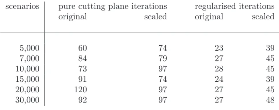
1. The computational behaviour: we solved the two models using their cutting plane representations (section 4.1) with the methods described in Section 5, i.e. the pure cutting plane method and the level method. We compared the number of iterations required in order to reach²optimality.
2. The modelling aspect: we analyse the return distributions of the portfolio solutions of (2) and (4) respectively.
6.1 Implementation issues
The methods were implemented using the AMPL modelling system (Fourer, Gay and Kernighan 1989) and the AMPL COM Component Library (Sadki 2005), integrated with C functions. Under AMPL we use the FortMP solver. FortMP was developed at Brunel University and NAG Ltd by Ellison et al. (1999), the project being co-ordinated by E.F.D. Ellison.
In our cutting-plane system, cut generation is implemented in C, and cutting-plane model problem data are forwarded to AMPL in each iteration. Hence the bulk of the arithmetic computations is done in C, since the number of the scenarios is typically large as compared to the number of the assets. Moreover, our test results imply that acceptable accuracy can be achieved by a relatively small number of cuts in the master problem. Hence the sizes of the model problems do not directly depend on the number of scenarios.
The methods were terminated when the difference between the upper and lower bounds on the objective functionϕ(x) became less or equal to the specified absolute tolerance².
scenarios pure cutting plane iterations regularised iterations
original scaled original scaled
5,000 60 74 23 39
7,000 84 79 27 45
10,000 73 97 28 45
15,000 91 74 24 39
20,000 120 97 27 45
30,000 92 97 27 48
Table 1: Iteration counts
Even though the implementation of the methods leaves many possibilities for speed-up, the performance of the methods was reasonably good. Even the largest problems with 30000 scenarios were solved within 1 minute on a computer with 1.73 GHz Intel Core Duo CPU and 2 GB of RAM running Windows XP.
6.2 Test problems
We generated scenario sets using Geometric Brownian Motion (GBM), which is standard in finance for modelling asset prices, see e.g., Ross (2002). Parameters for scenario generation were derived from a data set of 132 historical monthly returns of 76 stocks (all the stocks that belonged to the FTSE 100 during the period January 1993 - December 2003).
For reference return R, we used the FTSE 100 index. Scenario sets for the FTSE 100 monthly returnb were generated in the same way (using GBM and and historical returns of the index between January 1993 - December 2003).
We tested with different scenario sets, each containing up to 30000 scenarios. (A single scenario consists of 77 return values: one for each of the 76 component stocks, and one for the FTSE 100 index.)
6.3 Analysis of test results
In the first experiment, we compared the solution methods. We counted the iterations the different methods made until reaching²-optimal solutions. Typical iteration counts are cited in Table 1. (They were obtained with stopping tolerance set to²= 1e−7, and the level parameter set to 0.5.) It can be seen that regularisation substantially decreases the number of iterations.
In the second experiment, given a scenario set, we solved both problems (the ”original” model (2) and the ”scaled” model (4)) and compared the return distributions of the optimal portfolios. We made several comparisons with similar results. Basically, the proposed scaled tail model results in a return distribution that is mostly shifted to the right, as compared to the return distribution of the ”original” model (i.e. the model proposed by Roman, Darby-Dowman and Mitra).
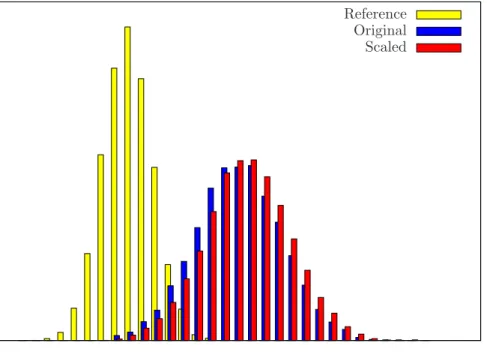
Figure 1 depicts the histograms of the return distributions obtained, for the case of the 30000-scenario problem, using the historical dataset described at the previous section (January 1993 - December 2003). The
”original” distribution (in blue) is the return distribution of the portfolio obtained with model (2) of Roman, Darby-Dowman and Mitra). The ”scaled” distribution (in red) is the return distribution of the portfolio obtained with the presently proposed model (4). The yellow histogram represents the reference distribution, of the FTSE 100 index.
The first two distributions clearly dominate the reference FTSE 100 distribution.
The ”scaled” distribution is mostly ”shifted to the right”, as compared to the ”original” distribution.
We underline that none of these distributions (”scaled” and ”original”) dominates the other; they are both
Reference Original Scaled
Figure 1: Dataset Jan 1993 - Dec 2003. Histograms for the return distributions of the optimal portfolios of SSD based models (”original” and ”scaled”) and for the FTSE100 Index (”reference”)
non-dominated with respect to SSD. The ”original” distribution (in blue) has a slightly better ”worst- case outcome” than the ”scaled” distribution (there is an invisible red bin situated at the left of the blue histogram). However, the ”scaled” distribution has in most cases larger numbers of outcomes in the bins situated at the right.
The scaled distribution has a higher mean at no expense on the standard deviation - Table 2 presents statistics of the three return distributions considered.
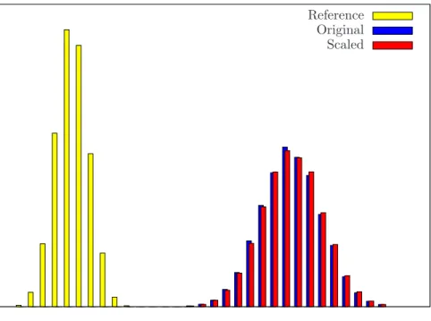
We repeated the tests using scenario sets constructed from different historical datasets. A 30,000 scenarios set has been created using a dataset of 70 stocks from FTSE 100 (plus the FTSE 100 index itself) with prices monitored monthly from Dec 1992 to Apr 2000 (the results are displayed in Figure 2).
A similar dataset, but with prices monitored monthly from May 2000 to Sep 2007, was used for generating a further 30,000 scenarios set (the results are displayed in Figure 3).
In all cases the ”scaled” distribution is mostly shifted to the right; exception makes only a very small part of the left tails. Although the worst-scenario outcomes are slightly better in the case of the ”original”
distribution, the vast majority of outcomes (and the mean value) are better for the ”scaled” distribution.
We believe that an investor would prefer the ”scaled” distribution (red histogram).
7 Discussion and conclusions
In this paper we have proposed an enhanced version of the SSD-based portfolio-selection model of Roman, Darby-Dowman and Mitra (2006). The present approach is based on comparison of the scaled tails of the distributions. This approach has advantages both from a theoretical and a practical perspective.
The enhanced model can be also formulated as a risk minimisation model using a convex risk measure.
Moreover, the new model offers a natural generalisation of the SSD-constrained formulation of Dentcheva and Ruszczy´nski (2006).
Our empirical study reveals that the enhanced model leads to portfolios with return distributions superior
original scaled index
Mean 0.0115 0.0121 0.0034
Median 0.0115 0.0121 0.0034
Standard Deviation 0.0032 0.0032 0.0018 Excess Kurtosis -0.0441 -0.0147 -0.0267 Skewness 0.0318 0.0236 0.0100
Range 0.0215 0.0232 0.0136
Minimum 0.0023 0.0017 -0.0034 Maximum 0.0238 0.0250 0.0102 Table 2: Statistics of the three return distributions considered
Reference Original Scaled
Figure 2: Dataset Dec 1992 - Apr 2000. Histograms for the return distributions of the optimal portfolios of
”original” and ”scaled” models and for the FTSE100 Index (”reference”)
Reference Original Scaled
Figure 3: Dataset May 2000 - Sep 2007. Histograms for the return distributions of the optimal portfolios of
”original” and ”scaled” models and for the FTSE100 Index (”reference”)
to those obtained by the model of Roman, Darby-Dowman and Mitra. The salient feature of the enhanced model is that the new return distributions are mostly shifted to the right, in relation to the original model.
The enhanced model is formulated constructively using a cutting plane representation and we have com- pared solution methods. The level method has proven more effective than the pure cutting-plane method, and the former method showed better scale-up properties. We have solved problems with tens of thousands of scenarios; in all cases, the solution time was less than one minute.
Acknowledgements
The authors would like to acknowledge the support for this research from several sources.
Professor Csaba F´abi´an’s research has been supported by OTKA, Hungarian National Fund for Scientific Research, project No. 47340, and by the Mobile Innovation Centre of the Budapest University of Technol- ogy, integrated project No. 2.2. Professor Csaba F´abi´an’s visit to CARISMA was supported by OptiRisk Systems, Uxbridge, UK and by BRIEF (Brunel University Research Innovation and Enterprise Fund).
Dr Diana Roman’s contribution to this work was supported by BRIEF (Brunel University Research Innova- tion and Enterprise Fund). The PhD studies of Victor Zverovich have been supported by OptiRisk Systems.
These sources of support are gratefully acknowledged.
References
[1] Artzner, Ph., F. Delbaen,J.-M. Eber, andD. Heath(1999). Coherent measures of risk.Math- ematical Finance 9203-227.
[2] Carr, P., H. Geman, andD. Madan(2001). Pricing and hedging in incomplete markets.Journal of Financial Economics62 131-167.
[3] Delbaen, F.(2002) Coherent risk measures on general probability spaces.Essays in Honour of Dieter Sondermann. Springer-Verlag, Berlin, Germany.
[4] Dempster, M.A.H. and R.R. Merkovsky (1995). A practical geometrically convergent cutting plane algorithm.SIAM Journal on Numerical Analysis 32, 631-644.
[5] Dentcheva, D.and A. Ruszczy´nski (2003). Optimization with stochastic dominance constraints.
SIAM Journal on Optimization 14, 548-566.
[6] Dentcheva, D.andA. Ruszczy´nski(2006). Portfolio optimization with stochastic dominance con- straints.Journal of Banking & Finance 30, 433-451.
[7] Ellison, E.F.D., M. Hajian, R. Levkovitz, I. Maros, and G. Mitra (1999). A Fortan based mathematical programming system FortMP. Brunel University, Uxbridge, UK and NAG Ltd, Oxford UK.
[8] F´abi´an, C.I., G. Mitra, and D. Roman (2008). Processing Second-Order Stochastic Dominance models using cutting-plane representations.Stochastic Programming E-Print Series 2008-10.
[9] F´abi´an, C.I. and Z. Sz˝oke (2007). Solving two-stage stochastic programming problems with level decomposition,Computational Management Science 4, 313-353.
[10] F¨ollmer, H.and A. Schied(2002). Convex measures of risk and trading constraints. Finance and Stochastics6429-447.
[11] Fourer, R., D. M. Gay, andB. Kernighan. (1989).AMPL: A Mathematical Programming Lan- guage.
[12] Hadar, J. andW. Russel(1969). Rules for ordering uncertain prospects.The American Economic Review 5925-34.
[13] Heath, D.(2000). Back to the future.Plenary Lecture at the First World Congress of the Bachelier Society, Paris, June 2000.
[14] Klein Haneveld, W.K.andM.H. van der Vlerk(2006). Integrated chance constraints: reduced forms and an algorithm.Computational Management Science 3, 245-269.
[15] Kroll, Y. andH. Levy (1980). Stochastic dominance: A review and some new evidence.Research in Finance 2, 163-227.
[16] K¨unzi-Bay, A.andJ. Mayer(2006). Computational aspects of minimizing conditional value-at-risk.
Computational Management Science 3, 3-27.
[17] Lemar´echal, C., A. Nemirovskii, and Yu. Nesterov(1995). New variants of bundle methods.
Mathematical Programming 69, 111-147.
[18] Ogryczak, W. and A. Ruszczy´nski (2001). On consistency of stochastic dominance and mean- semideviations models.Mathematical Programming 89, 217-232.
[19] Ogryczak, W.andA. Ruszczy´nski(2002). Dual stochastic dominance and related mean-risk mod- els.SIAM Journal on Optimization 13, 60-78.
[20] Rockafellar, R.T.(2007). Coherent approaches to risk in optimization under uncertainty.Tutorials in Operations Research INFORMS 2007, 38-61.
[21] Rockafellar, R.T. and S. Uryasev (2000). Optimization of conditional value-at-risk.Journal of Risk 2, 21-41.
[22] Rockafellar, R.T.andS. Uryasev(2002). Conditional value-at-risk for general loss distributions.
Journal of Banking & Finance 26, 1443-1471.
[23] Rockafellar, R. T., S. Uryasev, andM. Zabarankin(2002). Deviation measures in risk anal- ysis and optimization. Research Report 2002-7, Department of Industrial and Systems Engineering, University of Florida.
[24] Rockafellar, R. T., S. Uryasev, and M. Zabarankin (2006). Generalised deviations in risk analysis. Finance and Stochastics 10, 5174.
[25] Roman, D., K. Darby-Dowman, andG. Mitra(2006). Portfolio construction based on stochastic dominance and target return distributions.Mathematical Programming Series B 108, 541-569.
[26] Ross, S.M. (2002). An Elementary Introduction to Mathematical Finance. Cambridge University Press.
[27] Ruszczy´nski, A. and A. Shapiro (2006). Optimization of convex risk functions. Mathematics of Operations Research 31, 433452.
[28] Sadki, A.M.(2005). AMPL COM Component Library, User’s Guide Version 1.6.Internal T. Report.
See also http://www.optirik-systems.com/products/AMPLCOM.
[29] Whitmore, G.A. and M.C. Findlay (1978). Stochastic Dominance: An Approach to Decision- Making Under Risk. D.C.Heath, Lexington, MA.