Quantifying Systemic Risk by Solutions of the Mean-Variance Risk Model

(1)

Quantifying Systemic Risk by Solutions of the Mean-Variance Risk Model

Jan Jurczyk*^☯, Alexander Eckrot^☯, Ingo Morgenstern Department of Physics, University of Regensburg, Regensburg, Germany

☯These authors contributed equally to this work.

*jan.jurczyk@ur.de

Abstract

The world is still recovering from the financial crisis peaking in September 2008. The triggering event was the bankruptcy of Lehman Brothers. To detect such turmoils, one can investi- gate the time-dependent behaviour of correlations between assets or indices. These cross- correlations have been connected to the systemic risks within markets by several studies in the aftermath of this crisis. We study 37 different US indices which cover almost all aspects of the US economy and show that monitoring an average investor’s behaviour can be used to quantify times of increased risk. In this paper the overall investing strategy is approxi- mated by the ground-states of the mean-variance model along the efficient frontier bound to real world constraints. Changes in the behaviour of the average investor is utlilized as a early warning sign.

Introduction

Systemic risk is a financial term used to describe the probability of a breakdown in an entire system [1,2]. A typical example is a bank run, where a large number of bank clients decide to withdraw all their deposits at the same time. Consequently the bank is unable to fulfil contracts with other market participants or banks which leads to shortfalls in other sectors triggering a cascade of failures and a system-wide breakdown. In the last decade two major systemic risks lead to political and financial crisis, the global crisis in 2008 and the ongoing European debt crisis. The latter in combination with the inability of certain European states to place govern- ment bonds on the international market lead to the breakdown probability of the EURO-Zone.

In their study from 2010, Billio et al. [3] proposed that the two largest eigenvalues can be used to measure the underlying systemic risk of hedge funds, banks, brokers and insurance companies. In addition they used the Granger-Causality-Test [4] to illustrate the relation between these market sectors [3,5]. These studies showed the increasing entanglement of the big four in financial markets. By this, they outlined a predictive indicator to systemic risk. The study also states that the banking and hedge fund sector seize dominant roles. This idea was advanced by Zheng et al. in 2012 by using principle component analysis on a correlation matrix consisting of 10 US sector indices. They showed that the steepest increase in the first four largest eigenvalues is connected to the systemic risk of the chosen indices. At the same time, the a11111

OPEN ACCESS

Citation:Jurczyk J, Eckrot A, Morgenstern I (2016) Quantifying Systemic Risk by Solutions of the Mean- Variance Risk Model. PLoS ONE 11(6): e0158444.

doi:10.1371/journal.pone.0158444

Editor:Wei-Xing Zhou, East China University of Science and Technology, CHINA

Received:February 22, 2016 Accepted:June 16, 2016 Published:June 28, 2016

Copyright:© 2016 Jurczyk et al. This is an open access article distributed under the terms of the Creative Commons Attribution License, which permits unrestricted use, distribution, and reproduction in any medium, provided the original author and source are credited.

Data Availability Statement:All relevant data are within the paper and its Supporting Information files.

Funding:The authors have no support or funding to report.

Competing Interests:The authors have declared that no competing interests exist.

(2)

change in the four largest eigenvalues can be used as a precursor indicator. The magnitude of the increase translates to a higher interconnectedness of the 10 US sector indices and its risk aversion. [6,7]

Former studies based their measure of systemic risk upon the relation between banks [8–13]

and others focused more on time-series analysis with different risk-measures [9,14–19]. The idea of news contagion is starting to become a part of systemic risk analysis [20–22]. We suggest that when studying systemic risks, one also has to take market participants behaviour, like banks, into account. The investors general goal is to generate return with a low risk exposure.

The mean-variance model by Markowitz [23] was the first model capturing this need. There- fore we connect the ground-state portfolios spanning the efficient frontier to systemic risks [24]. A sharp change in the suggested portfolio is connected to the search of a new low overall risk. When all market participants are in that state the breakdown probability increases due to their increased connectivity [25]. The problem of selecting the optimal portfolio composition translates to the risks within the underlying dataset. An increase in the number of negative options correlates to a higher breakdown probability of the monitored dataset, since the number of stable configurations decreases. In this paper we introduce a measure called investing strategyM, which approximates the market participants behaviour by the ground-states of the mean-variance model with real world constraints. The time derivative of the average investing strategy peaks at the global financial crisis of 2008, the EURO-dept crisis and the Chinese stock market crash in 2015.

Methods

The mean-variance model

The mean-variance model was introduced by Markowitz in 1952 [23] and is one of the corner- stones of modern portfolio theory [26]. The objective is to maximise the average portfolio return

R_P¼X^N

i¼1

r_ip_i ð1Þ

of portfolio weightsP= (p1,p2,. . .,pN)^Twith expected returnsrifor each assetiand minimise its variance

var_P¼X

i;j

p_iC_ijp_j ð2Þ

with the covariance matrixCij. Both the covariance matrix and the expected returns are calculated from logarithmic returns

r_iðtÞ ¼ logðPriceiðtÞÞ logðPriceiðt1ÞÞ ð3Þ wheretdenotes the time and runs through a single periodO= {t|T−ωtT} with lagωand theﬁnal datapoint at timeT. The classical approach is constraining the portfolio to positive val- uespi08iand therefore preventing short-selling positions. Since an investor is bound by his available budget, all portfolio weights must sum up to one. This model quantiﬁes the risk of a selected portfolio by using the variance and balances it with the expected return. Therefore an investor is able to choose a portfolio with the highest possible return at a certain risk level [27].

From an investors point of view, the classical model is not capturing real world demands of maintaining a portfolio. When constructing a portfolio, one has to account for transaction costs, which manifest in the cardinality of a portfolio. The three main constrictions a real

(3)

investor has to consider [28], are the buy-in thresholdτ, which defines a level of minimal investment in any asseti; the base unit of investmentz; and the cardinality constraintNd, which sets the number of desired assets an investor wishes to manage. Introducing these real world demands to the model, it develops the portfolio selection problem from a quadratic programming problem to a NP-complete problem [29]. Due to the practical implications of portfolio managing, the cardinality constraint portfolio selection problem has been researched extensively [26,28–39]. Under real market conditions an investor can profit from a decline in stock prices by purchasing short-options. Including this extension, every portfolio has to fulfil

X

i

jpij ¼1 ð4Þ

when cycling throughO. This evolves the budget constraint to negative portfolio options, under the restriction not to invest over-proportionally in declining prices. The objective function

H¼ lR_Pþ ð1lÞvar_P ð5Þ

whereRPcorresponds to the portfolio return and var_Pto its variance, is minimised under the constraints of budget, cardinality and buy-in. In the context of portfolio selection, the parameter λcontrols the level of risk one is willing to accept for a certain amount of returnRP. This non trivial optimisation problem is solved by a tailored simulated annealing algorithm [40].

The investing strategy

A general investing strategyMis based on the efficient frontier (EF), which is constructed by varying the parameterλfrom 0 to 1 where for eachλan optimal or ground-state portfolioP exists with a tuple (var_P,RP) on the risk return plane. To quantify the investing strategyM, the sum of allP_iis used, which is similar to a physical magnetisation [41] and weighted with a density functionρ(λ)

M_rðT;oÞ ¼C¹Z¹

0

dl rðlÞX^N

i¼1

P_iðl;T;oÞ ¼C¹Z 1

0 dlrðlÞ mðl;T;oÞ ð6Þ withC¼R1

0 dlrðlÞas a scaling constant. Therefore the investing strategyMindicates which proportion of portfolios along the efﬁcient frontier, based upon the chosen density functionρ, should be invested into shorts or longs. The lagged time derivative

@tlMðTÞ ¼MðTÞ MðTlÞ ð7Þ measures the changes in the investing strategy between two points in timeTseparated byl time-units.

A change in the behaviour of an average investor can be used as an early warning sign [42].

This idea is exploited byEq (6). Since one does not know every market participant and their investments, the investing strategy approximates the investor ensemble by the ground-state P(λ) for a certain risk-level. A shift in the ground-states along the EF leads to an overall changed market sentiment and therefore investors have to reevaluate their investments. In terms of a phase transition, a new basin is emerging and system participants, who are effec- tively sampling the market, will start to occupy that state [25,42]. To move to the new state investors have to sell and buy new assets, which results in a higher trading volume, which in turn is connected to a higher volatility [43]. Assuming that investors are bound to the constraints introduced above, it is possible to detect such periods by monitoring the changes in the investing strategy inEq (7)

(4)

Data

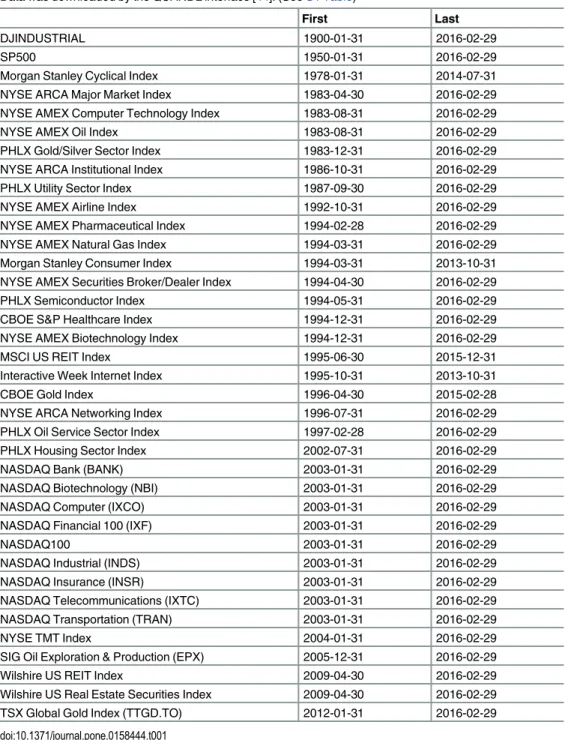
All 37 US indices (Table 1) were downloaded by the QUANDL [44] interface. If for an observed time-frameOdata is missing, the whole index is omitted for the analysis of the EF and its corresponding investing strategy. This is done in order to replicate the choices an investor has at a certain time with a given set of parameters.

Table 1. List of all US indices used to calculate the efficient frontier and their available time-frames.All Data was downloaded by the QUANDL interface [44]. (SeeS1 Table)

First Last

DJINDUSTRIAL 1900-01-31 2016-02-29

SP500 1950-01-31 2016-02-29

Morgan Stanley Cyclical Index 1978-01-31 2014-07-31

NYSE ARCA Major Market Index 1983-04-30 2016-02-29

NYSE AMEX Computer Technology Index 1983-08-31 2016-02-29

NYSE AMEX Oil Index 1983-08-31 2016-02-29

PHLX Gold/Silver Sector Index 1983-12-31 2016-02-29

NYSE ARCA Institutional Index 1986-10-31 2016-02-29

PHLX Utility Sector Index 1987-09-30 2016-02-29

NYSE AMEX Airline Index 1992-10-31 2016-02-29

NYSE AMEX Pharmaceutical Index 1994-02-28 2016-02-29

NYSE AMEX Natural Gas Index 1994-03-31 2016-02-29

Morgan Stanley Consumer Index 1994-03-31 2013-10-31

NYSE AMEX Securities Broker/Dealer Index 1994-04-30 2016-02-29

PHLX Semiconductor Index 1994-05-31 2016-02-29

CBOE S&P Healthcare Index 1994-12-31 2016-02-29

NYSE AMEX Biotechnology Index 1994-12-31 2016-02-29

MSCI US REIT Index 1995-06-30 2015-12-31

Interactive Week Internet Index 1995-10-31 2013-10-31

CBOE Gold Index 1996-04-30 2015-02-28

NYSE ARCA Networking Index 1996-07-31 2016-02-29

PHLX Oil Service Sector Index 1997-02-28 2016-02-29

PHLX Housing Sector Index 2002-07-31 2016-02-29

NASDAQ Bank (BANK) 2003-01-31 2016-02-29

NASDAQ Biotechnology (NBI) 2003-01-31 2016-02-29

NASDAQ Computer (IXCO) 2003-01-31 2016-02-29

NASDAQ Financial 100 (IXF) 2003-01-31 2016-02-29

NASDAQ100 2003-01-31 2016-02-29

NASDAQ Industrial (INDS) 2003-01-31 2016-02-29

NASDAQ Insurance (INSR) 2003-01-31 2016-02-29

NASDAQ Telecommunications (IXTC) 2003-01-31 2016-02-29

NASDAQ Transportation (TRAN) 2003-01-31 2016-02-29

NYSE TMT Index 2004-01-31 2016-02-29

SIG Oil Exploration & Production (EPX) 2005-12-31 2016-02-29

Wilshire US REIT Index 2009-04-30 2016-02-29

Wilshire US Real Estate Securities Index 2009-04-30 2016-02-29

TSX Global Gold Index (TTGD.TO) 2012-01-31 2016-02-29

doi:10.1371/journal.pone.0158444.t001

(5)

Results and Discussion

In order to show thatMis a possible early warning sign, we calculate the logarithmic monthly returns of 37 US indices and solve the portfolio selection problem (PSP) under the constraints that the portfolio has to consist ofNd= 5 indices and the buy-inτas well as the base unit of investmentzis set to 10⁻⁴. The efficient frontier is constructed byn= 501 differentλ’s equidis- tant distributed from 0 to 1. In order to capture the average over the efficient frontier,ρ(λ) is set to a constant value. We note that the given parameters are common values used in cardinality constraint optimisation problems, but we also tested different sets of parameters and density distributionsρwith similar results (seeS1 Text).

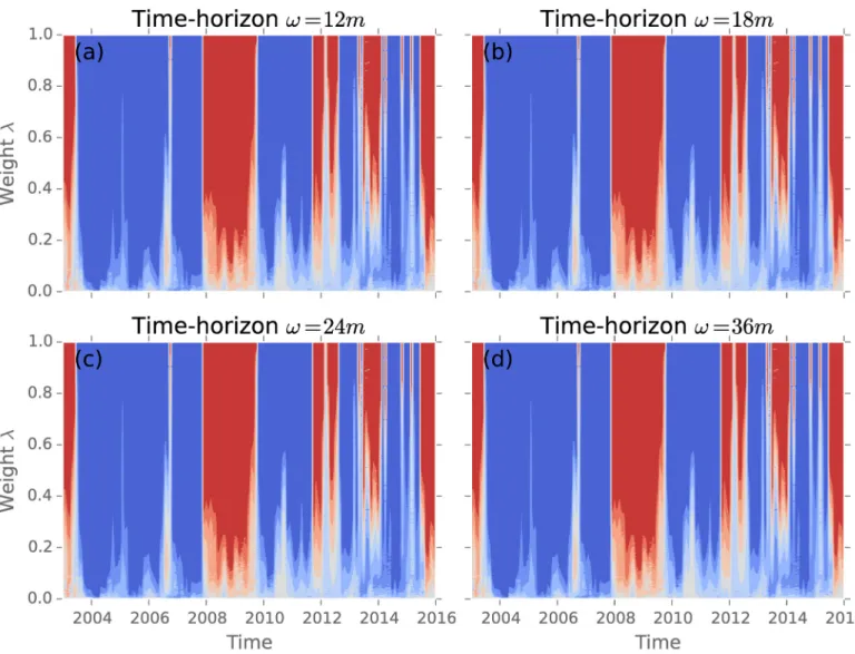
Fig 1shows the time-development of the suggested investment strategiesm(t,λ) starting in 2003. These are deduced from the mean-variance model with different time-horizonsω. Blue colours represent stable phases with mostly positive weights, while red colours indicate phases with high systemic risk, due to a large negative weight proportion. In all depicted time-horizons, the global financial crisis is present from 2007 until 2009. The longer the time-horizons,

Fig 1. The investing strategies calculated for different time-horizons from January 2003 until January 2016.(a)ω= 1 year; (b)ω= 18 months;

(c)ω= 2yand (d)ω= 3y; Blue signals a majority of positive portfolio weights, while red is related to dominantly negative weights in the solution. In all time-windows (a)-(d) the global financial crisis is depicted with negative weights.

doi:10.1371/journal.pone.0158444.g001

(6)

the longer it takes to recover to stable conditions. Optimal portfolios are dependent on the time-horizon, since a different time-horizonωresults in a divers set of returns [28].

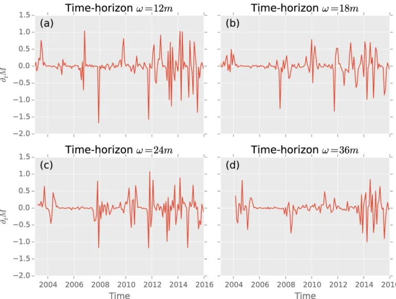
We show dependence on time inFig 2, starting with a time-horizon of 12-month up to 36-month. These time-horizons are usually used in literature [3,6,14,30]. For the purpose of this paper, we chose our observation time-horizon to beω= 12months, since it exhibits the most distinctive peaks. Choosing a largerωleads to a smoothing of the signal, since shocks happen on a shorter time-scales and loose their impact on the statistics over longer times. [6]

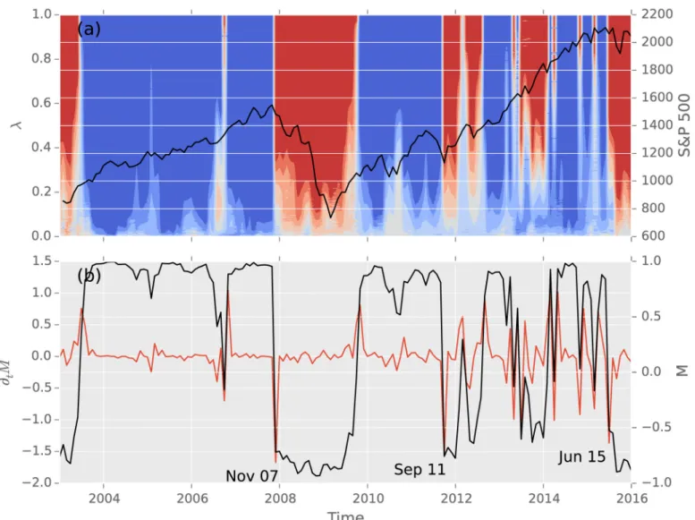
In November 2007, the average investing strategyM(t) dropped from 95% to−73% (seeFig 3). This decrease by@tM=−168% is the largest drop in the 12 month time-horizon as well as in the observation time starting in 2003. AfterwardsMkept decreasing to the minimum ofM=

−94%, after recovering in October 2009. During this time of financial turmoils, the average investing strategy was ranging between−57% and−94%. In September 2011 a slump of@tM=−157%

occurred. This corresponds to the time where speculation about the survival of the EURO-Zone took place. In this crisis the average investing strategy never drops below−77%. The next largest

Fig 2. (a)–(d) depict the time derivation of the average investing strategies for different time-horizons.In (a) withω= 1 year the three major crisis in the time from 2003 until 2016 exhibit the three largest drops. On longer time-horizons (b)ω= 18 months, (c)ω= 2 years and (d)ω= 3 years many signals mix and the decreases are not highly developed. Especially since 2013 volatility clustering is observed.

(7)

decline is observed in June 2015 with@tM=−136%. Over the following months the average investing strategy was slipping up toM=−90% in January 2016. During this timeframe, the Chi- nese market was suffering from turmoils. A drop to these values has not been seen since the financial crisis.

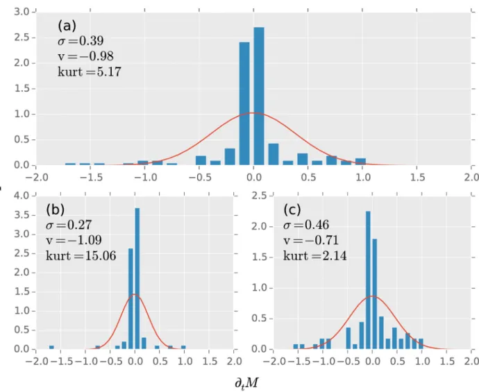
Next we study the behaviour of the changes in average investment strategy on a twelve month time-horizon before and after the financial crisis (Fig 4). We select the up-move from unstable to stable in October 2009 as the separating point of the two studied time-periods. The overall probability density function (Fig 4a) from 2003 to 2016 is skewed with v =−0.98. In comparison with the normal distribution with the same standard deviationσ= 0.39 a non van- ishing probability of extreme events exit. We suggest, that these fat tails are related to the systemic risk.

Separating the time-series into two parts, before (Fig 4b) and after October 2009 (Fig 4c), we observe a difference in the kurtosis from kurt = 15.06 to kurt = 2.14. During the time before

Fig 3. Comparison of the average investing strategy and its recordings with the S&P 500 index, in theω= 12 months time-horizon.(a) shows the heat-map with varying risk levelλon the left y-axis and the logarithmic values of the S&P 500 index on the right y-axis. (b) shows on the left the changes in the average investing strategy (right y-axis). The slumps in November 2007, September 2011 and June 2015 fall in the times of sub-prime/

financial crisis, EURO-Zone debt crisis and Chinese stock market crash.

(8)

October 2009, the distribution is dominated by the outliers around the meanh@tMi −0.00.

While the skewness remains with v =−1.09 before and v =−0.71 after in the same range, the standard deviation almost doubles fromσ= 0.27 toσ= 0.46.

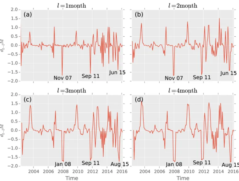
In order to quantify the highest peak,Fig 5shows a time-derivative with different lags defined by

@_tlM¼MðtÞ MðtlÞ: ð8Þ

The sharpest change occurs in the derivative withl= 1 month in October 2007, which also marks the highest peak in the S&P 500 in its history. Increasing the laglto higher values the peak broadens since after a drop the magnitude can increase. We find that inFig 5a and 5bthe absolute peak occurs in November 2007, while with longer lagsl= 3, 4 months inFig 5c and 5d

Fig 4. The average investing strategy time derivation probability functions (pdf) of (a) the whole observation time from 2003 until 2016; (b) from 2003 until 2009; and (c) from 2009 until 2016.Between 2003 and 2009 the pdf densely centered aroundh@tMi=

−0.00±0.04 exhibiting a kurt = 15.06±1.07 and an extreme event at−1.5. Afterwards theh@tMi=−0.00±0.05 is also centered. The kurtosis dropped to kurt = 2.14±1.07 and shows a standard deviation ofσ= 0.46±0.05 in comparison toσ= 0.27±0.08. The skewness changed from v =−1.09±2.44 before 2009 and v =−0.71±0.36. The whole observation time pdf hash@tMi=−0.00±0.03 withσ= 0.39±0.04, kurt = 5.17±1.60 and v =−0.98±0.50. Note, that these values were estimated with 1000 bootstrapping samples. The comparison plot is a normal distribution with zero mean and the corresponding standard deviations for each time frame.

(9)

the peak is found in January 2008. Similarly the last large decrease is found in June 2015 (Fig 5a and 5b) or in August 2015 (Fig 5a and 5b).

Due to globalisation processes, financial markets have become more entangled in the last 25 years. Thus the cross-correlation between markets and sectors increased [45–47], which makes the sectors more suggestible to events in others. This cascading is connected to systemic risks.

This paper proposes that systemic risk can be quantified by the behaviour of the average investment strategy of a portfolio selection problem. Abrupt changes signal that the stable configura- tion has to adapt to changing market situations. Since every investor has to balance return with risk, one can track these financial reflections ahead of time. We showed that the 12 month win- dow of monthly log returns is a suitable parameter range. Since the optimal solutions found translate to the most efficient way of investing, according to Markowitz, they trace the general market behaviour. Therefore our indicator can be used on large data sets with many different economic sectors and needs no selection process before hand.Fig 3displays the investing strategies, its average and time-derivative and compares it to the log values of the S&P 500. Besides

Fig 5. The three largest drops in time derivation with lag (a)l= 1 month, (b)l= 1 month, (c)l= 3 month and (d)l= 4 month of the average investing strategy in the time-horizonω= 12months.With lagl= 1, 2 these occur ordered by strength November 2007, September 2011 and June 20015. Lagl= 3, 4 this changes to August 2015, January 2008 and September 2011.

(10)

the negative phase between November 2007 and October 2009, a new phase has formed in June of 2015. The latter may be connected to the Chinese stock market crash. The evaluated time-frame shows that the three major crisis, which took place are the three greatest decreases in the average investing strategy.

The fluctuations present between October 2009 and June 2015, are in our opinion due to high uncertainties. It is not possible to settle into a phase for a long time period. In analogy to physics, this is present when a magnet is at critical temperature. Despite the high fluctuations, the absolute value of the average investing strategy does not drop belowM=−60%, while in the financial crisis this value was well undershot.

In conclusion, we propose that sharp changes in the investing strategies, relying on the efficient frontier by Markowitz, serve as an indicator for systemic risks which can cascade to all market sectors of an economy.

Supporting Information

S1 Text. Effect ofρon the AIS with a comparison to an eigenvalue analysis.

(PDF)

S1 Table. List of QUANDL Codes used.

(CSV)

Author Contributions

Conceived and designed the experiments: JJ. Performed the experiments: JJ. Analyzed the data:

JJ AE IM. Wrote the paper: JJ AE.

References

1. Kaufman GG, Scott KE. What is Systemic Risk, and Do Banks Regulators Retard or Contribute to It?

The Independent Review. 2003; 3(3):371.

2. Kaufman GG. Banking and Currency Crisis and Systemic Risk: A Taxonomy and Review. Financial Markets, Institutions and Instruments. 2000 may; 9(2):69–131. doi:10.1111/1468-0416.00036 3. Billio M, Getmansky M, Lo A. Measuring systemic risk in the finance and insurance sectors. NBER

working paper. 2010 jul;

4. Granger CWJ. Testing for causality. Journal of Economic Dynamics and Control. 1980 jan; 2:329–352.

doi:10.1016/0165-1889(80)90069-X

5. Billio M, Getmansky M, Lo AW, Pelizzon L. Econometric measures of connectedness and systemic risk in the finance and insurance sectors. Journal of Financial Economics. 2012 jun; 104(3):535–559. doi:

10.1016/j.jfineco.2011.12.010

6. Zheng Z, Podobnik B, Feng L, Li B. Changes in cross-correlations as an indicator for systemic risk. Sci- entific reports. 2012 nov; 2:888. doi:10.1038/srep00888PMID:23185692

7. Kritzman M, Li Y, Page S, Rigobon R. Principal Components as a Measure of Systemic Risk. The Jour- nal of Portfolio Management. 2011; 37(4):112–126. doi:10.3905/jpm.2011.37.4.112

8. Lehar A. Measuring systemic risk: A risk management approach. Journal of Banking & Finance. 2005;

29(10):2577–2603. doi:10.1016/j.jbankfin.2004.09.007

9. Pérignon C, Deng ZY, Wang ZJ. Do banks overstate their Value-at-Risk? Journal of Banking &

Finance. 2008 may; 32(5):783–794. doi:10.1016/j.jbankfin.2007.05.014

10. Langfield S, Pagano M. Bank Bias in Europe: Effects on Systemic Risk and Growth. Economic Policy.

2016;. doi:10.1093/epolic/eiv019

11. Pais A, Stork PA. Bank size and systemic risk. European Financial Management. 2013; 19(3):429– 451. doi:10.1111/j.1468-036X.2010.00603.x

12. De Bandt O, Hartmann P. Systemic Risk: A Survey; 2000.

13. Haldane AG, May RM. Systemic risk in banking ecosystems. Nature. 2011 jan; 469(7330):351–5.

PMID:21248842

(11)

14. Bisias D, Flood MD, Lo AW, Valavanis S. A Survey of Systemic Risk Analytics. Annual Review of Financial Economics. 2012 jan; 4(1):255–296. doi:10.1146/annurev-financial-110311-101754 15. Rodríguez-Moreno M, Peña JI. Systemic risk measures: The simpler the better? Journal of Banking

and Finance. 2013 jun; 37(6):1817–1831. doi:10.1016/j.jbankfin.2012.07.010

16. Wang D, Podobnik B, HorvatićD, Stanley HE. Quantifying and modeling long-range cross correlations in multiple time series with applications to world stock indices. Physical Review E. 2011; 83(4):046121.

doi:10.1103/PhysRevE.83.046121

17. Wilcox D, Gebbie T. An analysis of cross-correlations in an emerging market. Physica A: Statistical Mechanics and its Applications. 2007; 375(2):584–598. doi:10.1016/j.physa.2006.10.030

18. Podobnik B, Wang D, Horvatic D, Grosse I, Stanley HE. Time-lag cross-correlations in collective phe- nomena. EPL (Europhysics Letters). 2010 jun; 90(6):68001. doi:10.1209/0295-5075/90/68001 19. Podobnik B, Horvatic D, Petersen AM, Stanley HE. Cross-correlations between volume change and

price change. Proceedings of the National Academy of Sciences of the United States of America. 2009 dec; 106(52):22079–84. doi:10.1073/pnas.0911983106PMID:20018772

20. Preis T, Moat HS, Stanley HE. Quantifying trading behavior in financial markets using Google Trends.

Scientific reports. 2013 jan; 3:1684. doi:10.1038/srep01684PMID:23619126

21. Moat HS, Curme C, Avakian A, Kenett DY, Stanley HE, Preis T. Quantifying Wikipedia Usage Patterns Before Stock Market Moves. Scientific Reports. 2013 may; 3:1801. doi:10.1038/srep01801

22. Huang X. Macroeconomic News Announcements, Systemic Risk, Financial Market Volatility and Jumps. Finance and Economics Discussion Series. 2015 oct; 2015(97):1–52.

23. Markowitz H. Portfolio Selection*. The Journal of Finance. 1952 mar; 7(1):77–91. doi:10.2307/

2975974

24. Jurczyk J. Measuring switching processes in financial markets with the Mean-Variance spin glass approach. 2015 mar;p. 7.

25. Scheffer M, Carpenter SR, Lenton TM, Bascompte J, Brock W, Dakos V, et al. Anticipating critical transitions. Science (New York, NY). 2012 oct; 338(6105):344–8. doi:10.1126/science.1225244

26. Cesarone F, Scozzari A, Tardella F. Efficient algorithms for mean-variance portfolio optimization with hard real-world constraints. Giornale dell’Istituto Italiano degli Attuari. 2009;p. 1–15.

27. Zhou XY. Continuous-Time Mean-Variance Portfolio Selection: A Stochastic LQ Framework. Applied Mathematics and Optimization. 2000 jul; 42(1):19–33. doi:10.1007/s002450010003

28. Jobst NJ, Horniman MD, Lucas CA, Mitra G. Computational aspects of alternative portfolio selection models in the presence of discrete asset choice constraints. Quantitative Finance. 2001; 1(5):489–501.

doi:10.1088/1469-7688/1/5/301

29. Di Gaspero L, di Tollo G, Roli A, Schaerf A. Hybrid Local Search for Constrained Financial Portfolio Selection Problems. Integration of AI and OR Techniques in Constraint Programming for Combinatorial Optimization Problems. 2007; 4510:44–58. doi:10.1007/978-3-540-72397-4_4

30. Cesarone F, Scozzari A, Tardella F. Portfolio selection problems in practice: a comparison between lin- ear and quadratic optimization models. arXiv preprint arXiv:11053594. 2011 may;p. 1–28.

31. Bienstock D. Computational study of a family of mixed-integer quadratic programming problems. Math- ematical Programming. 1996 aug; 74(2):121–140. doi:10.1016/0025-5610(96)00044-5

32. Chang TJ, Meade N, Beasley JE, Sharaiha YM. Heuristics for cardinality constrained portfolio optimisation. Computers and Operations Research. 2000; 27(13):1271–1302. doi:10.1016/S0305-0548(99) 00074-X

33. Crama Y, Schyns M. Simulated annealing for complex portfolio selection problems. European Journal of Operational Research. 2003 nov; 150(3):546–571. doi:10.1016/S0377-2217(02)00784-1 34. Fieldsend JE, Matatko J, Peng M. Cardinality constrained portfolio optimisation. In: Intelligent Data

Engineering and Automated Learning–IDEAL 2004. Springer; 2004. p. 788–793.

35. Mansini R, Speranza MG. Heuristic algorithms for the portfolio selection problem with minimum transaction lots. European Journal of Operational Research. 1999; 114(2):219–233. doi:10.1016/S0377- 2217(98)00252-5

36. Li D, Sun X, Wang J. Optimal lot solution to cardinality constrained mean-variance formulation for portfolio selection. Mathematical Finance. 2006 jan; 16(1):83–101. doi:10.1111/j.1467-9965.2006.00262.x 37. Maringer D, Kellerer H. Optimization of cardinality constrained portfolios with a hybrid local search algo-

rithm. OR Spectrum. 2003 oct; 25(4):481–495. doi:10.1007/s00291-003-0139-1

38. Schaerf A. Local Search Techniques for Constrained Portfolio Selection Problems. Computational Eco- nomics. 2002; 20(3):177–190. doi:10.1023/A:1020920706534

(12)

39. Streichert F, Ulmer H, Zell A. Evolutionary Algorithms and the Cardinality Constrained Portfolio Optimi- zation Problem. In: Operations Research Proceedings 2003, Selected Papers of the International Con- ference on Operations Research. Springer; 2003. p. 1–8.

40. Kirkpatrick S, Gelatt CD, Vecchi MP. Optimization by Simulated Annealing. Science. 1983 may; 220 (4598):671–80. doi:10.1126/science.220.4598.671PMID:17813860

41. Rosenow B, Plerou V, Gopikrishnan P, Stanley HE. Portfolio Optimization and the Random Magnet Problem. Europhysics Letters. 2002; 59(4):500–506. doi:10.1209/epl/i2002-00135-4

42. Levy M. Stock market crashes as social phase transitions. Journal of Economic Dynamics and Control.

2008 jan; 32(1):137–155. doi:10.1016/j.jedc.2007.01.023

43. Cont Rama Empirical properties of asset returns: stylized facts and statistical issues Taylor & Francis.

2001

44. Quandl. Quandl Financial and Economic Data;. Available from:https://www.quandl.com/.

45. Preis T, Kenett DY, Stanley HE, Helbing D, Ben-Jacob E. Quantifying the behavior of stock correlations under market stress. Scientific reports. 2012 jan; 2:752. doi:10.1038/srep00752PMID:23082242 46. King Mervyn, Sentana Enrique and Wadhwani S. Volatility and links between stock markets; 1990.

47. Solnik B, Boucrelle C, Le Fur Y. International Market Correlation and Volatility. Financial Analysts Jour- nal. 1996 sep; 52(5):17–34. doi:10.2469/faj.v52.n5.2021