doi: 10.3389/fmars.2018.00500
Edited by:
Laura Anne Bristow, University of Southern Denmark, Denmark
Reviewed by:
Brivaela Moriceau, UMR 6539, Laboratoire des Sciences de l’Environnement Marin (LEMAR), France Daniel Conrad Ogilvie Thornton, Texas A&M University, United States
*Correspondence:
Carolina Cisternas-Novoa ccisternas@geomar.de
†Present address:
Tiantian Tang, State Key Laboratory of Marine Environmental Science, Xiamen University, Xiamen, China Roman de Jesus, Earth Sciences Department, Fullerton College, Fullerton, CA, United States
Specialty section:
This article was submitted to Marine Biogeochemistry, a section of the journal Frontiers in Marine Science
Received:06 July 2018 Accepted:12 December 2018 Published:07 January 2019
Citation:
Cisternas-Novoa C, Lee C, Tang T, de Jesus R and Engel A (2019) Effects of Higher CO2 and Temperature on Exopolymer Particle Content and Physical Properties of Marine Aggregates.
Front. Mar. Sci. 5:500.
doi: 10.3389/fmars.2018.00500
Effects of Higher CO 2 and
Temperature on Exopolymer Particle Content and Physical Properties of Marine Aggregates
Carolina Cisternas-Novoa1,2* , Cindy Lee1, Tiantian Tang1†, Roman de Jesus1†and Anja Engel2
1School of Marine and Atmospheric Sciences, Stony Brook University, Stony Brook, NY, United States,2GEOMAR, Helmholtz Centre for Ocean Research Kiel, Kiel, Germany
We investigated how future ocean conditions, and specifically the interaction between temperature and CO2, might affect marine aggregate formation and physical properties.
Initially, mesocosms filled with coastal seawater were subjected to three different treatments of CO2concentration and temperature: (1) 750 ppm CO2, 16◦C, (2) 750 ppm CO2, 20◦C, and (3) 390 ppm CO2, 16◦C. Diatom-dominated phytoplankton blooms were induced in the mesocosms by addition of nutrients. In aggregates produced in roller tanks using seawater taken from the mesocosms during different stages of the bloom, we measured sinking velocity, size, chlorophyll a, particulate organic carbon and nitrogen, and exopolymer particle content; excess density and mass were calculated from the sinking velocity and size of the aggregates. As has been seen in previous experiments, no discernable differences in overall nutrient uptake, chlorophyll-a concentration, or exopolymer particle concentrations could be related to the acidification treatment in the mesocosms. In addition, in the aggregates formed during the roller tank experiments (RTEs), we observed no statistically significant differences in chemical composition among the treatments during Pre-Bloom, Bloom, and Post-Bloom periods.
However, physical characteristics were different and showed a synergistic effect of warmer temperature and higher CO2 during the Pre-Bloom period; at this time, temperature had a larger effect than CO2 on aggregate sinking velocity. In RTEs with warmer and acidified treatment (future conditions), aggregates were larger, heavier, and settled faster than aggregates formed at present-day or only acidified conditions. During the Post-Bloom, however, aggregates formed under present and future conditions had similar physical properties. In acidified tanks at ambient temperature, aggregates were slower, smaller and less dense than those formed at the same temperature but under present CO2 or under warmer and acidified conditions. Thus, the sinking velocity of aggregates formed in acidified tanks at ambient temperature was slower than the other two cases. Our findings point out the potential of ocean acidification and warming to modify physical properties of sinking aggregates but also emphasize the need of future experiments investigating multiple environmental stressors to clarify the importance of each factor.
Keywords: phytoplankton aggregates, aggregate sinking velocity, mesocosm, roller tank, transparent exopolymeric particles, Coomassie stainable particles
INTRODUCTION
The rise in atmospheric carbon dioxide (CO2) due to anthropogenic activities has led to increases in global temperature and ocean acidification. CO2has increased from 280 ppm in pre- industrial times to more than 400 ppm today. As a result of this increase, surface pH has decreased by 0.1 units and is expected to drop another 0.4 units by the year 2100 if the emissions continue as “business as usual” (IPCC, 2014). The ocean has absorbed one third of the total CO2emissions during the last century (Sabine et al., 2004). Globally, the temperature in the upper 75 m of the water column has increased by 0.09–0.13◦C per decade between 1971 and 2010 (IPCC, 2014). Elevated temperature and CO2 conditions affect rates of key phytoplankton processes, such as primary production (Rost et al., 2008; Egge et al., 2009;Engel et al., 2013), growth (Feng et al., 2008), calcification (Riebesell et al., 2000;Delille et al., 2005), nitrogen fixation (Karl et al., 2002;
Rost et al., 2008), and production of extracellular material (Engel, 2002;Kim et al., 2011;Engel et al., 2014).
Sinking particles, such as fecal pellets, aggregates, and other marine detritus, are the main vehicles for vertical transport and sequestration of carbon to the deep ocean (Alldredge and Jackson, 1995; Honjo et al., 2008; Turner, 2015). Aggregation of phytoplankton cells into sinking particles can be aided by the presence of highly sticky polysaccharide-rich transparent exopolymeric particles, or TEP (Alldredge et al., 1993). As oceanic CO2levels rise and pH falls, calcium carbonate saturation levels decrease (Doney et al., 2009). Lower CaCO3 saturation levels may lower the sinking velocity of marine aggregates and thus the efficiency of export due to a decrease in the ballast component (Armstrong et al., 2001; Klaas and Archer, 2002;
Biermann and Engel, 2010). On the other hand, under elevated CO2 conditions, both CO2 uptake (Riebesell et al., 2007) and DOC exudation by phytoplankton may increase (Borchard and Engel, 2012), leading to higher concentrations of TEP since they originate from dissolved precursors (Engel, 2002;Verdugo, 2012). Higher abundances of exopolymer particles, such as TEP might enhance aggregation and thus the particulate organic carbon (POC) flux into the deep ocean (Arrigo, 2007;Engel et al., 2014;Bourdin et al., 2017). However, not all studies have shown a direct relationship between elevated CO2levels and higher TEP production (Egge et al., 2009;Passow, 2012), or between higher TEP and greater aggregation and particle sinking (Seebah et al., 2014). To date, it is still unclear how ocean acidification and warming will affect TEP production and properties.
Another type of less studied exopolymer particles are the protein-rich Coomassie Blue stainable particles (CSP) (Long and Azam, 1996). It has been suggested that the role of CSP in aggregate formation varies depending on the dominant phytoplankton species; they may be relatively important for cyanobacteria aggregates (Cisternas-Novoa et al., 2015), but seem to play a less important role than TEP in diatom aggregates (Prieto et al., 2002;Cisternas-Novoa et al., 2015). There are no studies investigating how future ocean conditions may affect characteristics and concentrations of CSP and their role in the biogeochemical cycling of POC and particulate nitrogen (PN).
Responses of plankton species to increases in CO2
concentration (Riebesell et al., 2000, 2007; Eggers et al.,
2014;Schulz et al., 2017) and temperature (Claquin et al., 2008;
Edwards Kyle et al., 2016) have been examined in numerous manipulative experiments over the last two decades. An increasing number of studies have addressed the synergistic effects of warming and acidification on phytoplankton production (Borchard et al., 2011; Maugendre et al., 2015;
Sommer et al., 2015; Paul et al., 2016) and on organic matter production (Schulz et al., 2008;Kim et al., 2011;Borchard and Engel, 2012;Chen et al., 2015). To date, the combined effect of warming and acidification on TEP concentration and marine aggregates has been studied only on aggregates formed from Thalassiosira weissflogiigrown in batch cultures (Seebah et al., 2014).
Mesocosm experiments investigating effects of warming, or acidification and warming together, have shown an enhanced DOC: POC production ratio (Wohlers et al., 2009; Kim et al., 2011; Maugendre et al., 2017a), but how these findings relate to particle sinking and sequestration of organic carbon into the deep ocean have only been inferred and not directly measured.
Piontek et al. (2009)showed that elevated temperature increased not only aggregation, probably due to higher TEP concentrations, but also bacterial activity and remineralization, which could enhance carbon flux attenuation. Moreover, the effect of ocean acidification and warming on aggregation and carbon export may vary depending on the dominant phytoplankton groups (Eggers et al., 2014; Stange et al., 2018). Passow et al. (2014) showed that the effect of elevated CO2 on aggregation can be negligible in the absence of changes in biologically produced particle concentration in diatom-dominated environments; on the other hand, aggregates formed from calcifiers likeEmiliania huxleyishowed lower excess density (1ρ) in high CO2treatments due to the reduction of the ballasting mineral calcite (Biermann and Engel, 2010). Thus, the response of aggregation and export processes to warming and acidification is highly variable and seems to be strongly dependent on the composition of the phytoplankton community and the concentration and properties of exopolymer particles.
Here, we studied the effects of ocean acidification and warming on aggregates formed in roller tank aggregation experiments conducted with coastal seawater where we added nutrients to induce diatom-dominated phytoplankton blooms.
The phytoplankton grew in replicated mesocosms under different temperature and CO2 conditions, and aggregation experiments were conducted at different stages of the bloom. We monitored the phytoplankton blooms in the mesocosms and measured the physical and chemical characteristics of the phytoplankton aggregates formed in roller tanks, to investigate how warming and acidification might impact aggregates formed during a natural coastal phytoplankton bloom dominated by diatoms.
MATERIALS AND METHODS Mesocosm Experiments
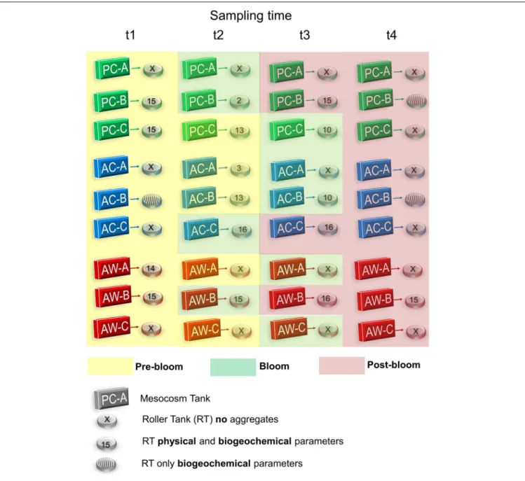
A controlled mesocosm experiment provided material for our aggregation experiments (Figure 1). The mesocosm experiment was conducted indoors at the Flax Pond Marine Laboratory of Stony Brook University during July 2011. Nine tanks (∼1 m3)
FIGURE 1 |Experimental setup for the mesocosm (cubes) and aggregation (cylinders) experiments. There were three treatments: present CO2-cooler (PC, 380 ppm and 16◦C) in green; acidified-cooler (AC, 750 ppm and 16◦C) in blue; and acidified-warmer (AW, 750 ppm and 20◦C) in red. Water was removed from each mesocosm four times (t1 to t4) during Pre-bloom (in yellow), Bloom (in green) and Post-bloom (in red) to start aggregation experiments. After 48 h, roller tanks that formed aggregates were video recorded. Not all roller tanks formed aggregates; the number inside the roller tanks represent the number of aggregates analyzed in the captured video, and roller tanks that did not form aggregates are marked with an “x”.
were filled simultaneously with seawater from Stony Brook Harbor, NY, United States, that was collected at approximately 3 m depth using a submersible pump; water was collected during the day at high tide several days after a large storm (Salinity 29).
The water was filtered through a 200-µm size mesh to remove large detritus and zooplankton before filling the tanks. Three treatments of variable CO2 and temperature where performed in triplicate: (1) acidified-cooler (AC, 750 ppm CO2, 16◦C), (2) acidified-warmer (AW, 750 ppm CO2, 20◦C), and (3) present CO2-cooler (PC, 390 ppm CO2, 16◦C). The triplicate mesocosms
were designated A, B, and C (e.g., AC-A, AC-B, AC-C) (Figure 1).
As a light source, pairs of fluorescent lights (F40T12, full spectrum) were suspended above each tank, providing a surface irradiance of 190µmol photons m−2s−1with a light: dark cycle of 14:10. Irradiance was set at the beginning the experiment with a LICOR Model LI-2100 light meter. All mesocosms were slowly stirred by mechanically-controlled paddles located in the middle of the mesocosm. The desired future CO2concentration (750 ppm) was achieved by initial addition of approximately 5 L of high-CO2 seawater (pH 4.8) previously filtered through
0.2 µm filters, rather than by bubbling with CO2, which risks formation of exopolymer particles. The pH corresponding to 750 ppm was calculated using the program CO2SYS (Lewis et al., 1998); total alkalinity (TA) was measured at the beginning of each experiment to calculate the pH corresponding to the desired CO2concentration (Supplementary Table S1). The pH was monitored once a day to determine the amount of high- CO2seawater to add (between 1 and 2 L every 24 h) to maintain the desired CO2 concentration. We added the high CO2 water and monitored the pH simultaneously until the target pH was achieved. The high CO2 water was added to the center of the mesocosm and was quickly homogenized (<10 min) with the help of the mechanically controlled paddles. Room temperature was held relatively constant at 20±1◦C; the tanks at 16◦C were cooled by circulating cold water (4◦C) through silicone tubes installed inside the tanks. We controlled the temperature gradient by adjusting the length of the silicon tube inside the mesocosm.
The cooling system and the amount of high CO2seawater needed daily to maintain the temperature and pH at desired values were determined during the 5 days of stabilization before sampling commenced.
The pH and temperature were measured at least once a day in the mesocosm tanks using YSI Pro 1030 waterproof handheld meters and standard DIN/NBS buffers (PL 4, PL 7, and PL 9) recalibrated using Tris-based reference material provided by A. Dickson (Nemzer and Dickson, 2005). TA was measured by titration (Gran, 1952) with 0.1N HCl using a Gilmont micrometer burette and an Orion model 370 pH meter. Salinity was measured with a hand-held refractometer when the mesocosm tanks were first filled.
Conditions during the mesocosm experiments are shown in the Supplementary Material and summarized here briefly.
Temperature and pH were monitored daily throughout the experiments (Supplementary Figure S1), and clearly show that the desired differences in pH and temperature were achieved. For acidified tanks, the target pH (7.7) corresponding to 750 ppm CO2 was calculated using the measured initial values of temperature (16.8±0.8 and 18.3◦C for AC and AW, respectively), and TA (1786.7 ± 46.2 and 1840.0 ± 40.0 µmol kg−1) (Supplementary Table S1). After 5 days of stabilization, the desired temperature and pH in the mesocosm tanks were achieved; PC: pH 8.1 ± 0.1 and 16.1±0.5◦C; AC: pH 7.79±0.10 and 16.2±0.4◦C, and AW:
pH 7.8 ±0.10 and 20.1± 0.4◦C (Supplementary Figure S1).
Nutrients were added on day five (final concentration: 20 µM nitrate, 20 µM silicate, and 1.5 µM phosphate) to initiate a phytoplankton bloom; the phytoplankton bloom started quickly 24 h after the nutrients were added as seen by the immediate increase in Chl a on day 7 (Supplementary Figure S2). The bloom was monitored for 21 days; during this period the mesocosm tanks were sampled six times, and four roller tank aggregation experiments were conducted to study aggregates at different stages of the phytoplankton bloom (days 10, 13, 16, and 19, Figure 1). The bloom stages were not reached at the same time in all mesocosms (Figure 2andSupplementary Table S2).
The “Bloom Peak” of each tank is defined as the sampling point when the Chl-a concentration was the highest; the sampling
points before the Bloom Peak are called “Pre-Bloom” and those after the Bloom Peak are called “Post-Bloom” (Supplementary Table S2).
Biological and Chemical Analyses
Nutrient samples were filtered through 0.2-µm syringe filters and stored in the refrigerator (4◦C) until analysis (no longer than 2 weeks). Measurements of nitrate, phosphate and silicate were made at the SoMAS Analytical Laboratory using a Lachat Instruments QuickChem FIA5000 autoanalyzer and the standard spectrophotometric methods described byParsons et al. (1984).
Detection limits were 0.3µM for nitrate, 0.2µM for phosphate, and 0.1µM for silicate.
The phytoplankton composition in each mesocosm was examined with a portable FlowCAM system (Fluid Imaging, Inc.). The FlowCAM enables measurement and imaging of microscopic particles in two dimensions using a regular microscope objective lens as the particles pass through a glass chamber in a continuous flow (Sieracki et al., 1998). The FlowCAM automatically counts, sizes, and obtains individual pictures of each particle. All the measurements in this study were made using the automatic imaging mode and an objective lens of 10X, leading to an overall magnification of 100X. A 300-µm- deep flow cell allowed measurement of particle size between 2 and 300µm. A sample volume of 0.5 mL was analyzed, with a flow rate between 0.1 and 0.4 mL min−1and a camera rate of 7.0 frames s−1. Between samples, the system was flushed with Milli- Q water for 5 to 10 min at a flow rate of 0.5 mL min−1, and a visual inspection of the flow cell was performed between samples to ensure cleanliness. During each run, samples were gently mixed with a small stirring bar to prevent particle sedimentation, and were pumped through the flow cell using a peristaltic pump.
Samples were diluted with 0.2µm filtered artificial seawater when needed. Results were analyzed using Visual Spreadsheet Software version 3.1.10 (Fluid Imaging, Inc.).
Total particulate carbon (TPC) and PN content were quantified at the SoMAS Analytical Laboratory using a Carlo Erba EA-1112 CNS analyzer (uncertainty ± 2% for C and ± 5% for N analysis). Duplicate samples of 20–50 mL were filtered onto combusted GF/F filters. PIC was not removed because preliminary analysis showed negligible differences in carbon between HCl-treated and non-treated samples. The mesocosm experiments were dominated by diatoms, with a minimal presence of calcifiers. Concentrations of chlorophyll a (Chl a) were determined using high-performance liquid chromatography (HPLC) (Mantoura and Llewellyn, 1983;
Bidigare et al., 1985), as a proxy for phytoplankton. Briefly, 20 to 50-mL samples were filtered onto combusted GF/F filters in duplicate and frozen until analysis. Pigments were extracted from filters and analyzed as described inSun et al. (1991). TEP and CSP were analyzed spectrophotometrically after staining with a solution of 0.02% AB (Alcian Blue 8X, Sigma Aldrich) at pH 2.5 and a solution of 0.04% CBB (Coomassie Brilliant Blue G-250, SERVA electrophoresis) at pH 7.4, according to Passow and Alldredge (1995a)andCisternas-Novoa et al. (2014), respectively. Blanks were prepared from Milli-Q water or 0.2-µm filtered seawater (FSW) for each set of samples. Concentrations
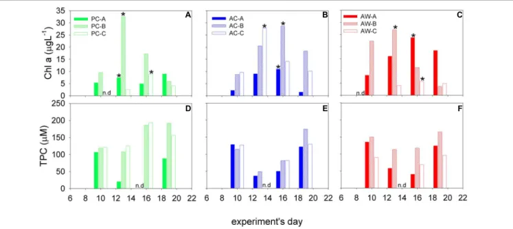
FIGURE 2 |Chl-a(A–C)and TPC(D–F)concentrations in the mesocosms at the time each roller tank aggregation experiment was started. Black star indicates the
“bloom peak” in each mesocosm. Triplicate mesocosms were run for each of the three treatments: present CO2-cooler (PC, green), acidified-cooler (AC, blue), and acidified-warmer (AW, red); n.d., no data.
of TEP are reported relative to a xanthan gum standard and expressed in micrograms of xanthan gum equivalents per liter (µg XG eq. L−1) afterPassow and Alldredge (1995a). For CSP measurements, stained filters were extracted and incubated as in Cisternas-Novoa et al. (2014). Concentrations of CSP are reported relative to a bovine serum albumin standard and expressed in micrograms of bovine serum albumin equivalents per liter (µg BSA eq. L−1).
Roller Tank Experiments (RTEs)
An aggregation experiment was conducted with water from the mesocosms during different stages of the phytoplankton bloom as described inFigure 1. One roller tank was filled for each of the nine mesocosms at four sampling times (a total of 36 roller tanks). Each 5-L roller tank (23-cm diameter) was filled with water sampled from the center of the mesocosm using a silicon tube, and then incubated on a roller table to promote aggregate formation (Shanks and Edmondson, 1989). No visible aggregates were observed in mesocosm water at the start of any of the aggregation experiments. Tanks were rotated at 0.8 rpm in the dark at room temperature. We visually monitored the appearance of aggregates, and sampled the roller tanks after 48 h. Before sampling, each rotating roller tank was filmed for 10 min using a video camera; single images, captured from these videos, were analyzed later to determine physical parameters of the aggregates as described below. Then, each roller tank was taken out the roller table, turned on its base, and the particles were allowed to settle to the bottom for 20 min. To determine the concentration of the particulate constituents (Chl a, TPC, PN, TEP, and CSP), we collected samples of two fractions from each roller tank: (a) surrounding seawater (SSW) and (b) aggregate “slurry” fraction (SL) that was a mixture of aggregates (AGG) and the inevitable
small amount of SSW collected with them. After removing the upper tank lid, SSW was carefully removed from the upper part of the tank with a piece of Tygon tubing by gravity into a 2- L Nalgene bottle. For the SL fraction, following Engel et al.
(2009a), visible aggregates (i.e.,>0.4 mm) that had sunk to the bottom of the roller tank during the 20-min settling period were carefully removed with the minimum amount of SSW using a 10- ml serological pipette and gentle suction. The volume of the SL was measured inside the pipette before transferring it to a 1-L Nalgene bottle. This process was repeated until all the aggregates were removed. The total volume of aggregate slurry was between 5 and 160 mL. Then, 300 mL of 0.2-µm FSW was added to the slurry and gently mixed to provide enough sample volume to split for all the analyses.
The SSW fraction volume was always larger than the AGG fraction volume in the slurry mixture; however particle concentration in the AGG fraction is in general 2 to 4 orders of magnitude larger than in the SSW fraction (Engel et al., 2002, 2009a). To determine the concentration of the particulate constituents, such as Chl a, TPC, PN, TEP, and CSP in the AGG fraction, concentrations in the SSW fraction were subtracted from those in the SL fraction following Engel et al. (2009a); in this way, CAGG, the concentration (µg L−1) of each constituent in the AGG fraction is reported per liter of roller tank water using the following equation:
CAGG= ASL+FSW
Vfiltered
∗ VSL+FSW
VSL
−CSSW,
where ASL+FSW is the mass (µg) of each constituent in the aggregate slurry (SL) plus the added FSW, Vfilteredis the volume (L) of SL plus added FSW filtered to determine each constituent,
VSL+FSW is the total volume (L) of SL plus the added FSW, VSL is the is the total volume (L) of the SL, and CSSW is the concentration (µg L−1) of each constituent in the SSW fraction.
Determination of Aggregate Size (ESD), Sinking Velocity (U), Excess Density ( 1ρ ), and Mass
Determination of sinking velocity and aggregate size using rolling tanks is non-invasive and does not require isolation or manipulation of the aggregates, making this method suitable to study fragile marine aggregates. Rolling tank studies do have issues related to the extrapolation and comparison of aggregates formed in a closed system versus those naturally occurred in the ocean (Engel and Schartau, 1999;Jackson, 2015). However, this approach is appropriate to investigate relative differences in sinking velocity under different treatments, such as the present study. There are several methods used to estimate sinking velocity using rolling tanks (Engel and Schartau, 1999;Ploug et al., 2010;
Jackson, 2015). In this study we measured sinking velocity and aggregate size using the two-point method proposed by Engel and Schartau (1999). This method is based on analysis of images captured from a video recording of the aggregates. Then, 1ρ was derived from the sinking velocity measurements (Engel and Schartau, 1999). This method was preferred for practical and technical considerations. At the time of our experiment this method had been successfully used in previous studies (Engel et al., 2009b; Biermann and Engel, 2010); moreover, it allows the determination of sinking velocity and size of aggregates even when they are smaller than 0.5 mm. The equivalent spherical diameter (ESD) of aggregates measured in this study ranged between 0.39 and 9.16 mm. The relatively small size of aggregates at the lower limit of the size range combined with technical issues like the presence of visible scratches in some of our roller tanks required that the magnification needed for the observation and imaging was, in most cases, too high to include the whole orbit of the cylinder tank, a requirement to use the method ofPloug et al.
(2010). To achieve accurate measurements, we chose to image only aggregates in the front of the roller tank, therefore ensuring that the aggregates were in focus.
The size of aggregates and their sinking velocity within the roller tanks were determined from pictures captured from the video recording of aggregates in the roller tank. After rotating for 48 h in the dark, tanks were recorded for 10 min with a Sony CCD-TRV338 Hi8 Handycam camcorder (3.2 megapixels).
Since the aggregates formed in each roller tank were different in number, size and compactness, the roller tanks were recorded at the optimal magnification, and the optical resolution of each video was calibrated individually. The observation window varied between 3.5 and 8.0 cm in width and between 2.3 and 5.3 cm in height, and was always located in the horizontal axis that intersected the center of the tank. Single pictures were captured from the video and analyzed as inEngel and Schartau (1999)and Engel et al. (2009b). Images were captured with the software “Free Video to JPG Converter” (DVD Video Soft Limited). Between 10 and 20 randomly-chosen aggregates from each roller tank
were analyzed (when there were less than 10 aggregates in the roller tank, the maximum possible number was analyzed). To ensure the accuracy of the calculation of the vertical velocity component of the fluid, we only analyzed aggregates in their circular trajectory i.e., the displacement in the horizontal plane was 5% or smaller than displacement in the vertical plane, for more details about the method to determine the sinking velocity of an aggregate inside a roller tank, please seeEngel and Schartau (1999). Aggregate parameters such as area, length of the major axis, length of the minor axis, the x-feret diameter and position in the x–y plane, were measured semi-automatically using public domain ImageJ software, and were used to estimate aggregate dimensions and settling velocity. The visible volume (V), ESD, and the area of the aggregates perpendicular to the fall direction were calculated. The aggregate sinking velocity (U) was determined from its apparent velocity, which can be estimated from the vertical displacement of the aggregate with time. The excess density of individual aggregates (1ρ) was calculated from their sinking velocity and size using the equation presented inIversen and Ploug (2010). Aggregate mass was determined by multiplying1ρ times the aggregate volume (V) and fitting the data to a power curve. The median U, ESD, and 1ρ of the measured aggregates were calculated for each roller tank or treatment at different stages of the phytoplankton bloom.
The median of those parameters was also compared to the biogeochemical particulate components of aggregates (TPC, PN, TEP, CSP, and Chla) that were measured on the bulk aggregate fraction as described above.
Statistical Analysis
The linear correlation between any two physical and biogeochemical characteristics of the aggregates was evaluated using the Spearman’s coefficient (r). Statistical significance was accepted for p < 0.05. Multivariate analyses of variance (MANOVA), based on aggregate sinking velocity and physical properties (ESD,mass, and1ρ), were used to evaluate whether these properties were significantly different in aggregates formed under different CO2 and temperature conditions. In addition, the influence of the treatments on each physical parameter (U, ESD, mass, and1ρ) of the aggregates was tested by Kruskal–
Wallis tests, followed by multiple comparison analyses for each parameter mean (ESD, U,1ρ, and mass) to determine whether the medians of those parameters were significantly different for any pair of treatments. Power law curves fit to the data were used to determine the relationship between aggregate physical properties (U andESD). Anr2 andp-value was calculated as a measure of goodness and significance, respectively, of the curve fit. All the calculations and statistical tests were run using MatLab R2014a.
RESULTS
Mesocosm Experiment and Starting Conditions for Aggregation Experiments
The Bloom intensity was variable and the Bloom Peak was reached at different times in each mesocosm (Figure 2A).
Diatoms dominated the phytoplankton community in all the mesocosms; qualitative analysis of FlowCAM data revealed that the phytoplankton blooms were mainly composed of small centric diatoms and larger chain-forming diatoms such as Nitzschia closterium, Ditylum brightwellii, Eucampia zodiacus, Leptocylindrussp., andPseudo-nitzschiasp.
Although the Bloom Peak was reached at different times in each mesocosm, we observed no measurable difference in the time, magnitude, or phytoplankton composition of the bloom that could be attributed to the acidification and/or temperature treatments. The concentration of the biogeochemical parameters (TPC, PN, Chl a, TEP, CSP, and nutrients) were also not significantly different among treatments (Supplementary Figures S2, S4, S5).
Particle concentrations measured in the mesocosm experiments were considered to be starting conditions for the aggregation experiments. Chl a varied between 1.5 and 33µL−1 (Figure 2) and the maximum concentrations were at t2 and t3. TPC concentrations ranged between 20 and 193µM, and were relatively higher during t1 and t4 in treatments AC and AW, but increased from t1 to t4 in treatment PC (Figure 2).
Highest concentrations of exopolymeric particles normalized to TPC were measured during the bloom peak and coincided with the Chl-amaximum (t2 and t3).
Aggregate Formation
No visible (>0.4 mm) particles were observed when the roller tanks were initially filled with seawater taken from the mesocosms at any stage of the phytoplankton bloom. Aggregates did not form in every roller tank experiment (RTE). Three roller tanks (t1 AC-B, t4 PC-B, and t4 AC-B) did form aggregates, but due to their small size and problems with the roller tanks, we only analyzed the concentration of the particulate constituents in the SL fraction and not the physical parameters (ESD and U; Figure 1). However, we did measure physical properties in aggregates that formed in seven roller tanks before the Bloom Peak, five during the Bloom Peak and six after the Bloom Peak (Supplementary Table S3). No aggregates formed in any of the PC-A and AW-C RTEs. There was no significant correlation between aggregate formation and the CO2/temperature treatment of the mesocosm tanks. Considering all treatments and bloom times, there was a correlation between aggregate formation (as the volume of aggregate slurry) in the RTE and the concentration of TPC (r = 0.36, p < 0.05), PN (r= 0.60,p<0.001), TEP (r= 0.49,p<0.01), and CSP (r= 0.60, p <0.0001) in the mesocosm at the starting time of the RTE.
The volume of aggregate slurry fraction collected in each roller tank and the number of aggregates analyzed for determination of physical properties are shown inSupplementary Table S3.
Aggregate Composition
We did not observe statistically significant differences in aggregate composition among different CO2 or temperature treatments. However, the chemical composition of aggregates changed during the course of the experiment, and those changes were not equally evident or statistically significant in all treatments. All aggregates were enriched in exopolymer
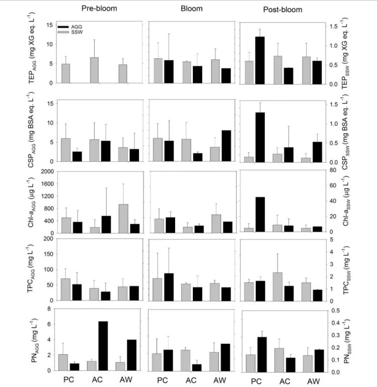
particles (TEP and CSP), TPC, PN, and Chl a relative to the SSW and independently of the treatment or bloom time (Figure 3). Exopolymer particle contents of aggregates increased with bloom stage in the PC (TEP: r = 0.78, p < 0.05 and CSP: r = 0.86, p < 0.05) and AW (TEP: r = 0.75, p = 0.13) treatments. No significant difference in the Chl a, TPC, or PN content of the aggregates was observed at different bloom stages.
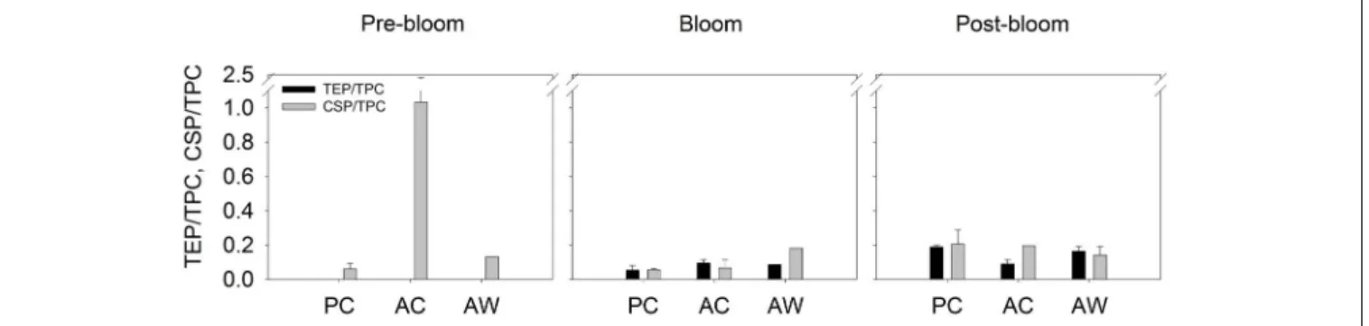
Exopolymer particles normalized to TPC concentration showed that TEP/TPC and CSP/TPC ratios appeared to be particularly higher in aggregates formed in AC treatment during Pre-Bloom (Figure 4), but those differences were not statistically significant.
If we consider the composition of all aggregate fractions together, independent of treatment or bloom time, there was a positive correlation between TEP and CSP content (r= 0.62, p<0.05, Supplementary Table S4). The concentrations of TEP and CSP increased with bloom stage (r = 0.60,p <0.05, and r = 0.63, p<0.01, respectively), and CSP was positively correlated with TPC (r= 0.80,p<0.001) and PN (r= 0.57,p<0.01).
Aggregate Size (ESD), Sinking Velocity (U), Excess Density ( 1ρ ), and Mass
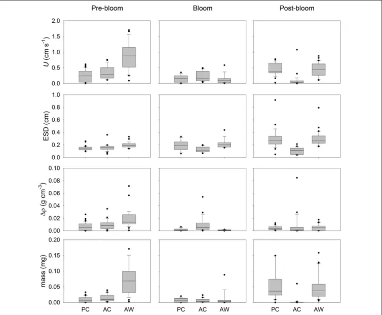
Considering all the aggregates formed in the four aggregation experiments together, independently of treatment, we observed that the ESD, U, and 1ρ changed throughout the bloom development. The ESD of aggregates formed in roller tanks at different bloom stages ranged between 0.04 and 0.92 cm (Figure 5). Smaller aggregates (0.06 to 0.18 cm) were observed during Pre-Bloom (median: 0.16 cm) and Bloom Peak (median:
0.17 cm); after the Bloom Peak the maximum ESD of aggregates in each tank was larger (median: 0.34 cm). Sinking velocity, U, ranged between 0 and 1.7 cm s−1 (Figure 5) and opposite to what might be expected from aggregate size, U measured before the bloom peak was faster (median: 0.37 cm s−1) than during the bloom (median: 0.15 cm s−1) and after the bloom peak (median: 0.34 cm s−1). 1ρ of aggregates, calculated from U (Figure 5), ranged over four orders of magnitude (from 5×10⁻⁶ to 8 × 10⁻² g cm−3) and did not significantly changed with bloom time if we consider all treatments together, the median 1ρ was 8.5×10⁻³ g cm−3 during Pre-Bloom, 2.1 × 10⁻³ g cm−3during Bloom Peak, and 3.1×10⁻³g cm−3during Post- Bloom. The calculated aggregate mass (Figure 5) varied between 1×10⁻⁵and 2×10⁻¹mg without a clear relationship with the bloom stage.
An initial multivariate analyses of variance (MANOVA, data not shown), comparing aggregate physical properties (ESD, U, 1ρand mass), showed that aggregates formed from mesocosm seawater subjected to different CO2and temperature conditions, were significantly different from each other. During Pre-Bloom, the physical properties of the aggregates formed in PC and AC treatments overlapped, but properties of aggregates from AW treatments were different. During and after the Bloom Peak, properties of aggregates formed in the AC treatment were significantly different from those of aggregates formed in PC and AW treatments. Since physical properties of aggregates formed in different treatments were significantly different from each other, aggregates from the same treatment and bloom period
FIGURE 3 |TEP (mg XG eq. L−1), CSP (mg BSA eq. L−1), Chl-a(mg L−1), TPC (mg L−1), and PN (mg L−1) contents of the aggregate fraction (AGG, gray) and surrounding seawater fraction (SSW, white) formed during RTEs. The bars represent the average of all the roller tanks that formed aggregates in each treatment and bloom period. For Pre-bloom: PC (n= 3RT), AC (n= 4 RT), and AW (n= 2RT); and for Post-bloom PC (n= 2 RT), AC (n= 2 RT), and AW (n= 2 RT).
were analyzed together and the three treatments were compared (Figure 5andTable 1).
The Kruskal–Wallis test with posterior mean rank multiple comparisons revealed specifically in which cases the analyzed parameters (ESD, U,1ρ, and mass) were significantly different between treatments (Table 1). The median U, ESD, 1ρ, and
mass of the aggregates formed in Pre- Bloom in AW treatment were significantly larger than aggregates formed in PC and AC treatments (Table 1). During the Bloom Peak, the U of aggregates formed in AW was not significantly different than in the other two treatments. The median U, 1ρ, and mass of aggregates formed in AC were larger than in aggregates formed in PC,
FIGURE 4 |Content of TEP (mg XG eq. L−1) and CSP (mg BSA eq. L−1) normalized by the amount of TPC in the aggregate fraction of each treatment and sampling time. Black bars represent the TEP/TPC ratio and gray bars represent CSP/TPC. Bars show the average of all the roller tanks that formed aggregates in each treatment and bloom period. For Pre-bloom: PC (n= 3RT), AC (n= 4 RT), and AW (n= 2RT); and for Post-bloom PC (n= 2 RT), AC (n= 2 RT), and AW (n= 2 RT).
however the median ESD of aggregates formed in AC was smaller than in PC. There were no significant differences in ESD,1ρ, and mass of aggregates formed in PC and AW. During Post-Bloom, the U, ESD, and mass of aggregates formed in AC were all smaller than in aggregates formed in PC and AW (Figure 5andTable 1).
There were not significant differences between aggregates formed in AW and PC.
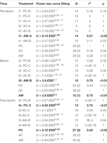
The relationships between U and ESD of the aggregates during the different stages of the bloom were determined using power law curves fit to the data from each roller tank.
However, with only few exceptions (Table 2), there was no significant relationship between those parameters. There was a significant positive relation between U and ESD in roller tank AW-A t1 before the Bloom Peak, roller tank AW-B t2 during the Bloom Peak, and roller tank PC-C t4 after the Bloom Peak.
DISCUSSION
Starting Conditions for the Aggregate Experiments
The primary goal of the mesocosm experiment was to provide material to investigate aggregation processes. The sinking of phytoplankton-rich aggregates is the major export mechanism by which photosynthetically fixed carbon reaches the deep ocean (Alldredge and Jackson, 1995; Buesseler, 1998; Turner, 2015). However, information is scarce about the direct effect of acidification and warming on aggregation rates and sinking velocities (Seebah et al., 2014), and most existing studies focus only on effects of temperature (Piontek et al., 2009; Iversen and Ploug, 2013) or of acidification on calcifying organisms (Biermann and Engel, 2010). In our RTEs, we aimed to investigate how warming and acidification together will affect future aggregation and thus export processes during the different stages of a natural phytoplankton bloom dominated by diatoms.
Roller tank aggregation experiments were performed during Pre-Bloom, Bloom Peak, and Post-Bloom periods to compare a wide range of Chl-a and nutrient concentrations. Chl-a concentrations at the Bloom Peak were relatively high compared with environmental values due to the addition of nutrients to
induce a phytoplankton bloom. Concentrations of particulate organic matter (Chl a, TPC, and exopolymeric particles) measured in the mesocosms before RTEs were used as the initial concentration of material available for aggregate formation. In general, during Pre- and Post-Bloom, TPC was higher and the ratio TEP/TPC and CSP/TPC were lower relative to the Bloom- Peak (Figure 2).
Visible (>0.4 mm) aggregates did not form in every roller tank aggregation experiment. Coagulation theory indicates that aggregate formation is controlled by the abundance of particles that could potentially aggregate, their size and stickiness, i.e., the probability that those particles stick together after collision (Jackson, 1990; Kiørboe et al., 1990). The magnitude of the bloom in each mesocosm tank is one indicator of the abundance of particles available to form aggregates. Thus, the initial concentration of Chl-a reflects the number of cells and thus higher Chl-a would cause higher aggregate formation.
For instance, AW-C and PC-A mesocosms had low Chl-a and exopolymer particle concentrations and did not form aggregates; PC-C also had relatively low Chl-a concentration (<10 µg L−1), but a comparatively higher concentration of exopolymer particles, and did form aggregates (except at the last time point). Intuitively, we tend to think that a larger bloom (with higher Chl-aconcentrations) would result in higher cell concentrations and higher production of exopolymer particles and thus enhanced aggregate formation.
TEP concentration is another possible indicator of the potential to form aggregates. TEP have been shown to enhance aggregation in two different ways: first increasing the concentration of particles in the water and thus the probability of collision, and second, increasing particle stickiness by up to two orders of magnitude thus increasing the probability that two particles will stick together after collision (Logan et al., 1995;
Passow and Alldredge, 1995b;Engel, 2000;Passow, 2002). TEP concentration has been positively related to aggregate formation in mesocosm experiments with coastal phytoplankton (Passow and Alldredge, 1995b; Engel et al., 2014) and a non-axenic culture ofThalassiosira weissflogii(Seebah et al., 2014). However, exopolymer particles such as TEP and CSP can have different effects on aggregate formation depending on the dominant species. For example, significant amounts of TEP and CSP were
FIGURE 5 |Sinking velocity and physical properties of aggregates formed in RTEs conducted at different bloom periods. The box plots include all the individually-measured aggregates (>0.4 mm) from the different roller tanks (RT) in each treatment. For Pre-Bloom, PC included 29 aggregates from two RT, AC included 29 aggregates from three RT, and AW included 29 aggregates from two RT. For Bloom Peak, PC included 25 aggregates from two RT, AC included 26 aggregates from two RT, and AW included 15 aggregates from one RT. For Post-Bloom, PC included 27 aggregates from two RT, AC included 26 aggregates from two RT, and AW included 30 aggregates from two RT. The boundaries of the box indicate the 25thand the 75thpercentile, the black line within the box is the median. Error bars indicate the 90thand 10thpercentiles, and black dots are the outlying points.
not observed in aggregates formed from pure cultures ofNavicula sp. (Grossart et al., 2006), while Prieto et al. (2002) showed that CSP had a less important role than TEP in aggregation events studied in mesocosms, However, the Prieto et al. (2002) study looked at the relation between CSP and aggregation during the aggregate maximum, which may coincide with lower CSP concentration (Cisternas-Novoa et al., 2015).
The type of cell may also influence aggregation; for example, not all diatom types make the same contribution to aggregate formation and sinking velocity (Laurenceau-Cornec et al., 2015).
In this experiment, we did not detect any qualitative differences in diatom composition that were related to the temperature and acidification treatments. In most mesocosms, chain-forming
and small centric diatoms dominated the phytoplankton bloom.
Exceptions were mesocosm PC-A and AC-A (Supplementary Figure S6), in which small centric diatoms were dominant; few or no aggregates formed in water from those mesocosms. However, aggregation experiments with water from AW-C also formed no aggregates, despite the fact that both chain-forming and small centric diatoms were present, although the bloom was relatively small. Thus, differences in diatom type alone could not explain the presence or absence of aggregates in the RTEs.
In our aggregation experiments, there was a correlation between aggregate formation in the RTEs and the initial concentration of TPC, PN, TEP, and CSP at the beginning of the RTE. During this study we did not investigate the role of bSi as
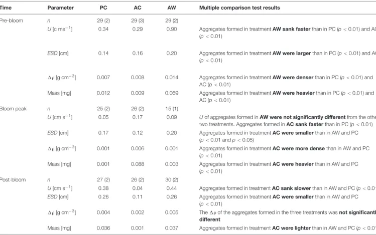
TABLE 1 |Median and results of the Kruskal–Wallis test with posterior multiple comparisons analysis for the RTEs.
Time Parameter PC AC AW Multiple comparison test results
Pre-bloom n 29 (2) 29 (3) 29 (2)
U[c ms−1] 0.34 0.29 0.90 Aggregates formed in treatmentAW sank fasterthan in PC (p<0.01) and AC (p<0.01)
ESD[cm] 0.14 0.16 0.20 Aggregates formed in treatmentAW were largerthan in PC (p<0.01) and AC (p<0.01)
1ρ[g cm−3] 0.007 0.008 0.014 Aggregates formed in treatmentAW were denserthan in PC (p<0.01) and AC (p<0.01)
Mass [mg] 0.012 0.009 0.069 Aggregates formed in treatmentAW were heavierthan in PC (p<0.01) and AC (p<0.01)
Bloom peak n 25 (2) 26 (2) 15 (1)
U[cm s−1] 0.05 0.17 0.09 Uof aggregates formed inAW were not significantly differentfrom the other two treatments. Aggregates formed inAC sank fasterthan in PC (p<0.01) ESD[cm] 0.17 0.12 0.20 Aggregates formed in treatmentAC were smallerthan in AW and PC
(p<0.01 andp<0.05)
1ρ[g cm−3] 0.001 0.006 0.001 Aggregates formed in treatmentAC were more densethan in AW and PC (p<0.01)
Mass [mg] 0.001 0.088 0.003 Aggregates formed in treatmentAC were heavierthan in AW and PC (p<0.01)
Post-bloom n 27 (2) 26 (2) 30 (2)
U[cm s−1] 0.38 0.04 0.44 Aggregates formed in treatmentAC sank slowerthan in AW and PC (p<0.01) ESD[cm] 0.26 0.11 0.26 Aggregates formed in treatmentAC were smallerthan in AW and PC
(p<0.01)
1ρ[g cm−3] 0.004 0.002 0.005 The1ρof the aggregates formed in the three treatments wasnot significantly different
Mass [mg] 0.036 0.001 0.037 Aggregates formed in treatmentAC were lighterthan in AW and PC (p<0.01)
“n” indicates the number of aggregates analyzed, and the number between parentheses indicates how many roller tanks they came from. Parameters compared were excess density (1ρ, g cm−3) and mass (mg) of the aggregates calculated from measured values of sinking velocity (U, cm s−1), and equivalent spherical diameter (ESD, cm).
a ballast; further studies should incorporate this measurement to obtain a complete, and ideally, a more robust idea of how different particulate components interact to form aggregates. Our results do show that the abundances of cells, TEP, and CSP may be important for aggregate formation, but they also suggest that the ratio of cells to exopolymer particles could be a determinant in aggregate formation.
Sinking Velocity (U) and Aggregate Size (ESD) Determination in Roller Tank Using Image Analysis
Obtaining accurate measurements of sinking velocity and physical properties of aggregates and relating them to compositional changes is a major challenge, but one that is critical to determining how climate change will affect aggregate properties and carbon export in the future ocean. The size and sinking velocity of aggregates measured in this study (43.2–380.1 m d−1) were comparable to values reported by Laurenceau-Cornec et al. (2015), between 13 and 260 m d−1 in RTEs with natural phytoplankton, and byIversen and Ploug (2010) between 113 and 246 m d−1 in RTEs with Emiliania huxleyi and Skeletonema costatum. During the Pre-bloom in treatment AW, we measured higher sinking velocities (median:
777.6 m d−1); this relatively high value was in the range reported byEngel and Schartau (1999), between 544.3 and 622.08 m d−1 in RTEs withNitzschia closterium.
Relation Between Chemical Composition and Physical Properties of Aggregates
We observed significant relationships between chemical composition and physical properties of aggregates; however, it is important to keep in mind that chemical and physical parameters were measured differently. The chemical composition of aggregates was measured in the aggregate slurry fraction, and the actual concentration of the particulate components was calculated after subtracting the concentration in the SSW (see section “Materials and Methods” for details). U andESD were measured in 10 to 20 randomly chosen aggregates, and 1ρ and mass were calculated from U and ESD. Thus, only relationships between the median of the directly measured physical parameters (UandESD) and the chemical composition of aggregates will be discussed. Considering each bloom stage separately, we found a weak correlation between TEP andESD (r= 0.78,p= 0.07) during Pre-Bloom and between CSP andESD (r = 0.82, p = 0.08) during Bloom-Peak. During Post-Bloom, however, there was a significant correlation between TEP: TPC ratio and ESD(r= 0.94,p<0.005). When we compare all the
TABLE 2 |Relationship between sinking velocity (U, cm s−1) and size as equivalent spherical diameter (ESD, cm) in each roller tank and bloom period.
Time Treatment Power law curve fitting N r2 p
Pre-bloom t1- PC-B U= 3.04ESD1.1 14 0.16 0.16
t1- PC-C U= 0.32ESD5.5E−17 15 0 1
t1- AC-A U= 0.47ESD3.3E−17 11 0 1
t2- AC-A U= 0.53ESD4.8E−17 5 0 1
t2- AC-B U= 0.19ESD1.3 E−13 13 0 1
t1- AW-A U= 8.15ESD1.62 14 0.37 <0.05
t1- AW-B U= 2.47ESD0.46 15 0.11 0.23
PC U= 0.25ESD5.8E−18 29 (2) – 1
AC U= 0.59ESD0.26 29 (3) 0.18 0.34
AW U= 2.73ESD0.69 29 (2) 0.29 0.13
Bloom t2- PC-B U= 0.061ESD0.43 15 0.08 0.30
t3- PC-C U= 0.20ESD1.6E−16 10 −4.4E-15 1
t2- AC-C U= 0.80ESD0.43 16 0.06 0.35
t3- AC-B U= 1.0 ESD1.1E−16 10 −2.2E-16 1 t2- AW-B U= 3.9ESD2.3 15 0.75 <0.01
PC U= 0.42 ESD0.36 25 (2) 0.43 0.12
AC U= 0.23 ESD9.9E−8 26 (2) – 1
AW U= 3.9 ESD2.3 15 (1) 0.75 <0.01 Post-bloom t3- PC-B U= 0.57ESD2.3E−17 14 −2.2E-17 1
t4- PC-C U= 0.83ESD0.63 13 0.75 <0.01
t3-AC-C U= 3.7ESD1.8 16 0.04 0.45
t4-AC-C U= 0.84ESD8.6E−17 10 −2.2E-16 1
t3-AW-B U= 0.54ESD0.03 15 5E-4 0.94
t4-AW-B U= 0.35ESD6.9E−17 15 −2.2E-16 1 PC U = 0.72 ESD0.34 27 (2) 0.45 <0.05
AC U = 0.06 ESD1.4E−16 26 (2) – 1
AW U = 0.44 ESD3.7E−17 30 (2) – 1
To show the fit of the power law curve, the total number of aggregates analyzed in each roller tank (n), r2and the p-value (p) are shown. Significant relationships (<0.05) are shown in bold.
treatments and blooms stages, the median ESD of aggregates was positively related to their TEP (r = 0.76, p < 0.005) and CSP (r = 0.74,p<0.005) contents (Supplementary Table S5).
Previous studies had shown that TEP are important in promoting the formation of larger aggregates as their stickiness enhances the coagulation of particles (Passow, 2002). The role of CSP in coagulation and aggregate formation still needs to be further investigated; diatom aggregates are depleted in CSP relative to TEP, while CSP seems to be an important component of cyanobacteria aggregates (Cisternas-Novoa et al., 2015). In our experiment, particle size was positively correlated with both TEP and CSP. However, this strong correlation between exopolymer particle content and ESD did not translate into a significant relationship between aggregate size (ESD) and U (Table 2). This discrepancy between aggregate size and U has been described before (Stemmann et al., 2004). Previous studies have shown that size influences U in specific cases, for instance, when aggregates are formed from homogeneous particles (Iversen and Ploug, 2010), or are highly compact (Laurenceau-Cornec et al., 2015). However, with increasing porosity (Iversen and Ploug, 2010) and TEP content (Engel and Schartau, 1999), the relationship between size andU becomes
weaker. TEP are less dense than seawater (Azetsu-Scott and Passow, 2004), which may explain why higher TEP content may decrease the U of aggregates (Engel and Schartau, 1999;
Mari et al., 2017). Our results (Table 2) agree with these previous findings that ESD is not always a good predictor of U for aggregates formed from natural plankton communities dominated by diatoms, and showed that an increment in size due to a higher content of exopolymer particles does not directly lead to higherU.
Particle size, density, and porosity have been proposed as the factors that control Uof aggregates (De La Rocha and Passow, 2007); this implies that chemical composition of the particles forming the aggregate has an indirect role determining theUof the aggregate. During this study we found a direct correlation between aggregate size and exopolymer particle content, but not between the chemical composition of aggregates andU.
Previous studies have shown that the TEP- U relationship is not straightforward (Seebah et al., 2014). On one hand, TEP content may decrease sinking velocity by adding low-density mass to an aggregate (Azetsu-Scott and Passow, 2004; Mari et al., 2017). On the other hand, TEP content may enhance sinking velocity by enhancing the formation of large, particle- loaded, and fast-sinking aggregates. TEP could also reduce the porosity of aggregates by filling pore spaces (Ploug et al., 2002);
this process may alter the U versus size relationship. In this study, the phytoplankton community was dominated by diatoms cells, which are denser than TEP. Solid matter density of large aggregates formed from a diatom culture ranges from 1.26 to 1.36 g cm−3 (Azetsu-Scott and Johnson, 1992), while the calculated density of TEP ranges from 0.70 to 0.84 g cm−3 (Azetsu-Scott and Passow, 2004). Therefore, if cells are embedded in a large TEP matrix, the more loaded with cells the matrix is, the denser the aggregate would be.Engel and Schartau (1999) previously showed that the higher the TEP content relative to cell volume concentration, the lower the value of fractal dimension (D3) andU. Our results showing that there is no direct correlation between exopolymer particle content and U agree with those of Laurenceau-Cornec et al. (2015); they studied the chemical composition and U of individual aggregates formed in roller tanks from natural seawater collected in the Kerguelen Plateau and suggested that chemical composition has no direct influence on aggregateU. Moreover, our findings of a correlation between exopolymer particles and size show the need for further parallel measurements on chemical composition and physical properties of aggregates.
Effect of Temperature and CO
2on Biochemical Composition and Physical Properties of Aggregates
In the aggregation experiment presented here, we did not detect a clear effect of temperature and CO2level on the biogeochemical composition of the aggregates, except in one case, the TEP and CSP content normalized to TPC of aggregates formed in AC treatment during Pre-bloom. A previous study showed that aggregates formed under high temperature (8.5 versus 2.5◦C) at the end of the bloom were enriched in POC, PN,
and POP (Piontek et al., 2009). Our results, however, are not directly comparable to the Piontek et al. (2009) study since the temperature range was different (16.5 to 20.5◦C), and the mesocosms at warmer temperature were also exposed to elevated CO2levels.
Although we did not detect changes in aggregate composition that could be attributed to the temperature or CO2 treatments, changes in aggregate composition did occur over the course of the phytoplankton bloom. TEP and CSP content in the aggregate fraction formed at present CO2and cooler temperature, and at elevated temperature and higher CO2, increased gradually from Pre-Bloom to Post-Bloom; this trend is not as clear at higher CO2 and cooler temperature. The content of TEP and CSP relative to TPC in the roller tank aggregates was also relatively higher during the Pre- and Post-Bloom than during the Bloom Peak (Figure 4). During Pre and Post-Bloom, the concentration of TEP and CSP relative to TPC was also high in the mesocosm. Thus, the higher concentration of TEP and CSP in the mesocosm water at the start of the roller tank aggregation experiment translated into elevated TEP and CSP content in the aggregate fraction.
This observation may suggest that a significant fraction of the TEP and CSP produced in the mesocosm was later incorporated in the aggregates, supporting the idea that TEP and CSP act as an “organic glue” enhancing aggregate formation (Engel, 2000;
Passow, 2002). The Chl-a and TPC content of the aggregate fraction, on the other hand, did not show a significant trend with the bloom stage.
Physical properties of the aggregates formed in the roller tanks were different under different CO2and temperature levels.
Aggregates varied significantly in size (measured as equivalent spherical diameter, ESD) and sinking velocity (U, Table 1).
Before the Bloom Peak, aggregates formed in acidified and warmer conditions were larger and sank faster than aggregates formed under cooler temperature, independent of the CO2level of the treatment. This suggests that the warmer temperature combined with the higher CO2 level had a synergistic effect on aggregate size and that temperature had a larger effect than CO2 level on aggregate sinking velocity. Previous mesocosm studies have suggested that the effect of warming is more important than acidification for a Baltic Sea phytoplankton community (Paul et al., 2015), and showed no measurable synergistic, but antagonist, effect of warming and acidification on phytoplankton biomass, Chl a and POC (Sommer et al., 2015; Paul et al., 2016). However, these studies did not investigate the direct effect on aggregates, Paul et al. (2015) found that the elevated temperature may have impacted phytoplankton growth before the bloom, leading to an earlier bloom peak, and enhancing the grazing pressure that controls the phytoplankton biomass. In our study, aggregates formed under warmer, acidified conditions had relatively higher contents of Chladuring Pre-bloom (Figure 3).
This agrees with the finding that the highest TEP/TPC and CSP/TPC ratio measured during this study was in aggregates formed under acidified but present temperature conditions during Pre-Bloom. These results suggest that under higher CO2 conditions at present temperature, the fraction of TEP and CSP relative to the TPC content of aggregates formed during Pre- Bloom in a diatom-dominated system could increase, causing
the formation of relatively large, but slowly sinking aggregates.
As mentioned earlier, higher TEP content might have decreased the U of aggregates (Engel and Schartau, 1999; Mari et al., 2017) since TEP are less dense than seawater (Azetsu-Scott and Passow, 2004). However, under higher CO2conditions combined with warming, the Pre-Bloom fraction of exopolymeric particles relative to TPC was not as high, suggesting that in a future warmer, more acidic ocean, large and fast sinking aggregates might be more abundant. One factor we need to consider is that we do not know the amount of bSi content (ballast material) in the aggregate fraction. Although TEP and CSP may decrease theU of aggregates, the1ρ of the aggregates does not depend only on TEP and CSP content but also on bSi content. If the stickiness of particles had decreased with bloom time (Dam and Drapeau, 1995), we could expect that the TEP and the bSi content of aggregates were closely related during the Pre-Bloom. This could explain why the highestU and the highest TEP and CSP content relative to TPC in treatment AC was during Pre-Bloom rather than Bloom peak and Post-Bloom. However, this was not observed in the other two treatments and since we do not have direct bSi measurements, this point is merely speculative.
During the Bloom Peak and Post- Bloom, physical properties of aggregates that formed at the same temperature but at different CO2levels were significantly different from each other (Table 1).
During the Bloom Peak, in general, aggregateUwas slower than during Pre- and Post-Bloom, except for aggregates formed under acidified conditions and ambient temperature that were relatively faster and smaller than aggregates formed under present CO2 levels and ambient temperature or under more acidified and warmer conditions. On the other hand, during Post-Bloom, aggregates that formed under acidified and ambient temperature conditions were smaller and sank more slowly (Table 1). The Post-Bloom situation in our experiment may be considered analogous to the culmination of a natural phytoplankton bloom.
In natural diatom-dominated phytoplankton blooms, senescent cells aggregate and sink at the culmination of the bloom (Logan et al., 1995; Thornton, 2002). Our results showed that under higher CO2 levels (without temperature change) conditions, slowly sinking aggregates would result in less POC export during Post-Bloom since aggregates that sink slower spend more time in the water column and have more time to decay. However, U of aggregates formed under acidified and warmer ocean conditions was not significantly different than aggregates formed under present conditions of CO2and temperature, this suggests that the negative effect of elevated CO2 onU could have been counteracted, and thus not detectable, by an opposite effect of warming.
Our study provides the first direct observations of the effect of temperature and acidification on aggregate sinking velocity and biogeochemical properties, highlighting the importance of directly investigating effects on aggregates instead of indirectly assuming them from effects on phytoplankton. The fact that we measure significant differences due to acidification and warming in physical properties but no in the chemical composition of aggregates could in part been explained by the different sampling strategy and resolution of those two types of parameters. To ensure to have enough material to characterize the chemical