In ﬂ uence of plankton community structure on the sinking velocity of marine aggregates

(1)

In ﬂ uence of plankton community structure on the sinking velocity of marine aggregates

L. T. Bach¹, T. Boxhammer¹, A. Larsen², N. Hildebrandt³, K. G. Schulz^1,4, and U. Riebesell¹

1GEOMAR Helmholtz Centre for Ocean Research Kiel, Kiel, Germany,²Hjort Centre for Marine Ecosystem Dynamics, Uni Research Environment, Bergen, Norway,³Alfred Wegener Institute Helmholtz Centre for Polar and Marine Research, Bremerhaven, Germany,⁴Centre for Coastal Biogeochemistry, Southern Cross University, East Lismore, New South Wales, Australia

Abstract

About 50 Gt of carbon isﬁxed photosynthetically by surface ocean phytoplankton communities every year. Part of this organic matter is reprocessed within the plankton community to form aggregates which eventually sink and export carbon into the deep ocean. The fraction of organic matter leaving the surface ocean is partly dependent on aggregate sinking velocity which accelerates with increasing aggregate size and density, where the latter is controlled by ballast load and aggregate porosity. In May 2011, we moored nine 25 m deep mesocosms in a Norwegian fjord to assess on a daily basis how plankton community structure affects material properties and sinking velocities of aggregates (Ø 80–400μm) collected in the mesocosms’sediment traps. We noted that sinking velocity was not necessarily accelerated by opal ballast during diatom blooms, which could be due to relatively high porosity of these rather fresh aggregates.

Furthermore, estimated aggregate porosity (P_estimated) decreased as the picoautotroph (0.2–2μm) fraction of the phytoplankton biomass increased. Thus, picoautotroph-dominated communities may be indicative for food webs promoting a high degree of aggregate repackaging with potential for accelerated sinking. Blooms of the coccolithophoreEmiliania huxleyirevealed that cell concentrations of ~1500 cells/mL accelerate sinking by about 35–40%, which we estimate (by one-dimensional modeling) to elevate organic matter transfer efﬁciency through the mesopelagic from 14 to 24%. Our results indicate that sinking velocities are inﬂuenced by the complex interplay between the availability of ballast minerals and aggregate packaging;

both of which are controlled by plankton community structure.

1. Introduction

Phytoplanktonﬁxes approximately 50 Gt of carbon in the euphotic zone of the oceans every year [Longhurst et al., 1995;Field et al., 1998]. Most of this organic carbon is remineralized in the surface ocean. However, 5–12 Gt C escape remineralization and are exported out of the surface (100 m), either as dissolved organic carbon (DOC) trapped in downwelling water currents, as particulate organic carbon (POC) sinking due to gravity, or transported downward by vertically migrating zooplankton [Hansell and Carlson, 2001;Turner, 2002;Honjo et al., 2008;Steinberg et al., 2008;Henson et al., 2011;Siegel et al., 2014]. A large fraction of the POC and DOC is biologically remineralized during its descent through subsurface water and released as dissolved inorganic carbon (DIC). That way, DIC is transported from surface to depth against a concentration gradient in a series of biologically mediated processes—the reason why this has been termed the biological pump [Volk and Hoffert, 1985]. A shutdown of the biological pump would lead to a signiﬁcant accumulation of DIC in the surface ocean paralleled by a roughly 60–70% increase of current atmospheric CO₂concentrations within a 1000 year equilibration time [Maier-Reimer et al., 1996]. This highlights the outstanding impor- tance of the biological pump for the global carbon cycle and climate.

The fraction of surface-originating POC that reaches the deep ocean depends on the balance between particle remineralization rates and sinking velocities. A fast-sinking particle made of relatively refractory POC will experience little remineralization during its descent from the euphotic zone (~0–200 m) through the mesopelagic (200–1000 m) into the deep ocean (below 1000 m). Conversely, a slowly sinking particle made of labile and easily disintegrating POC would never reach that far. Remineralization rates are controlled by bacterial activity and mesozooplankton feeding as well as particle fragmentation rates [Kiørboe, 2001;

Giering et al., 2014]. Sinking velocity is determined by the viscosity of seawater, particle size, shape, and excess density [Stokes, 1850;McNown and Malaika, 1950;Smayda, 1970], where the latter depends primarily on porosity of the particle and the amount of ballast mineral attached to it [Alldredge and Gotschalk, 1988].

Global Biogeochemical Cycles

RESEARCH ARTICLE

10.1002/2016GB005372

Key Points:

•Aggregate sinking speeds are controlled by processes in the plankton community

•Plankton communities can affect sinking speed by altering aggregate porosity and ballasting

•Emiliania huxleyiblooms of 1500 cells/mL increase organic matter transfer efﬁciency from 14 to 24%

Supporting Information:

•Supporting Information

Correspondence to:

L. T. Bach, lbach@geomar.de

Citation:

Bach, L. T., T. Boxhammer, A. Larsen, N. Hildebrandt, K. G. Schulz, and U. Riebesell (2016), Inﬂuence of plankton community structure on the sinking velocity of marine aggregates, Global Biogeochem. Cycles,30, doi:10.1002/2016GB005372.

Received 5 JAN 2016 Accepted 6 JUL 2016

Accepted article online 9 JUL 2016

(2)

Opal, CaCO₃, and lithogenic minerals are ballast materials formed in or deposited onto the oceans’surface layer. Opal is formed by diatoms, silicoﬂagellates, and radiolarians, while CaCO₃is mainly formed by cocco- lithophores, calcifying dinoﬂagellates, foraminifera, and pteropods. Lithogenic minerals are usually of terrige- nous origin and transported into the oceans via dust events or river input. Ballast minerals are important components in particle export as they may slow down remineralization of associated POC [Hedges and Oades, 1997] and increase particle excess density, thereby accelerating sinking velocity [e.g.,Passow and De La Rocha, 2006;Honjo et al., 2008;Ploug et al., 2008]. These mechanisms were used to explain the ballast ratio hypothesis [Armstrong et al., 2009], which originates from the observation that globally averaged POC:

ballast mineral ratios are high and variable in the euphotic zone but converge to relatively narrow and stable values in the deep [Armstrong et al., 2002]. The ballast ratio hypothesis suggests that ballast minerals, in particular relatively dense CaCO₃, strongly support deep ocean POC sequestration since most organic material reaching below 2000 m is associated with them [Francois et al., 2002;Klaas and Archer, 2002].

Recently, however, the ballast ratio hypothesis has been called into question.Passow and De La Rocha [2006] andBoyd and Trull[2007] noted that globally averaged correlations between ballast materials and POC may not be found on regional scales or along the course of an entire seasonal cycle. This concern was confirmed by the analysis ofWilson et al. [2012] andLe Moigne et al. [2014], who found variable regional correlations between CaCO₃and POC in the deep and in the surface ocean and consequently attributed the tight global correlation as an artifact of spatial averaging.Francois et al. [2002],Lam and Bishop[2007], Lam et al. [2011], andHenson et al. [2012a, 2012b] reported that ballast-rich diatom blooms are characterized by surprisingly low POC transfer efficiencies into the deep ocean and explained thisfinding by (1) the high degree offluffiness of diatom aggregates and (2) the relatively large proportion of easily degradable organic carbon compounds within diatom aggregates. In consequence, they suggested that POC transfer efficiency is not primarily determined by the presence of ballast minerals but by the upper ocean ecosystem structure with those systems producing tightly packed and refractory aggregates having highest transfer efficiencies. It is important to keep in mind, however, that these recent developments do not exclude an important influence of ballast under all circumstances. Instead, they shift the focus from ballast materials as primary controlling factor of export toward the state of the pelagic ecosystems being of major relevance for exportflux. Nevertheless, ballast materials may seasonally and/or regionally still be very important [e.g., Waite et al., 2005;Honda and Watanabe, 2010;Martin et al., 2011;Smetacek et al., 2012].

In this study we used mesocosms to follow the development of particle sinking velocities over time and con- nect it to the succession of natural plankton communities in order to evaluate the inﬂuence of food web processes on sinking.

2. Materials and Methods

2.1. Experimental Setup

In May 2011, nine“Kiel Off-Shore Mesocosms for future Ocean Simulations”(M1–M9) were deployed for 5 weeks in a Norwegian fjord (Raunefjord; 60.265°N, 5.205°E) close to the city of Bergen. The cylindrical but initially folded mesocosm bags made of transparent polyurethane foil were mounted in 8 m longfloating frames [Riebesell et al., 2013]. After mooring of theflotation frames at the study site, bags were unfolded by lowering the bottom part to 24 m, thereby enclosing the natural plankton community. Bottom and top of the cylindrical bags were covered with 3 mm meshes before extension to exclude patchily distributed larger plankton (e.g., adult jellyfish) and nekton (e.g.,fish). The mesh-covered mesocosms were allowed to exchange with seawater for 3 days. After this period, scuba divers closed the mesocosms by removing the bottom mesh and then quickly sealing the wide opening with a 2 m long conical sediment trap. The upper openings of the bags were pulled above the water surface directly after trap attachment, thereby isolating the enclosed plankton community from the surrounding fjord water. The mesh covering the upper opening was removed thereafter.

All mesocosms were 25 m deep (Figure 1), 2 m in diameter, and contained a volume of approximately 75 m³. Sampling started after the mesocosms were closed, and the water column was mixed for 5 min by bubbling with compressed air eliminating a slight salinity stratiﬁcation [Riebesell et al., 2013]. Salinity was ~32 throughout the entire water column after mixing and decreased to ~31.9 at the end of the experiment due to dilution

(3)

by rainwater. All mesocosms were left unper- turbed for theﬁrst 4 days of the experiment.

Subsequently, seven of them were enriched with different amounts of CO₂-saturated seawater as explained byRiebesell et al. [2013] to reach initial pCO₂ levels of 300, 310 (both untreated controls), 395, 590, 890, 1165, 1425, 2060, and 3045μatm. The mesocosm with 300μatm (M2) was discovered to have an unmendable hole and was thus excluded from analyses. All mesocosms were enriched with ~5μmol L¹ NO₃ and ~0.16μmol L¹ PO₄³ in the middle of the experiment (Julian day 142; 22 May) as described by Schulz et al. [2013].

2.2. Sampling and Processing of Water Column Parameters

Phytoplankton, particulate matter, and dissolved inorganic nutrient samples were taken every morning between 09:00 and 11:00 A.M.

with integrating water samplers (Hydro-Bios), which collect equal amounts of water from every depth (0–23 m). Depth-integrated samples were stored in 10 L carboys, transported to land, and kept in the dark at in situ temperature until subsampling for ﬂow cytometry, chlorophyll a, biogenic silica (BSi), and inorganic nutrients. Great care was taken to mix the carboys before every subsampling. The time between mesocosm sampling and subsampling from the carboys was usually well below 3 h. Flow cytometry subsamples (50 mL) were stored at in situ temperature for a maximum of 3 h until analysis with a FACSCaliburﬂow cytometer (BD Biosciences).

Phytoplankton enumerations were obtained from fresh samples based on difference in chlorophyll autofluorescence and side scatter with the trigger set on redfluorescence [Larsen et al., 2001]. Light microscopy investigations revealed that hardly any phytoplankton cells>50μm were present in the samples, making theflow cytometry measurements (covering the size range<100μm) representative for the overall size spectrum. Subsamples for chlorophyllaand BSi werefiltered with gentle vacuum (200 mbar) on glassfiberfilters or cellulose acetatefilters, respectively. Both sample types were stored at20°C until measurements followingWelschmeyer[1994]

(chlorophylla) orHansen and Koroleff[1999] (BSi). Nitrate (NO₃), phosphate (PO₄³), and silicate (Si(OH)₄) concentrations were determined followingHansen and Koroleff[1999] using a Hitachi U2000 spectrophot- ometer [Schulz et al., 2013].

Zooplankton samples were collected with an Apstein net (55μm mesh size, 0.17 m net opening) on a weekly basis. The maximum sampling depth was 23 m to prevent any contact of the net with the sediment trap. Sampling was restricted to four net hauls per mesocosm and week in order to avoid overﬁshing.

Zooplankton were transported to the lab in less than an hour, where it was preserved with hexamethylenetetramine-buffered formalin (4% (v/v)) for counting and taxonomic analyses with a stereomicroscope.

Figure 1.Schematic drawing of the KOSMOS system [Riebesell et al., 2013]. The video byBoxhammer et al. [2015] gives an impression on the plankton community enclosed in these mesocosms.

(4)

2.3. Sampling and Processing of Sediment Trap Material

The bottom of the mesocosms had the conical shape of a sediment trap (Figure 1). Sinking material collected in the traps was pumped daily between 08:00 and 09:00 A.M. through a 25 m long (10 mm inner diameter) silicon tube under low vacuum into a glass bottle at the surface [Boxhammer et al., 2016]. The bulk of the sediment trap material (>97%) was used to determine the amount and composition of particulate matter, while small subsamples were used for zooplankton counting and particle sinking velocity measurements (see below).

Bulk samples were concentrated by centrifugation. Resulting pellets were freeze-dried, weighed, and ground toﬁne powder as described byBoxhammer et al. [2016]. The powder was used for POC, total particulate carbon (TPC), and BSi measurements. Before analysis, POC samples were soaked with 50μL of 1 molar HCl to remove all CaCO₃. TPC and POC samples were subsequently analyzed on a C/N elemental analyzer (Hekatech). Particulate inorganic carbon (PIC) was calculated from the difference of TPC and POC. The amount of sediment trap BSi was measured photometrically according toHansen and Koroleff[1999].

Results from PIC, POC, and BSi analyses were used to estimate the relative contribution of each of these constituents to the material weight of the collected aggregates excluding water. Therefore, we assumed (1) material weights (weight_material) of 1.06, 2.1, and 2.7 g cm³ for POM, BSi, and PIC, respectively [Sarmiento and Gruber, 2006] and (2) that no components other than these three contributed to the weight of the collected material. Assumption 2 is reasonable because there was no signiﬁcant source of lithogenic ballast materials inside a mesocosm, and all lithogenic particles present at the beginning of the experiment should sink out during theﬁrst days (see section 4.2.1). Accordingly, the contribution of biogenic materials to the total material weight (weight_fraction) is calculated as

weight_fraction ¼ b weight_material

1:06 POC þ 2:1 BSi þ 2:7 PIC (1)

wherebis either POM, BSi, or PIC and weight_materialis their respective densities.

Zooplankton samples (10 mL) were transferred into glass vials and preserved with hexamethylenetetramine- buffered formalin (4% (v/v)). Samples from two consecutive days but from the same mesocosm were then pooled and subsequently analyzed with a stereomicroscope.

Samples for sinking velocity measurements were carefully sieved (300μm) to exclude very large gelatinous zooplankton, which can (when present) clog the settling column [Bach et al., 2012a]. Samples were diluted with ﬁltered (0.2μm) seawater (salinity ~33.7) to keep particle concentrations low enough to avoid particle-particle interactions in the settling column, which are known to accelerate sinking velocities [Bach et al., 2012a]. This preparation procedure had little effect on fecal pellet integrity, and we also did not observe that pellets were retained on the sieve [Bach et al., 2012a]. Fluffy aggregates, however, did most likely not maintain their original size during sampling preparation. Instead, they continuously disintegrated and reag- gregated so that their size, density, and porosity measured in the settling column are potentially different than they were when they were sinking in situ. The methodological uncertainties will be outlined in section 2.5, and limitations will be further discussed in section 4.2.2.

2.4. Particle Sinking Velocity and Size Measurements

Sinking velocities of the sediment trap samples were measured directly after preparation for ~20 min with the FlowCam method described inBach et al. [2012a]. This camera-based method allows parallel measurements of sinking velocity, equivalent spherical diameter (ESD), and shape of each particle sinking through the settling chamber. Turbulence within the settling column induced by convection was suppressed by operating the system in a temperature-controlled room (10°C) and constantly ventilating the settling chamber [Bach et al., 2012a]. The size of the settling column is relatively small (400 mm long × 10 mm wide × 3 mm deep) due to technical restrictions of the camera. This also limits the size of aggregates that can be reasonably investigated to a maximum of 400μm, because signiﬁcantly larger aggregates would experience too pronounced wall effects. Sinking aggregates were divided in four size classes according to their ESD to facilitate data evaluation and discussion. Size classes were 80–130μm, 120–180μm, 170–260μm, and 240–400μm.

The slight overlap between them was necessary to avoid exclusion of aggregates with an ESD exactly on the border of two size classes [Bach et al., 2012a].

(5)

2.5. Aggregate Density and Porosity Calculations

Aggregate density (ρaggregate) was calculated from measured sinking velocity (U_measured) and ESD using Stokes’law:

ρaggregate¼U_measuredμseawater 2

9g ^ESD₂ 2 þρseawater (2)

wheregis the Earth’s gravitational acceleration, ESD is the equivalent spherical diameter of the aggregate, μseawateris the viscosity of seawater, andρseawateris the density of seawater. Theμseawaterandρseawaterwere calculated from known salinity and temperature with the equations provided bySharqawy et al. [2010].

The application of Stokes’law for calculations ofρaggregateis appropriate when particles are equiaxial and sink in a laminarflow regime. Laminarflow was established in our measurements since investigated particles sank sufficiently slow and were relatively small so that their Reynolds numbers always remained far below the critical threshold of 0.5 [McNown and Malaika, 1950]. Aggregate shape was random but the aspect ratio (i.e., length/width) of the majority of aggregates was above 0.8, also indicating a higher abundance of debris relative to fecal pellets. We therefore consider particle shape and orientation while sinking to be of relatively small influence since shape only becomes an important factor when width deviates considerably from length [McNown and Malaika, 1950].

We propagated assumed imprecision of 5% inU_measured, 2% in ESD, 0.1% inρseawater, andμseawaterin equation (2) to assess the statistical error inρaggregate. This analysis suggests an error of around 0.0012 g cm³in ρaggregate, which is small compared to absoluteρaggregatevalues. However, in the context of sinking velocity, it is necessary to consider changes in excess density (i.e.,ρaggregateρseawater). For the latter, we estimated a statistical error of ~0.0016 g cm³based on the abovementioned individual imprecisions inρaggregateand ρseawater. This resulted in a relative error (i.e., 0.0016 g cm³divided by absolute excess density) between 6 and 40%, which increased with decreasingρaggregate.

Porosity is the fraction of an aggregate not occupied by solid matter [Alldredge and Gotschalk, 1988].

Assuming that the investigated aggregate had no porosity, then its theoretical density (ρtheo) would be ρtheo¼1:06fracPOCþ2:1fracBSiþ2:7fracPIC (3) where frac_POC, frac_BSi, and frac_PICare the relative contribution of each of the three materials to the total weight (equation (1)). An aggregate with a theoretical density between 1.06 (pure POC) and 2.7 g cm³(pure CaCO₃) will then have to be“diluted”with seawater (ρseawater1.025 g cm³) to such a degree thatρtheoplus ρseawaterequalsρaggregateor

ρaggregate ¼ ρtheoþuρseawater

uþ1 (4)

whereuis the dilution factor. Solving equation (4) foruyields u¼ ρtheoρaggregate

ρaggregateρseawater

(5) Porosity estimates (P_estimated) were subsequently calculated as

P_estimated¼1 1

uþ1 (6)

Potential imprecisions in density variables will also be reﬂected in the precision ofP_estimated. We estimated a statistical imprecision of ~40 g cm³inρtheobased on assumed imprecisions of 5% in the theoretical density of POC [Bach et al., 2012a], as well as 2% in frac_POC, frac_BSi, and frac_PIC, respectively. This, together with the abovementioned error inρaggregateandρseawaterlead to a statistical imprecisions between 2 and 30 in the dilution factoru(Δu). LowerΔucoincided with lower absolute values inu, which explains why the absolute imprecision inP_estimatedis decreasing with increasingΔu. For example, we estimated thatP_estimatedranges between 0.985 and 0.992 whenuis 100 andΔuis 30, while it ranges between 0.909 and 0.933 whenuis 12 andΔuis 2 (equation (6)). This analysis indicates that the imprecision inP_estimatedis generally smaller than the changes observed in the course of the study, although it can be in the same range in some occasions (as exempliﬁed in the second case described in the previous sentence). Aggregate fragmentation and

(6)

reassembly through sample treatment before measurements (see section 2.3) was another potential source of error inρaggregateand henceP_estimated. This aspect will be addressed in section 4.2.2.

A critical assumption for the accuracy of the porosity calculation is the equality of chemical composition in all aggregate size classes. Deviations could for instance arise from large numbers of mesozooplankton in the traps, which may bind an increased fraction of the POC in a particular size class. Mesozooplankton, however, was far less visible than phytodetritus, which strongly dominated the sediment trap material until the end of this investigation (appearance of sediment trap material shown in Figure S1 in the supporting information).

Although we cannot entirely rule out the possibility of systematic changes in composition with size, there are three lines of evidence indicating that this was rather not the case: (1) large aggregates are composed of smaller aggregate building blocks [Kiørboe, 2001;Burd and Jackson, 2009] so that variability in chemical composition should average out unless the aggregate is composed of a single component [Alldredge, 1998]; (2) sinking velocity andρaggregateshowed very similar trends in all four size classes, suggesting that particle properties do not systematically change with size (section 3.2); and (3) whileﬁlming the sinking particles with the microscope camera (FlowCam), we noted that the aggregate matrix appeared fairly homo- genous among the size classes (Figure S1).

2.6. Assessment of Transfer Efﬁciency

Transfer efficiency is defined as the ratio of sequestrationflux to exportflux, where the former is the amount of sinking matter reaching the bottom of the mesopelagic zone (i.e., 1000 m) and the latter the amount reaching the bottom of the euphotic zone (seeSanders et al. [2014] for definitions). Sinking velocities of surface ocean aggregates as determined in this study cannot be used directly to derive transfer efficiencies. We therefore formulated a simple one-dimensional carbonflux model in order to test whether the magnitude of change in measured sinking velocities could affect transfer efficiency.

Key assumptions for the one-dimensional model are (1) the depth of the euphotic zone is 100 m and particles passing this depth enter the export pathway, (2) lateral POC inputs or losses below the euphotic zone are bal- ancing each other, and (3) particle remineralization (k_remin(day¹)) during sinking is parameterized as a function of temperature (Tin °C) according toSchmittner et al. [2008]:

kremin ¼ 0:048 1:066^{T z}^{ð Þ} (7)

wherezis the depth in meters. This equation accounts for a doubling of enzymatic activity for a 10° increase of temperature (Q₁₀kinetics). ForT(z) we used the average proﬁle at 61.5°N between 16 and 17°W from July 2013 downloaded from the world ocean atlas data set (https://www.nodc.noaa.gov/OC5/indprod.html), which is an open ocean region but approximately the same latitude as our study site. (4) Model sinking velocity (m d¹) is parameterized as

U_model ¼ 0:04z þ 25 (8)

The stepwise increase inU_modelis explained with a loss of the organic carbon content in aggregates [Berelson, 2002]. Note that this parameterization was adopted from the University of Victoria model [Schmittner et al., 2008], but the sinking velocity at the surface was changed from 7 m d¹[as inSchmittner et al., 2008] to 25 m d¹in order to receive a transfer efficiency of ~14% between 100 and 1000 m depth in the control run, which corresponds to a Martinbof about 0.85 [Martin et al., 1987]. This value is around the averageflux attenuation among different ocean basins [Berelson, 2001]. (5) The POC fraction which is remineralized on every depth interval depends on the balance between remineralization rates and sinking velocities. With these assumptions we can formulate the one-dimensional carbonflux model as

POCð Þ ¼z POCðz1Þ POCðz1Þ k_remin

U_model ½zðz1Þ

(9) wherez1 is the depth interval above the calculated depth.

The sinking velocity term (U_model; equation (8)) was then multiplied with a stepwise increasing factor in order to simulate an acceleration of aggregate sinking speed over the entire water column. The corresponding increase of transfer efﬁciency of POM (in percent) between the bottom of the euphotic zone (here 100 m) and 1000 m was calculated for each multiplication step as

Transfer efficiency¼POM₁₀₀₀

POM₁₀₀ (10)

(7)

2.7. Data Analysis

The change of organic matter ballasting, aggregate sinking velocities, size, ρaggregate, andP_estimatedover time were analyzed by means of time series analysis. Therefore, we averaged the daily response in the respective parameters over all eight mesocosms. Calculation of the daily average smoothed the data and facilitated the detection of trends.

Based on the trends observed in the averaged aggregate parameters we split the whole data set into three distinct phases: phase I = Julian days 128–142, phase II = Julian days 143–152, and phase III = Julian days 153–157. We subsequently tested for each time series parameter whether there is a signiﬁcant trend (decrease or increase with time) in the respective phase by means of linear regression analysis using R (R Project for Statistical Computing). Results of these analyses are summarized in Table S1 in the supporting information. Please note that we stopped our analysis on Julian day 157, although the study lasted until day 163 because sinking velocity, the core parameter in the present study, was only measured until day 157.

Temporal developments in zooplankton abundance have not been analyzed with the time series approach because of low sampling frequency. The temporal development in phytoplankton abundance, chlorophyll a, and BSi was so obvious that a time series analysis was not necessary.

3. Results

3.1. Plankton Community Structure

The mesocosms were closed during a postbloom period with rather low chlorophyllaand nutrient concentrations but relatively high numbers of mesozooplankton. After closing the mesocosms the water column was gently mixed by air bubbling in order to eliminate the salinity stratiﬁcation. This procedure lifted nutrients from deeper mesocosm water layers to the brighter top, thereby stimulating photoautotroph growth in phase I (Figure 2A). The increase in chlorophyllawas paralleled by decreasing nutrient concentrations (Figures 2B–2D) and primarily due to growth of picoeukaryotes (0.2–2μm), two groups of nanophytoplank- ton (NANO I (2–6μm) and NANO II (6–20μm)), and cryptophytes (2–20μm; Figure 3). The two NANO groups were most likely the diatoms speciesArcocellulussp. andThalassiosirasp. (R. Bermudez-Monsalve personal communications), which explains the increase in BSi (Figure 2E). Abundances of the coccolithophore Emiliania huxleyi(5–10μm) andSynechococcus(0.6–1.6μm) remained low at the beginning (Figure 3).

Copepod abundance was highest at the beginning of the experiment and ranged from ~12.9 (M1) to 15.3 (M7) individuals L¹. Roughly half of the animals were nauplius larvae (between 44 and 58%), but they Figure 2.Temporal development of (A) chlorophylla, (B) BSi, (C) NO₃,

(D) PO₄³, and (E) Si(OH)₄concentrations. Julian day 127 was the 7th of May. The vertical grey lines separate the three phases. NO₃and PO₄³ were added on day 142.

(8)

developed to copepodites and adults during theﬁrst phytoplankton bloom (Figures 4A and 4C). Most of the copepods (generally more than 95%) belonged to the generaOithona,Temora,Pseudocalanus, andCalanus throughout the entire experiment [Hildebrandt, 2014]. The loss of nauplii from the water column through sedimentation was low but higher at the beginning than at any other time of the experiment (Figure 4B).

This contrasted the loss rates of copepodites and adults, which were generally on a higher level but lowest at the beginning (Figure 4D). Metazoan calcifiers such as pteropods, other gastropod larvae, and bivalve larvae (called mollusks in the following) were initially relatively abundant but quite constantly decreased during the entire experiment. Mollusk loss through sedimentation seemed to be higher at the beginning and toward the end of the experiment, although loss rates were difficult to quantify as there were large fluctuations between samplings (Figure 4F). Appendicularians, represented by the speciesOikopleura dioica, were initially present in low numbers, and we observed an elevated loss through sedimentation at the beginning of the study (Figures 4G and 4H).

The initial phytoplankton bloom started to decline between Julian days 131 and 132 (Figure 2A) mainly due to a decreasing abundance of the PICO and NANO II groups (Figures 2C and 2D). The decline of NANO II was paralleled by decreasing BSi concentrations (Figure 2B), decreasing copepod abundances in the water column (Figures 4A and 4C), and increasing copepod loss rates through sedimentation (Figure 4D).

The addition of nutrients at the beginning of phase II (Figures 2B–2D) stimulated a second phytoplankton bloom (Figure 2A), which was primarily mediated by NANO I, NANO II, and cryptophytes, except for M9 Figure 3.Temporal development of major phytoplankton functional types or genera. The vertical grey lines separate the three phases. NO₃and PO₄³were added on day 142.

(9)

and to some extent also M7, where picoeukaryotes andSynechococcuswere increasing instead (Figures 3B–3D and 3F). As in theﬁrst bloom, autotrophic growth was paralleled by buildup of biogenic silica (Figure 2B).

Copepod abundances during the second bloom were comparable to those before the nutrient fertilization (Figures 4A and 4C). Their loss rates through sedimentation, however, decreased by about 50% and stayed at a low level until Julian day 155 (Figure 4D). Appendicularians were still low in abundance but started to increase in phase II until the end of the experiment (Figure 4G).

The second bloom started to decline around Julian day 148, but the decline rate varied among mesocosms. It was most pronounced in M1 and least pronounced in M9. Copepod and appendicularian abundance varied considerably among the mesocosms during the bloom decline. Their loss rates through sedimentation were generally low but increased when chlorophyll a concentrations reached baseline levels around Julian day 155.

Figure 4.Mesozooplankton development. (A, C, E, G) Measured water column abundances of the major mesozooplankton types. (B, D, F, H) Loss rates of these types through sedimentation. Note that the last measurement of zooplankton abundance in the water column was on day 161, which was after sinking velocity measurements ended. The vertical grey lines separate the three phases. NO₃and PO₄³were added on day 142.

(10)

SynechococcusandE. huxleyistrongly increased in abundances in some of the mesocosms toward the end of the experiment in phase III. Synechococcus was primarily blooming in M9 and M7 (up to 1.7 and 0.5 × 10⁶cells mL¹, respectively; Figure 3A), whileE. huxleyi thrived most noticeably in M4, M6, and M1 (up to 2800, 1900, and 1400 cells mL¹, respectively; Figure 3E). The divergence of the plankton composition between mesocosms seen in Figures 3 and 4 is the result of different CO₂ concentrations. This will be discussed in detail in publications currently in preparation.

3.2. Aggregates Properties and Sinking Velocity

Average sizes of aggregates within the four size classes were 101 (80–130μm), 145 (120–180μm), 205 (170–260μm), and 289μm (240–400μm). Size was comparatively stable and showed little change over time (Figures 5A–5D), although it must be kept in mind that the particle size distribution in the settling column potentially deviated from the size distribution inside the mesocosms due to sample preparation [Boxhammer et al., 2016] (see also section 2.3).

Theρaggregateof the four size classes averaged over the whole experiment decreased with aggregate size from 1.044 (80–130μm), over 1.038 (120–180μm), 1.034 (170–260μm), to 1.031 g cm³ (240–400μm). The ρaggregate decrease with size (Figure S2A) was due to the modular or fractal organization of aggregates [Alldredge and Gotschalk, 1988;Burd and Jackson, 2009]. Development ofρaggregateover time was comparable among all size classes (Figures 5E–5H). Phase I was characterized by consistently highρaggregatein the larger two size classes and initially high but signiﬁcantly decreasing ρaggregate in the two smaller ones (Figures 5E–5H and Table S1). During phase IIρaggregatesuddenly dropped (larger two size classes) or continued dropping for 3 days (smaller two size classes) before reaching a baseline value, at which they remained until the end of the second phase. The last phase was characterized by a treatment-speciﬁc development inρaggregate

with those mesocosms with higher abundances of the coccolithophoreE. huxleyihaving higher values.

In the different size classes,P_estimatedaveraged over the whole experiment was 0.946 (80–130μm), 0.963 (120–180μm), 0.976 (170–260μm), and 0.984 (240–400μm), which is in very good agreement with the results Figure 5.Temporal development of aggregate properties and ballasting. (A–D) ESD, (E–H)ρaggregate, and (I–L)P_estimatedof the aggregates within the four size classes. (M–P) Contribution of POC, BSi, and PIC to the total weight (excluding seawater) of the material collected in the sediment traps.Yaxis labels are shown on top of each plot. The black line is the mean calculated as the daily average of all mesocosms. The vertical grey lines separate the three phases. NO₃and PO₄³ were added on day 142.

(11)

from earlier studies [Alldredge and Gotschalk, 1988;Lam and Bishop, 2007;

Engel et al., 2009]. The increase of P_estimated with aggregate size is a commonly observed feature and due to the fractal nature of aggregates [Alldredge and Gotschalk, 1988; Burd and Jackson, 2009]. Development of P_estimatedover time was similar among the four size classes. It decreased signif- icantly throughout phase I (Table S1) but developed some treatment- speciﬁc differences toward the end of this phase (Figures 5I–5L). Differences were most pronounced in M9, which generated aggregates with lower P_estimated. The treatment-speciﬁc differences in P_estimated were still present at the onset of phase II. However, P_estimatedwas starting to increase again in all mesocosms and reached a second peak shortly after the second peak in chlorophyll a near the end of phase II (compare Figures 2A and 5I–5L).

P_estimated decreased during the last 2 days of phase II, but the decline was treatment speciﬁc. It was again most pronounced in M9 (Figures 5I–5L).

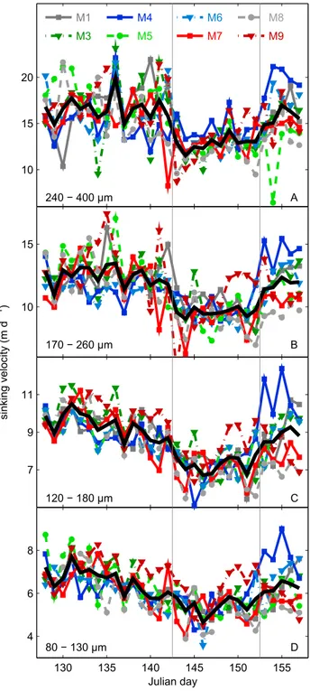
Aggregate sinking velocities averaged over the whole experiment were 6.1 (80–130μm), 8.6 (120–180μm), 11.4 (170–260μm), and 15.2 (240–400μm) m d¹, respectively, and increased with aggregate size (Figure S2B). Changes in sinking velocity over time are similar among the four size classes (Figure 6) reﬂected in the linear correlation between sinking velocities of different size classes (Figure S2C). Its temporal development mirrored changes in ρaggregate (see above and compare Figures 6 and 5E–5H). Thus, all relevant changes in aggregate sinking velocity measured in the settling columns were caused by changes in their density properties.

3.3. Ballasting of Sediment Trap Material

At the beginning of the experiment roughly 65% of the total sediment material weight were made up by organic matter, while silica and CaCO₃contributed 25 and 10%, respectively (Figures 5M–5P). The fraction of silica and CaCO₃decreased steadily until day 140 to ~12 and 7%, respectively. The continuous reduction of silica ballasting during this period was paralleled by the decline of diatoms and BSi in the water column (Figures 2B and 5N). The reduction of CaCO₃contribution in phase I was not reﬂected in a decrease ofE.

Figure 6.(A–D) Measured sinking velocities of the four size classes (with Figure 6D being the smallest). The black line is the mean sinking velocity calculated as the daily average of all mesocosms. The vertical grey lines separate the three phases. NO₃and PO₄³were added on day 142.

(12)

huxleyicell abundance (Figures 3E and 5O) but may instead either be attributable to (1) decreasing coccolith production rate at stableE. huxleyipopulation size, (2) the dwindling presence of calcifying mollusk larvae (Figure 4E), or (3) to a declining abundance of bacteria-derived CaCO₃precipitates [Heldal et al., 2012] (see also section 4.1.1).

Silica contribution to total density started to increase again on day 146, which was 4 days after the nutrient addition (Figure 5N). The increased share of silica material in the sediment trap of 15–25% shortly after the peak of the second bloom (Julian day 150) coincides with a decline of water column BSi as well as NANO I and NANO II abundances (Figures 2B, 3B, and 3D). Silica contribution decreased linearly after day 150 reﬂect- ing the decrease of BSi in the water column. Its contribution was 5–13% at the end of the experiment.

CaCO₃contribution to total density generally scaled positively withE. huxleyiabundance for the time after the nutrient addition until the end of the experiment. HighestE. huxleyi abundance in M4 translated to 28% CaCO₃ contribution to weight fraction of sediment trap material at the end of the experiment. In contrast, CaCO₃was not contributing at all to the material weight in M9 during this phase (Figure 5O), where E. huxleyiappeared in very low abundances (Figure 3E).

3.4. Relevance of Changes in Sinking Velocity for Particulate Matter Transfer Efﬁciency

Aggregate sinking velocities changed considerably in the course of the experiment in response to the plankton community succession (Figure 6). We formulated the one-dimensional carbonﬂux model (equation (9)) in order to assess whether changes within this scale could be relevant for particulate matter sequestration.

Results of this sensitivity analysis are shown in Figures S3A and S3B. The pattern of particle remineralization resembled a Martin curve, irrespective of the modeled sinking velocities. Flux attenuation was negatively correlated with sinking velocities (Figure S3A). Transfer efﬁciency between 100 and 1000 m depth increased by about 0.25% per 1% increase in modeled sinking velocity (Figure S3B).

4. Discussion

Linking plankton community structure with measurement of export-relevant parameters by means of in situ mesocosm studies has recently been identiﬁed as a research priority [Sanders et al., 2014]. We enclosed a natural plankton community in a Norwegian fjord and were able to follow its development for more than a month under close to natural conditions (see video byBoxhammer et al. [2015] to get an impression on the plankton community). This experiment is theﬁrst in a series of several (Swedish coast, 2013; Coast off the Canary islands, 2014; Norwegian coast, 2015), where sinking velocity measurements with high temporal resolution [Bach et al., 2012a] were linked with plankton community structure within the mesocosms. We will therefore not only address the major hypothesis and outcomes of the study (section 4.1) but also discuss limitations and illustrate potential improvements of the mesocosm approach (section 4.2).

4.1. Inﬂuence of the Plankton Community Structure on Aggregate Properties and Sinking Velocities 4.1.1. Was There a Transition from Ballast to Packaging-Dominated Control on Sinking Velocity?

Theﬁrst phytoplankton bloom was characterized by high BSi concentrations in the water column and a large copepod population developing from nauplii into adults. Aggregates sank relatively fast during this period, which appears connected to a large CaCO₃ and BSi ballast loading (Figure 5P) rather than low P_estimated(Figures 5I–5L).

Potential CaCO₃-forming organisms present in the mesocosms at this time comprisedE. huxleyi(Figure 3E), metazoan calciﬁers (Figures 4E and 4F), and bacteria which can contribute up to ~0.3μmol kg¹of inorganic CaCO₃as particles (1–100μm) in Raunefjord [Heldal et al., 2012] through the release of polyamines [Yasumoto et al., 2014]. We estimated CaCO₃supply byE. huxleyibased on the assumptions that each cell contributed a total of 2 pmol CaCO₃(1 pmol within the coccosphere plus 1 pmol as detached coccoliths [Balch et al., 1993]).

The presence of 52–185 cells mL¹ during the ﬁrst 7 days (Figure 3E) would result in a water column

coccolithCaCO₃standing stock of 0.1–0.37μmol L¹, whereas the corresponding CaCO₃accumulation rate in the sediment traps ranged from 0.012 to 0.052μmol L¹d¹during this period (CaCO₃sedimentation data not shown). We estimated that 8–37% loss of the_coccolithCaCO₃standing stock per day could fully account for the bulk CaCO₃recovered from the sediment traps during theﬁrst 7 days. Such a loss rate could have been easily compensated by new coccolith production by theE. huxleyipopulation [Bach et al., 2012b] inside the

(13)

mesocosms. Thus, CaCO₃ballast recovered from the sediment traps during theﬁrst 7 days could have potentially been supplied to a large extent byE. huxleyi. The relevance of other CaCO₃sources remains unclear, but since, for example, metazoan shells were sparse and have a lower carrying capacity for organic matter, they may not have been particularly efﬁcient ballast materials [Schmidt et al., 2014].

Opal ballast particles were generated by diatoms (mainlyArcocellulussp. andThallassiosirasp.), which were the only silicifiers present in noticeable quantity by this time. Both diatom frustules andE. huxleyicoccoliths are small (~3–15μm), which allows them to be more homogenously incorporated into an organic aggregate matrix and serve as efficient ballast particles [Schmidt et al., 2014]. Hence, we assume that relatively fast sinking during thefirst bloom was primarily due to opal ballasting by diatoms and presumably CaCO₃ballasting byE. huxleyi.

The contribution of BSi and CaCO₃to the total weight of sediment trap material was rapidly decreasing from

~27% (day 137) to 16% (day 140) after thefirst bloom. Sinking velocities, however, were not noticeably affected by the sudden decline in ballasting (Figure 6). The absence of a clear reduction of sinking velocities can be explained by decliningP_estimated(i.e., increasing aggregate compactness), which compensated for the reduction of BSi and PIC ballasting during this time (Figures 5I–5L). Interestingly, the estimated shift toward less porous aggregates happened when chlorophyllareached baseline levels and NO₃and PO₄³were close to (NO₃) or within (PO₄³) the detection limits (Figures 2A–2C). Therefore, we speculate that the decrease inP_estimatedcould have been caused by a transition in the food web from a diatom-dominated food web fueled by upwelled nutrients (new production) toward one, which was increasingly dependent on remineralized nutrients (regenerative production). Presumably, the shift toward regenerative production may have intensified recycling and led to a more thorough removal of fresh andfluffy components from the POC standing stock. This hypothesis is supported by observations of higher POC and PON contents in diatom-derived marine snow compared to aggregates containing more decomposed components [Alldredge, 1998]. The preferential removal offluffy components would lead to an accumulation of more den- sely packed material in the sinking material [Lam et al., 2011]. Additionally, this repackaging may have been further amplified by copepods feeding on sediment trap material since we counted increasing numbers of living copepods in the sediment trap samples at the point when chlorophyllaconcentrations consolidated at a temporal minimum after thefirst bloom (compare Figures 2A and 4D). Organic matter became sparse in the water column at this time so that more and more copepods may have detected the sediment trap as an additional food source [Lampitt et al., 1993].

4.1.2. Sinking Velocity Control Through Aggregate Porosity? The Potential Role of Plankton Community Structure

The addition of nitrate and phosphate to all mesocosms (Figures 2B and 2C) on day 142 initiated a second phytoplankton bloom. Diatoms were a prominent component in this second bloom (Figure 2B) as there was still dissolved silicate left in the system (~0.5μmol L¹on day 142). The loss rate of copepods through sedimentation declined during bloom buildup, suggesting that the animals were attracted by the fresh food growing in the water column and relied to a lesser extent on debris collected in the sediment trap.

Sinking velocities responded to these water column processes with a profound decline and reached experiment minima briefly after nutrient addition (Figure 6). To our surprise, these lowest velocities were sustained throughout the entire diatom bloom between days 142 and 152 even though increasing amounts of BSi ballast were collected in the sediment traps with a ballasting potential close to that observed during thefirst bloom (Figure 5N). The absence of a positive BSi ballast effect on sinking velocities during the diatom bloom could have three different reasons. First, BSi ballast was not integrated into the aggregate matrix. This is unlikely, however, considering that much of it originates from small diatoms (section 3.1), which should have a high potential to attach to organic matter due to their relatively high scavenging potential [Burd and Jackson, 2009;Schmidt et al., 2014]. Second, the dominant diatoms coagulated within aggregates actively downregulated their excess density in order to remain at higher light intensities during nutrient-fertilized growth as seen for large chain-forming species [Moore and Villareal, 1996]. This explanation is also rather unlikely, since large chains were hardly present in our study and decelerated sinking under nutrient-repleted conditions is a species-dependent, not a universal feature of diatoms [Bienfang et al., 1982]. Third, perhaps most likely seems to be that highP_estimated(Figures 5I–5L) decelerated sinking velocity and thus overcom- pensated the positive influence of mineral ballast during that time. This conclusion is also supported by

(14)

our daily inspections of the sediment trap samples, where we noted that the collected material looked like a ﬂuffy mush rather than a consortium of individual particles.

Comparing the succession ofP_estimatedduring bloom one (phase I) with that of bloom two (phase II + phase III) reveals a remarkably similar pattern.P_estimatedwas rather high in both blooms as long as the system was in a

“new production state,”where biomass buildup is fueled by upwelled or added inorganic nutrients.P_estimated decreased, however, when switching back to a“regenerative state”under low inorganic nutrient concentrations in the aftermath of a bloom (compare Figures 2B and 2C and Figures 5I–5L). These observations are in line with a growing body of literature that export of aggregates generated during the typical diatom spring bloom is relatively inefﬁcient due to their high porosity (i.e., low packaging) [Francois et al., 2002;Lam and Bishop, 2007;

Lam et al., 2011;Puigcorbé et al., 2015].

To further explore mechanisms controlling packaging we not only looked at the temporal development of P_estimatedbut also had a closer look on the differences among mesocosms. Differences were generally small and the overall trend was similar, but we noticed thatP_estimatedtended to be lower in those mesocosms, which harbored higher numbers of picophytoplankton (e.g., M5, M7, and M9; Figures 3A and 3C). In order to test this observation, wefirst calculated the biovolume of all phytoplankton groups (Figure 9), then calculated the ratio of groups smaller 2μm (PICO) to groups larger 2μm in diameter (NANO), and thereafter correlated the average PICO/NANO ratio with the averageP_estimated(Figure 7). We found a negative correlation between the PICO/NANO ratio andP_estimatedin all four aggregate size classes (Figure 7), which suggests that plankton communities with abundant picophytoplankton tend to generate more tightly packed aggregates than communities where a higher fraction of the biomass is accumulated in larger species. This observation is Figure 7.Influence of plankton community structure onP_estimated. Estimated cell diameters used for biovolume calculations (assuming spherical shape) wereSynechococcus= 1μm, picoeukaryotes = 1μm, NANO I group = 3μm, NANO II group = 10μm,E. huxleyi= 6μm, and cryptophytes = 7μm. Biovolume was subsequently calculated by multiplication of flow cytometry counts (Figure 3) with species-specific biovolumes. The sum of biovolume of species smaller than 2μm (Synechococcousand picoeukaryotes) divided by the sum of biovolume provided by species larger than 2μm (NANO I, NANO II,E. huxleyi, and cryptophytes) is the PICO:NANO ratio. Shown here is the PICO:NANO ratio andP_estimatedaveraged over the whole experiment with one line for each of the four aggregate size classes.

(15)

mechanistically reasonable because small aggregate components allow relatively little interstitial space between them [Burd and Jackson, 2009]. Furthermore, PICO-dominated communities usually prevail in regenerative systems, where particles potentially undergo a relatively large degree of biotic reprocessing and therefore a continuous compression [Lam et al., 2011]. With respect to particle matter export, low P_estimatedaggregates formed in a high PICO/NANO regime would promote transfer efficiencies as they prob- ably sink faster thanfluffy aggregates. Thus, the negative correlation between PICO/NANO andP_estimated (Figure 7) observed in our study may help to explain the numerous observations that low productivity regimes tend to generate particles with high transfer efficiencies [Francois et al., 2002;Lam and Bishop, 2007;Lomas et al., 2010;Lam et al., 2011;Henson et al., 2012a, 2012b;Maiti et al., 2013;Cavan et al., 2015;

Puigcorbé et al., 2015].

4.1.3. The Potential for Sinking Velocity Acceleration byE. Huxleyi-Derived CaCO₃Ballast

Phase III was characterized by decreasing chlorophyllaand BSi concentrations as well as treatment-specific developments within major phytoplankton and zooplankton types (Figures 3 and 4). The differential developments among mesocosms were reflected in particle sinking velocities, where those mesocosms which harbored significant E. huxleyi blooms generated aggregates with some of the highest sinking velocities measured during the entire study, while aggregate sinking velocities remained at a low level in mesocosms whereE. huxleyigrowth was muted (Figures 3 and 6).

The acceleration of sinking velocities in phase III was most likely due to CaCO₃ballast provided byE. huxleyi (Figure 8) and rather not caused by tight packaging becauseP_estimatedwas higher in those treatments with high CaCO₃availability (compare Figures 5I–5L with 5O). We used the positive correlations between particle sinking velocity andE. huxleyiabundance (Figure 8A) or sediment material PIC:POC ratio during phase III (Figure 8D) to estimate the influence ofE. huxleyi-dependent acceleration of particle sinking velocity on transfer efficiency with the one-dimensional particleflux model (equation (9)) derived in section 2.6. Therefore, slopes and theyintercepts of the four sinking velocities versus PIC:POC or cell abundance correlations (see Figures 8A and 8D) were plotted against average ESD of the respective size class. Slopes andyintercepts of the four correlations increased with average aggregate size (Figures 8B, 8C, 8E, and 8F), which is expected according to Stokes’law. With the slopes versus ESD (Figures 8B and 8E) and y intercepts versus ESD Figure 8.Influence of theE. huxleyiblooms on sinking velocities during phase III. (A) Sinking velocities of the four size classes (black triangles: 80–130μm; blue dots:

120–180μm; green squares: 170–260μm; red pyramids: 240–400μm) as a function of water columnE. huxleyiabundance. Each data point represents the phase III average of one mesocosm with error bars being standard deviations. Note that we calculated phase III averages (instead of using daily measurements during phase III) as we are unable to tell with what temporal delayE. huxleyicells arrive in the sediment traps. (B) Correlations between slopes and average ESD or (C)yintercepts and average ESD of the regressions calculated in Figure 8A. (D–F) The same results as in Figures 8A–8C, but in this case, sinking velocities are a function of PIC:POC ratio measured in sediment trap material. Note that data from individual days during phase III could be used in Figure 8D in contrast to Figure 8A because measurements of PIC:POC and sinking velocities were done with material collected on the same day.

(16)

(Figures 8C and 8F) correlations, we were able to parameterize the dependency of sinking velocities on either sediment material PIC:POC ratio or water columnE. huxleyiabundance (N_ehux) as

Sinkingvelocity_PIC:POC¼slope_PIC:POCPIC:POCþintercept_PIC:POC (11) and

Sinkingvelocity_ehux¼slope_ehuxN_ehuxþintercept_ehux (12) where slope_PIC:POCand slope_ehuxas well as intercept_PIC:POCand intercept_ehuxwere taken from regressions shown in Figures 8B, 8C, 8E, and 8F. TheE. huxleyi- or PIC:POC-dependent acceleration of sinking velocities can subsequently be included in the export model (equation (9)) by multiplying the sinking velocity_model term with the ehux_factoror the PIC:POC_factor, deﬁned as

ehux_factor¼slope_ehuxN_ehuxþintercept_ehux

intercept_ehux (13)

and

PIC:POC_factor¼slope_PIC:POCPIC:POCþintercept_PIC:POC

intercept_PIC:POC (14)

Hence,U_modelin equation (9) increases about a certain percentage throughout the entire water column, similar as has been simulated in the sensitivity analysis conducted in section 3.4. This time, however, sinking velocity is not increased by an arbitrary factor but scales withE. huxleyicell concentrations in the euphotic zone or the PIC:POC ratio of the sinking aggregates.

Sinking velocity acceleration was already profound under relatively lowE. huxleyiabundances or PIC:POC ratios (Figures 8A and 8D), which also considerably increased transfer efficiencies (Figure 9). For example, we estimated an acceleration of almost 40% for an increase in E. huxleyi abundance from 0 to 1500 cells mL¹or a PIC:POC increase of ~0.1 (Figures 8A and 8D). Such a ballast-mediated increase in sinking velocity could elevate transfer efficiencies from 14 to 24% (Figure 9). The key question now is: AreE. huxleyi cell densities of 1500 cells mL¹and the corresponding increase in PIC:POC exceptional or common in the Figure 9.Influence of theE. huxleyiblooms on transfer efficiencies during phase III calculated with the one-dimensional carbonflux model (section 4.1.3). (A) Flux attenuation as a function of differentE. huxleyi-dependent sinking velocity parameterizations (section 4.1.3; Figure 8a). The upper and lower horizontal grey lines indicate the bottom of the euphotic zone and sequestration depth, respectively. (B) Increase of transfer efficiency withE. huxleyiabundance in the euphotic zone. (C and D) The same results as in Figures 9A and 9B, but in this case, sinking velocities are a function of PIC:POC ratio measured in sediment trap material (section 4.1.3; Figure 8D).

(17)

oceans? Abundances of up to 1000 [Poulton et al., 2013], 1500 [Balch et al., 1991], and even 20,000 coccospheres mL¹ [Holligan et al., 1993] were counted during bloom seasons on the Patagonian Shelf, the Gulf of Maine, and south of Iceland (63°N, 20°W), respectively.Kopelevich et al. [2014] calculated thatE.

huxleyioften reaches abundances of 3000 cells mL¹or even more during the typical coccolithophore sum- mer bloom in the Black Sea. An estimated 3 mmol PIC m³ contributed by 1500 cells mL¹ (assuming 2 pmol PIC cell¹[Balch et al., 1993]) also compares reasonably well with data from the satellite studies by Moore et al. [2012] andHopkins et al. [2015], who found coccolithophore PIC of 1–10 mmol m³to be common on shelves and many regions of the open ocean during bloom season. Based on these assessments onE. huxleyi abundance we conclude thatE. huxleyi-associated particle sinking velocity accelerations of

~40% or even more are perhaps not unusual. Thus, the regional and/or seasonal occurrence ofE. huxleyi blooms may mark events of highly efﬁcient sequestration pulses.

4.2. Sinking Velocity Measurements of Mesocosm Sediment Trap Material: Uncertainties, Limitations, and Future Directions

4.2.1. Inﬂuence of Lithogenic Ballast Materials

Some of the highest sinking velocities of the entire experiment were measured during the first days (Figure 6). As lithogenic material has not been quantified in this study, it cannot be ruled out that the initially fast sinking rates are due to lithogenic ballast minerals enclosed while lowering the mesocosm bags at the beginning of the experiment. However, mesocosm bags were closed 4 days before thefirst sinking velocity measurement and the sediment traps were emptied on a daily basis until then. Artificial seeding of mesocosms with Saharan dust particles (99%<1μm in size) showed that fastest sinking dust particles are transferred to 9.5 m within hours [Bressac et al., 2012]. Smaller particles remained longer in the water column but also declined considerably within 2 days [Bressac et al., 2012]. Thus, if lithogenic ballast particles were present in relevant quantities at the beginning of our experiment, then most of it should have sunk out of the water column before thefirst sinking velocity measurement.

The Icelandic volcano Grímtsvötn erupted in the course of the experiment on 21 May. Part of the Grímtsvötn ash plume passed the Raunefjord area during the night from 24 to 25 May (days 144–145) with ash concentrations ranging from 200 to 4000μg m³air and ash particle sizes between ~1μm and 50μm [Tesche et al., 2012;Lieke et al., 2013]. Sinking velocities, however, remained low after the ash passage (Figure 5) for at least another 4 days, which is too long considering that particles within this size class should have arrived much earlier in the sediment trap. Furthermore, the acceleration of sinking velocity 4 days after the ash passage was inconsistent among mesocosms, which is in contrary to expectations in case of such a dust-seeding event. Thus, it is concluded that dust from the Grímtsvötn eruption was unlikely to have a signiﬁcant ballast effect on mesocosm aggregates, either because ash concentrations were too low or because they were insuf- ﬁciently collected by the mesocosms.

Based on these two lines of evidence we conclude that lithogenic ballast materials did not play a crucial role in the present study. Nevertheless, it is advisable to quantify their inﬂuence in mesocosm experiments on particle export because they may play an important role in other settings, where dust inﬂux is more likely.

4.2.2. Sampling-Associated Limitations and Potential Improvements

Prior to sinking velocity determination, aggregates had to be pumped from the sediment trap to the surface, carried to land in a bottle, and prepared for the measurements (see section 2.3). This procedure provoked aggregate fragmentation and reassembly, which potentially influenced aggregate porosity and density and likely influenced aggregate size. Potential effects on porosity and density should be relatively constant over time and thus of minor consequence on the trends observed in this study. The likely modification of the aggregate size structure prevented us from investigating if changes in the plankton community composition could influence aggregate sinking velocity through changes in aggregate size structure.

Our method to measure sinking velocities (as set up in this study) is restricted to particles from 80 to 400μm in ESD [Bach et al., 2012a]. Although particles of that size are responsible for a large fraction of organic matter export to depth, we missed the important inﬂuence of particles outside that range [Clegg and Whitﬁeld, 1990;

Ebersbach and Trull, 2008;Durkin et al., 2015]. In our study it is likely, however, that sinking velocities of aggregates>400μm would have shown a similar response to changing plankton community structure as the ones below this threshold as long as they are composed of smaller aggregate building blocks. The same principle should apply for aggregates <80μm but only until they become so small that they reach the size of