IHS Economics Series Working Paper 309
December 2014
Forecast combinations in a DSGE- VAR lab
Mauro Costantini Ulrich Gunter Robert M. Kunst
Impressum Author(s):
Mauro Costantini, Ulrich Gunter, Robert M. Kunst Title:
Forecast combinations in a DSGE-VAR lab ISSN: Unspecified
2014 Institut für Höhere Studien - Institute for Advanced Studies (IHS) Josefstädter Straße 39, A-1080 Wien
E-Mail: o ce@ihs.ac.atffi Web: ww w .ihs.ac. a t
All IHS Working Papers are available online: http://irihs. ihs. ac.at/view/ihs_series/
This paper is available for download without charge at:
https://irihs.ihs.ac.at/id/eprint/2911/
Forecast combinations in a DSGE-VAR lab
Mauro Costantini1, Ulrich Gunter2, and Robert M. Kunst3
1Brunel University
2MODUL University Vienna
3Institute for Advanced Studies, Vienna and University of Vienna
December 2014
All IHS Working Papers in Economics are available online:
https://www.ihs.ac.at/library/publications/ihs-series/
Economics Series
Working Paper No. 309
Forecast combinations in a DSGE-VAR lab
Mauro Costantini1, Ulrich Gunter2, and Robert M. Kunst3
1Department of Economics and Finance, Brunel University, Kingston Lane, Uxbridge, Middlesex, UB8 3PH, United Kingdom
2Department of Tourism and Service Management, MODUL University Vienna, Am Kahlenberg 1, 1190 Vienna, Austria
3Department of Economics and Finance, Institute for Advanced Studies, Stumpergasse 56, 1060 Vienna, Austria, and Department of Economics,
University of Vienna, Oskar Morgenstern Platz, 1090 Vienna, Austria
Abstract
We explore the benefits of forecast combinations based on forecast- encompassing tests compared to simple averages and to Bates-Granger combinations. We also consider a new combination method that fuses test-based and Bates-Granger weighting. For a realistic simulation design, we generate multivariate time-series samples from a macroe- conomic DSGE-VAR model. Results generally support Bates-Granger over uniform weighting, whereas benefits of test-based weights depend on the sample size and on the prediction horizon. In a corresponding application to real-world data, simple averaging performs best. Uni- form averages may be the weighting scheme that is most robust to empirically observed irregularities.
Keywords: Combining forecasts, encompassing tests, model selection, time series, DSGE-VAR model.
1 Introduction
Forecast combination is an attractive option for the improvement of forecast accuracy. A linear combination of two or more predictions often yields more accurate forecasts than a single prediction when useful and independent in- formation is taken into account (see Bates and Granger, 1969; Clemen, 1989;
Timmermann, 2006; Hsiao and Wan, 2014). Whereas the empirical evidence generally supports such combinations, there is less agreement on the opti- mal weighting rule in typical empirical situations. For example, Genre et al. (2013) support equal-weighted averages, while Hsiao and Wan (2014) see advantages for more sophisticated schemes, such as Bates-Granger weights.
We are interested in the potential gains in terms of predictive accuracy that can be achieved by combining forecasts on the basis of a multiple en- compassing test developed by Harvey and Newbold (2000) as compared to combinations based on simple uniform weights and on weights inversely pro- portional to squared forecast errors over a training sample, the procedure suggested by Bates and Granger (1969). Further, we consider a new hybrid procedure that eliminates rival models according to a forecast-encompassing test and then imposes Bates-Granger weights on the remaining candidates.
Convincing demonstrations in support of a forecasting procedure are a
challenging task. Horse races for empirical data are subject to sampling vari- ation and thus to arguments of statistical significance. Simulations, on the other hand, yield exact results but their relevance critically hinges on the plausibility of their design. Here, we compare the techniques on data gener- ated by a macroeconomic DSGE-VAR model, whose relevance as a potential generator of actual macroeconomic data is widely supported by economic the- orists. A drawback of this complex generator is that simulations are costly in terms of computer time, such that assessing the effects of varying the design becomes unattractive. For this reason, we also apply the methods to cor- responding empirical data in a control experiment. All forecast evaluations focus on predicting real gross domestic product (GDP), the output variable of central interest in macroeconomic analysis.
In a related study, Costantini and Kunst (2011) use French and U.K.
data in order to investigate whether and to what extent combined forecasts with weights determined by multiple encompassing tests help in improving prediction accuracy, against the backdrop of uniform weighting. They report some benefits for test-based weighting in one of their two data sets. We are interested in finding out whether such benefits for test-based weighting can be regarded as systematic.
The DSGE-VAR model that is used as the generating mechanism for our data constitutes a hybrid model that builds on the DSGE (dynamic stochas- tic general equilibrium) model suggested by Smets and Wouters (2003) and fuses it to a VAR (vector autoregressive) model following Del Negro and Schorfheide (2004). Our interest in using DSGE models for generating data arises from the ubiquitous usage of this modeling approach in current macroe- conomic practice, which makes it plausible to view designs of this type as approximating a realistic macroeconomic world. Over the past two decades, these so-called New Keynesian models have been spreading out in the macroe- conomic literature, varying in their levels of complexity as well as in the specific focus of application, such as policy analysis (see, e.g., Smets and Wouters 2003) or forecasting (see, e.g., Smets and Wouters 2004). In the empirical implementation of DSGE models, Bayesian estimation techniques play a major role (see An and Schorfheide, 2007, for a survey). For other authors who take up a comparable idea of using DSGE models as a labo- ratory for studying effects in a realistic environment, see Justiniano et al.
(2010) or Giannone et al. (2012). In contrast to most comparable studies, however, we rely on a hybrid DSGE-VAR specification due to Del Negro and Schorfheide (2004), as it has evolved that these DSGE-VAR models attain a
more realistic representation of actual data than the pure DSGE variant.
Our forecasting evaluation assumes that the forecaster has no knowledge of the underlying DSGE-VAR model and considers four time-series specifica- tions as potential approximations to the generating mechanism: a univariate autoregression; two bivariate autoregressions that contain the target vari- able and one of two main indicator variables, the (nominal) interest rate and the rate of inflation; and a factor-augmented VAR (FAVAR) model that adds three estimated common factors to output to form a four-dimensional VAR. This design implies that the true model is not contained in the toolbox considered by the forecaster.
The contrast between the sophisticated generating mechanism and the comparatively simple prediction models is deliberate, as it is representative for the widespread empirical situation. A crucial feature in this regard is the quality of approximation of the dynamic behavior of DSGE models by VAR or FAVAR models, which has been studied by several authors. For example, Boivin and Giannoni (2006) interpret the FAVAR as the reduced form of a DSGE model in the context of short-run forecasting. Gupta and Kabundi (2011) forecast South African data using a DSGE model and FAVAR variants as rival models and find that the FAVAR models outperform DSGE. We
emphasize, however, that we do not address the issue of DSGE as a prediction device—which is a topic of current interest in the forecasting literature—but we rather use the DSGE-type structures as realistic simulation designs.
From the four models, the forecaster is assumed to form weighted aver- ages for the target variable of output. To this aim, forecast-encompassing regressions (see Section 2) are run in all directions, encompassed models are eliminated as determined by F-statistics and a specific significance level, and the surviving models are averaged uniformly. The multiple encompassing test of Harvey and Newbold (2000) is also considered by Costantini and Pappalardo (2010), who use it to corroborate their hierarchical procedure for forecast combinations that is based on a simple encompassing test of Harvey et al. (1998). By contrast, the procedure considered here attains complete symmetry with respect to all rival forecasting models, as the multiple encom- passing test is run in all directions.
The test-based elimination procedure is compared to three alternative techniques: (a) the unweighted average; (b) a weighted average with weights determined by the MSE (mean squared error) over a training sample as sug- gested by Bates and Granger (1969); (c) a two-step procedure with test-based elimination followed by Bates-Granger weighting of the remaining candidates.
This latter construction is a new technique, and an assessment of its merits is of particular interest.
We evaluate the forecasts for various sample sizes ranging from 40 to 200 observations, i.e. for a range that may be typical for macroeconomic forecasting, on the basis of the traditional moment-based criteria MSE and MAE (mean absolute error) and also by the incidence of better predictions.
For the test procedure, we consider significance levels ranging in 1% steps from 0—which corresponds to uniform weighting—to 10%. Simple averages are often reported to be difficult to beat (see de Menezes and Bunn, 1993;
Clements and Hendry, 1998; Timmermann, 2006; Genre et al., 2013).
In summary, our experiment is of interest with regard to two aspects: first, it assesses the value of forecast combinations based on multiple encompassing in a realistic DSGE-VAR design; second, it assesses the effects of dimension reduction in the spirit of FAVAR models on forecast accuracy.
The plan of this paper is as follows. Section 2 outlines all methods: the forecast-encompassing test, the weighting scheme based on that test, and the rival prediction models that are to be combined. Section 3 expounds the simulation design, with details on the DSGE-VAR specification provided in an appendix. Section 4 presents the results of the prediction evaluation.
Section 5 reports an empirical application. Section 6 concludes.
2 Methodology
2.1 Encompassing test procedure for forecasting com- bination
This section presents the encompassing test procedure used to determine the weights in the combination forecast. The procedure is based on the multiple forecast encompassing F–test developed by Harvey and Newbold (2000).
Consider M forecasting models that deliver out-of-sample prediction er- rors e(k)t , k = 1, . . . , M, for a given target variable Y, with t running over an evaluation sample that is usually a portion of the sample of available obser- vations. Then, the encompassing test procedure uses M linear regressions:
e(1)t =a1(e(1)t −e(2)t ) +a2(e(1)t −e(3)t ) +. . .+aM−1(e(1)t −e(M)t ) +u(1)t , e(2)t =a1(e(2)t −e(1)t ) +a2(e(2)t −e(3)t ) +. . .+aM−1(e(2)t −e(M)t ) +u(2)t ,
. . .
e(M)t =a1(e(M)t −e(1)t ) +a2(e(Mt )−e(2)t ) +. . .+aM−1(e(M)t −e(Mt −1)) +u(M)t . (1)
These homogeneous regressions yield M regression F statistics. A model k is said to forecast-encompass its rivals if the F statistic in the regression with dependent variablee(k)t is insignificant at a specific level of significance.1 Following the evidence of the forecast-encompassing tests, weighted average forecasts are obtained according to the following rule. If F–tests reject their null hypotheses in all M regressions or in none of them, a new forecast will be formed as a uniformly weighted average of all model-based predictions.
If some, say m < M, F–tests reject their null, only those M −m models that encompass their rivals are combined. In this case, each of the surviving models receives a weight of (M −m)−1.
2.2 Bates-Granger weighting
Bates and Granger (1969) introduced a combination method that is typical for the so-called ‘performance-based combinations’ and assigns higher weights to forecasts with better forecasting track records:
wm,T = MSEm,T−1 PM
m=1MSEm,T−1 , (2)
1Harvey and Newbold (2000) use the wording ‘forecast-encompassing’ for the null hy- pothesis of the F test. We prefer to focus on empirical forecast-encompassing defined by non-rejection of the null and to use ‘encompassing’ in short.
whereMSEm,T denotes the mean squared error that evolves from forecasting based on model m from a sample ending in T. Recently, Hsiao and Wan (2014) presented some evidence in favor of this simple and appealing method.
Both Bates-Granger weighting and the encompassing-test approach ac- count for the performance over a training sample. The main difference is that the encompassing test eliminates uninformative rival models completely, while Bates-Granger assigns them a smaller weight. On the other hand, each of the models that was not eliminated obtains the same weight in the test- based scheme, while Bates-Granger weighting tries to distinguish between good and excellent models. Thus, it appears worth while to process the two ideas simultaneously.
This new hybrid procedure eliminates non-informative rivals in a first step, but then uses Bates-Granger weighting on the remaining models. Note that the weights should still sum to unity, so formula (2) holds in the second step with M representing the models that have not been eliminated.
In summary, we consider four forecast combination methods: (i) uniform averages of all models; (ii) elimination via forecast-encompassing; (iii) Bates- Granger weighting; (iv) a two-step procedure that combines (ii) and (iii).
2.3 The forecasting models
Forecasts are based on four classes of time-series models and on combinations of representatives from these four classes that have been estimated from the data by least squares after determining lag orders by information criteria.
As information criteria, we employ the AIC criterion by Akaike and the BIC criterion by Schwarz (see L¨utkepohl, 2005, section 4.3).
The first model class (model #1) is a univariate autoregressive model for the targeted output series. The second and third model are two bivariate vector autoregressive models (VAR). Model #2 contains output and inflation, and model #3 contains output and the nominal interest rate. This choice of added variables has been motivated by the fact that inflation and the interest rate are often viewed as main economic business-cycle indicators and they are also more often reported in the media than the remaining variables of the DSGE system.2
The fourth and last model class (model #4) is a factor-augmented VAR (FAVAR) model. Suppose that Yt is the target variable to be predicted (GDP), whileFtis a vector of unobserved factors that are assumed as related to a matrix of observed variables X by the linear identity F = XΛ with
2These variables are mentioned in Section 3.1 and listed in appendix A.
unknown Λ, such that the column dimension of F is considerably smaller than that of X. A FAVAR model can be described as follows:
Φ(L)
Yt
Ft
=εt, (3)
where Φ(L) = I −Φ1L −. . .− ΦpLp is a conformable lag polynomial of finite order p. Ldenotes the lag operator, andI denotes the identity matrix.
Equation (3) defines a VAR in (Yt, Ft′)′. This system reduces to a standard univariate autoregression forYtif the terms in Φ(L) that relateYttoFt−j, j = 1, . . . , pare all zero. Equation (3) cannot be estimated directly, as the factors Ft are unobserved.
The proper estimation of the models requires the use of factor analysis (see Stock and Watson, 1998, 2002). The estimation procedure consists of two steps. In the first step, the factors F are estimated using principal component analysis. The minimum of the BIC(3) criterion developed by Bai and Ng (2002) determines the number of factors, i.e. the dimension of F. In the second step, the FAVAR model is estimated by a standard VAR method with Ft replaced by the estimate ˆFt that is available from the first step.
Thus, in our forecast experiments, the FAVAR forecasts rely on VAR models for the target output series and three additional factors that have
been formed from combinations of the nine remaining observable variables of the DSGE system that is detailed in appendix A. The choice of the number three has been motivated by the fact that it is customary not to use more than a maximum of three factors if nine series are available. In fact, we use three as an upper bound on the factor dimension but the information criterion BIC(3) always selects the maximum dimension. This indicates that the variables in the DSGE system are quite heterogeneous and that the information in the system cannot be easily condensed to a low dimension.
The FAVAR formed using this procedure has a dimension of four. Indeed, we considered an alternative variant with two factors only for all of our simulation designs. Excepting some designs at the smallest samples, however, the three-factor version yields the better forecasting performance. For this reason, we report the three-factor version exclusively.
The four rival model classes are incompletely nested, with models #2 to
#4 representing generalizations of model #1 and models #2 and #3 repre- senting special cases of #4. Due to the lag selection that tends to choose larger lag orders for the lower-dimensional model, however, the general situ- ation is to be seen as non-nested.
For a given considered sample size of N, all models are estimated for
samples of size 3N/4 toN−h−1 using expanding windows, withh = 1, . . . ,4 denoting the prediction horizon. Then, the next observation at position t = 3N/4 + h, . . . , N −1 is forecasted. Thus, an original sample of size N = 200 yields a one-step forecasts for observation t = 151 based on 150 observations, then for t = 152 based on 151 observations etc., finally for t = 199 based on 198 observations. It follows that the reported accuracy measures average estimates of different quality. Our design represents the action taken by a forecaster who observes 199 data points and targets the forecast for the observation atN = 200 by optimizing her combinations of the basic rival forecasts to this aim. In other words, the report of the forecasts from the basic rival models is to be seen as an intermediate step.
For each replication, we consider combinations of forecasts based on weighted averages of the four basic rival models for the observations at time points t = N. These combinations are determined by the forecast- encompassing tests outlined above. For the F tests, we consider significance levels of k∗0.01 with k = 0, . . . ,10. The value k = 0 corresponds to a uni- form average, as no F statistic can be significant at the 0% level and hence models always encompass all other models. By contrast, k = 10 corresponds to a significance level of 10%. At sharp levels, the null remains often unre-
jected, and many combinations will be uniform. At looser levels, rejections become more common, and some models will be excluded from the average.
At extreme levels, no model will encompass and weights will again tend to be uniform. We do not consider levels beyond 10%, however, as these are unlikely to be of practical use, and some unreported experiments insinuate that they do not improve predictive accuracy.
3 The data-generating process
Details on the DSGE-VAR model specification that underlies our simulations are provided in the appendix A.
3.1 The DSGE-VAR simulation design
The original medium-scale closed-economy DSGE model of the Euro area by Smets and Wouters (2003) was estimated from quarterly data by Bayesian techniques. At first sight, it appears to have two desirable properties for cre- ating artificial data, namely relevance in macroeconomics due to widespread usage and an attractive level of complexity.
Nonetheless, whereas Smets and Wouters (2003) find that their DSGE
models attain higher marginal likelihoods than VARs, Del Negro et al. (2007) warned that such findings crucially hinge on the observation sample. Even relatively sophisticated DSGE models are not robust against small changes in the sample period, hence a non-negligible degree of misspecification in DSGE models is apparent. In consequence, policy recommendations and forecasts based on this model class could be biased, and the empirical plausibility of artificial data generated by such a model may be impaired. Moreover, Smets and Wouters (2007) find that the estimates for some of the model parameters differ considerably between the ‘Great Inflation’ (1966:1–1979:2) and ‘Great Moderation’ (1984:1–2004:4) subsamples in US data, which casts doubt on the validity of approximating the actual economy by a DSGE model with time-constant parameters.
One way of addressing this misspecification issue is to replace the pure DSGE data-generating process by a hybrid DSGE-VAR that is known to be much less sensitive to changes in the observation period and also typically attains a higher marginal likelihood than both VAR and DSGE specifications (see Del Negro et al., 2007). The DSGE-VAR developed by Del Negro and Schorfheide (2004) and Del Negro et al. (2007) is a Bayesian VAR (BVAR) that uses the information provided by a DSGE model as an informative prior
for BVAR estimation. The impact of the DSGE information relative to the actual sample information is measured by a hyper-parameter ℵ ∈ (0,∞], which can either be kept fixed during estimation or estimated together with the DSGE model parameters (see Adjemian et al., 2008). A value of ℵ close to 0 corresponds to an unrestricted VAR at the one extreme, whereas a value of ℵequal to∞ corresponds to the VAR approximation of the DSGE model at the other extreme (see Del Negro et al., 2007).
The misspecification of the DSGE model class also shows in the optimal weight of the DSGE information for constructing the DSGE-VAR prior of ℵ∗ = 1.25 for the sample from 1974:2–2004:1 in Del Negro et al. (2007), which reflects an optimal impact of the information provided by the DSGE model of around 55% for DSGE-VAR estimation. For the derivation of the DSGE-VAR prior and posterior distributions as well as for a more technical description of the DSGE-VAR methodology, see Del Negro and Schorfheide (2004) and Del Negro et al. (2007).
Our aim is to generate artificial data that are empirically plausible across countries and sample periods. We therefore apply the subsequent three-step DSGE-VAR procedure while employing the Dynare preprocessor for Matlab, which is downloadable in its current version from http://www.dynare.org:
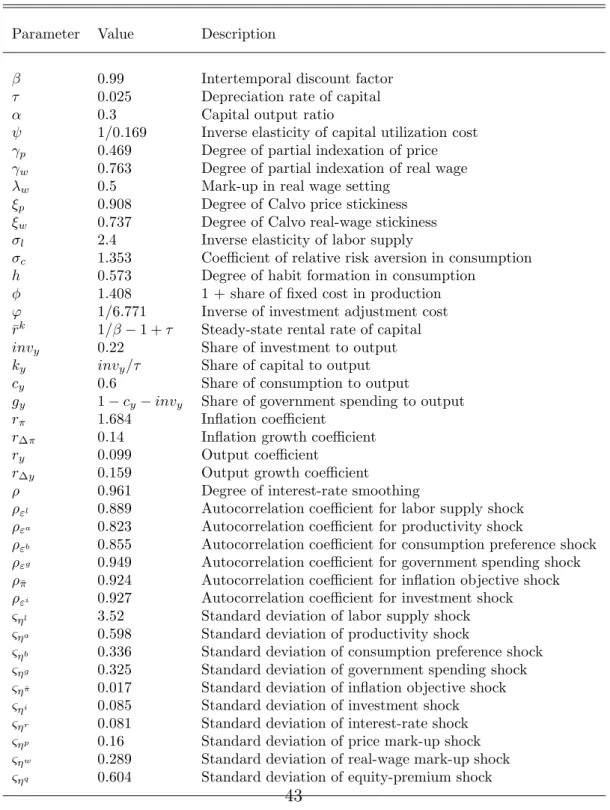
Step 1. We generate 2,000 time series, each of length 1,100, for ten key macroeconomic variables (consumption ˆC, real wage ˆw, capital ˆK, in- vestment ˆI, real value of installed capital ˆQ, output ˆY, labor ˆL, inflation ˆπ, rental rate of capital ˆrk, and gross nominal interest rate ˆR) from the original Smets and Wouters (2003) model as laid out in appendix A. In line with the source literature, hats on variables denote percentage deviations from the non-stochastic steady state.
Step 2. Discarding the first 100 observations of each of the 2,000 time series as burn-in draws, the remaining T = 1,000 observations serve as the data sample for estimating a DSGE-VAR of lag order p = 2 via Bayesian techniques. The posterior distribution of a DSGE-VAR model cannot be de- termined analytically, hence a Monte-Carlo Markov chain sampling algorithm has to be invoked to simulate the distribution of the vector of DSGE-VAR model parameters (for a survey on Bayesian inference in DSGE models see An and Schorfheide, 2007). In particular, we adopt a Metropolis-Hastings algorithm with two parallel Monte-Carlo Markov chains, each consisting of 55,000 draws. The first half of the draws are discarded before computing the posterior simulations. Roberts et al. (1997) find the optimal acceptance rate of draws at 0.234, which is met approximately across simulations.
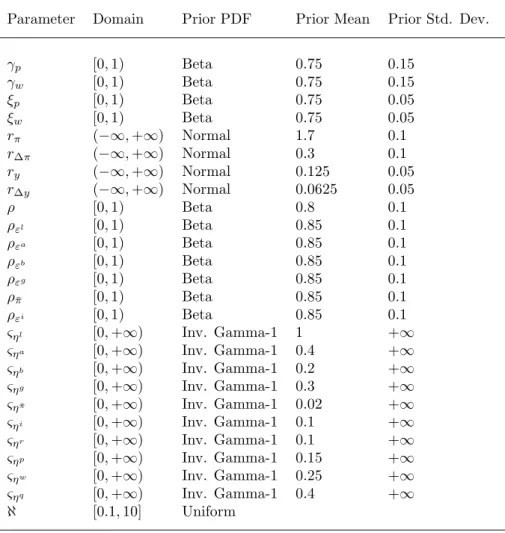
The DSGE model used for constructing the DSGE-VAR prior again is the model by Smets and Wouters (2003) as given by equations (A.1)–(A.10) in appendix A, with all parameters explicitly listed in Table 1. Due to the computational burden associated with 2,000 full-fledged Metropolis-Hastings simulations, we declare our target variable of interest ( ˆY), the two additional variables used in the bivariate VAR forecast models ( ˆR,π), and two auxiliaryˆ variables ( ˆw,rˆk) as the only observed variables, i.e. there arem= 5 observed variables altogether. We further restrict the number of free parameters to those listed in Table 2. Concerning the prior probability densities as well as the prior means and standard deviations of the DSGE model parameters, we again follow Smets and Wouters (2003).
In line with Adjemian et al. (2008), we choose to estimate the hyper- parameter ℵalong with the so-called ‘deep’ parameters of the DSGE model.
We assume a uniform distribution for the hyper-parameter between ℵ= 0.1, corresponding to an impact of the DSGE model information of about 10%, and ℵ= 10, corresponding to an impact of the DSGE model information of about 90% (note that, as in Adjemian et al., 2008, the minimum value to obtain a proper prior ℵmin ≥ (mp+m)/T = 0.015 is satisfied). All other parameters listed in Table 1 are kept fixed at the indicated values during
estimation.
Step 3. After retrieving the posterior distributions of the model pa- rameters for each of the 2,000 replications, we generate time series of length 1,100 for the ten macro variables using the pure perturbation algorithm of Schmitt-Groh´e and Uribe (2004). In this step, parameter values are set at the means of the posterior distributions.
This step is repeated 2,000 times to obtain 2,000 new time series of ar- tificial data. Whereas the first 100 observations of each time series are dis- carded as starting values, the remaining 1,000 observations are separated into shorter non-overlapping time series. Thus, the number of replications depends on the sample size. For the largest sample size of N = 200, 10,000 replications are available for our forecasting experiments. At the other ex- treme, for the smallest considered sample size of N = 40, the number of available replications increases to 50,000. The sample size N is varied over 20∗j for j = 2,3, . . . ,10. Samples smaller than N = 40 would not admit any useful forecasting evaluation, due to the relatively high dimension of the system.
If the procedure is interrupted after step 1, it delivers pure DSGE data.
By construction, the DSGE weight in the final DSGE-VAR model is com-
paratively large, typically around 87%. Nevertheless, the VAR contribution turns out to be important for forecasting performance.
4 Results
This section consists of three parts. First, we focus on the relative forecasting performance of the four basic rival models. The second subsection looks at the weights that these rival models obtain in the test-based forecast combi- nations. The third part considers the performance of the combined forecasts in detail.
4.1 Performance of the rival models
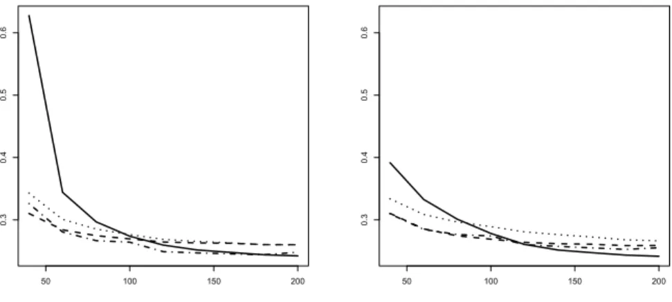
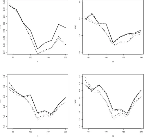
Based on the evaluation of mean squared errors, Figure 1 shows that the factor VAR model dominates at larger sample sizes in all designs, that is for AIC as well as BIC, and the same holds for the unreported two-factor version.
Figure 1 refers to the full DSGE-VAR version of the model. Comparable graphs for the pure DSGE model are similar and therefore omitted.
The three factors identified by the FAVAR algorithm vary considerably across replications. A rough inspection of the average weights of observed
variables shows that the first factor tends to incorporate investment I and the capital stock K. Even the second factor tends to assign large weights to I and to K, with some contributions from wages W and the rental rate rk. The third factor focuses on consumption C and on wages W, with some further contributions from the labor force L and the real value of capital Q.
In small samples, the univariate autoregression dominates but it loses ground as the sample size increases. Among the two bivariate VAR models, a clear ranking is recognizable. Model #3 with output and nominal interest rate achieves a more precise prediction for output than model #2 with output and inflation. This ranking is due to the structure of the DSGE model that assumes stronger links between output and the interest rate than between output and inflation. In fact, model #3 is pretty good for intermediate samples and can compete with the FAVAR specification at all but the largest samples, particularly in the AIC variants.
By contrast, the FAVAR performance is extremely poor in small samples, slightly worse with AIC than with BIC. AIC selects the more profligate spec- ification, with the largest number of free parameters to be estimated. For BIC order selection, FAVAR overtakes its rivals for good around N = 100, whereas slightly larger samples are needed for AIC.
Both graphs in Figure 1 use a common scale, which admits a rough com- parative visual assessment of the four variants. An obvious feature is the inferior performance of AIC in small samples, due to parameter profligacy.
In large samples, AIC and BIC perform similarly for the FAVAR model.
BIC selection, however, becomes less attractive for its less informative rival models that would need longer lags for optimizing their predictions.
Figure 1 restricts attention to single-step prediction. Results for longer horizons are qualitatively similar and are not reported. They are available upon request.
4.2 Weights in the combination forecasts
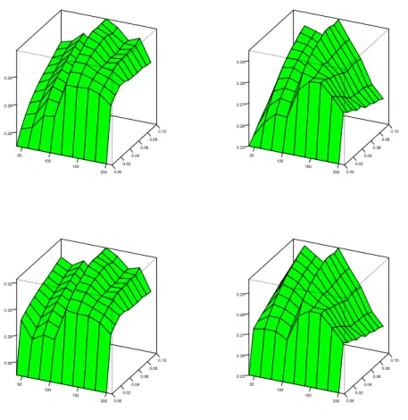
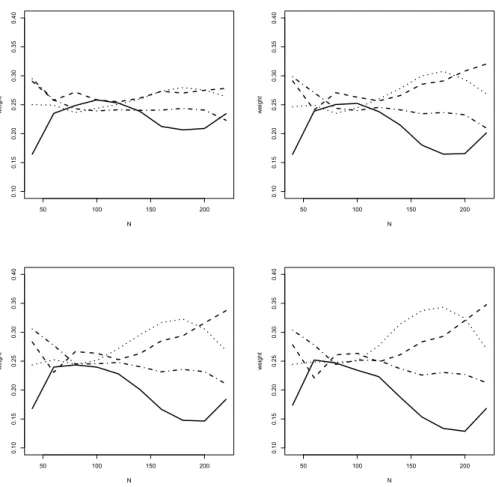
The univariate model is best for small samples, the FAVAR is best for large samples. Thus, one may expect that the FAVAR model receives a stronger weight in the encompassing-test weighting procedure, as the samples get larger.3 The upper graphs in Figure 2 show that this is indeed the case.
There are slight differences between the AIC and the BIC search. AIC implies a share of FAVAR of less than 25% for N = 40, meaning that the FAVAR
3Ericsson (1992) showed that the null hypothesis of the forecast encompassing test is a sufficient condition for forecast MSE dominance.
is often encompassed. BIC, on the other hand, chooses the proportional share even for N = 60 and N = 80. While for BIC order selection the less informative rivals outperform the FAVAR model in small samples with respect to the MSE criterion (see Figure 1), this behavior does not entail forecast encompassing, due to the heavily penalized and thus typically low lag orders. Otherwise, reaction is fairly monotonic in the sense that the FAVAR share increases with rising N and also with looser significance level.
As the significance level increases, weights diverge from the uniform pat- tern. We note, however, that even at 10% andN = 200 the weight allotted to the FAVAR model hardly exceeds 40%. This value is an average over many replications with uniform weighting and comparatively few where weights of 1/3, of 1/2, or even of one are allotted to FAVAR.
If the elimination via forecast encompassing is combined with Bates- Granger weights, one may expect a boost in the weight differences. The lower graphs in Figure 2 show that this is not really the case. Average weight preferences for specific models remain moderate, and the final weights after the second step are hardly affected on average, maybe excepting a stronger downweighting of the FAVAR model at the smallest sample sizes. This re- silience of average weights across procedures does not imply that the same
weights have been allotted for the same trajectories, and the next subsection will demonstrate that the overall MSE is indeed affected. The combined pro- cedure tends to assign the weights more accurately, even though the average weights remain identical.
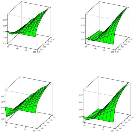
Whereas the weights for the univariate model and the bivariate VAR with inflation monotonically decrease with increasing N, weights for the bivariate model #3 with the interest rate peak for intermediate samples and are over- taken by FAVAR as N exceeds 120. Contrary to the FAVAR weights, they rise fast at small significance levels and then level out. Model #3 captures the essence of the DSGE-VAR dynamics at reasonable sample sizes well, and if it wins the encompassing tournament it does so typically at sharp significance levels. Figure 3 provides a summary picture of the weight allotted to model
#3 and demonstrates that this model remains competitive in larger sam- ples, with weights decreasing only slowly as N approaches 200, particularly in the AIC variant, thus confirming the impression from Figure 1. Again, we note the robustness of average weights when the two-step procedure with Bates-Granger weighting of non-eliminated models is used rather than the single-step elimination method.
Figures 2 and 3 refer to the full DSGE-VAR version of the model. With
regard to the FAVAR model, comparable graphs for the pure DSGE model are similar. Model #3, however, receives substantially more support in the pure DSGE design. It is conceivable that the comparatively large weights for this model even for N = 200 are responsible for the poorer performance of the test-based procedure that is reported in the following subsection.
When the prediction horizon grows, the main features of Figure 2 and 3 continue to hold, with one noteworthy exception. For larger samples, Figure 2 shows a smooth increase of the weight allotted to the FAVAR model with rising significance level. At larger horizons, this slope steepens, such that even at the 1% level a considerable weight is assigned to FAVAR. The larger weight allotted to FAVAR coincides with a lesser weight assigned to the bivariate model #3. This stronger discrimination among rival models affects the accuracy comparison to be reported in the next subsection.
4.3 Performance of test-based weighting
In order to evaluate the implications of the test-based method for forecasting, we use three criteria: the mean squared error (MSE), the mean absolute error (MAE), and the winning incidence. Generally, the MAE yields similar qualitative results as the MSE and we do not show the MAE results in detail.
The qualitative coincidence of MAE and MSE naturally reflects the normal distribution used in the simulation design.
Our graphical report is restricted to the DSGE-VAR design. For the DSGE design without the VAR step, the main qualitative features are similar, with support for test-based elimination however growing more impressively as the forecast horizon increases. All detailed results are available upon request.
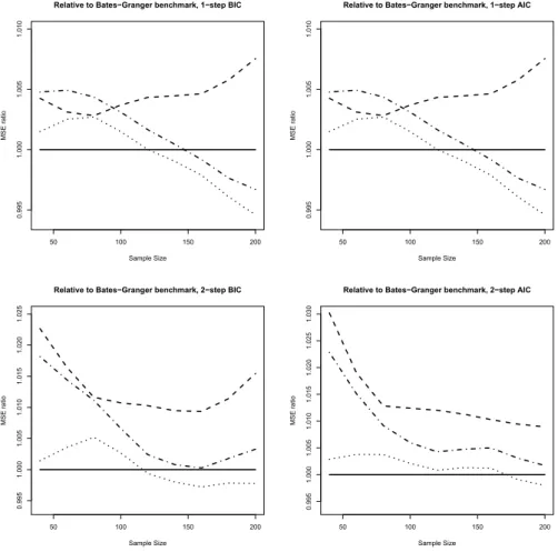
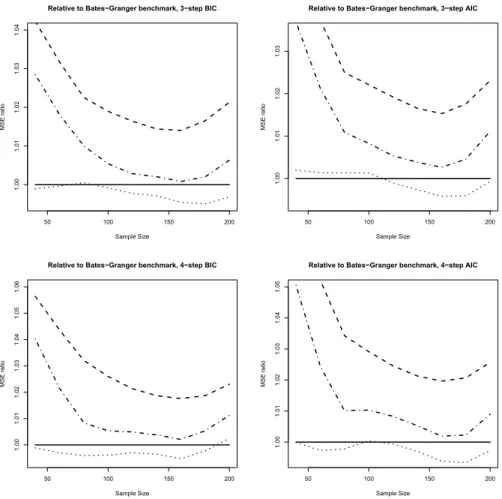
Figures 4 and 5 show ratios of the MSE achieved by all considered proce- dures relative to the benchmark of Bates-Granger weights: uniform averages, test-based elimination followed by uniform weights, test-based elimination followed by Bates-Granger weights. The graphs address AIC and BIC order selection in parallel, as we view the two criteria as two inherently differ- ent approaches, and thus do not report comparisons between AIC and BIC performance. Typically, BIC dominates AIC for the smallest sample sizes, while AIC performs better for N >80, which is well in line with the known forecast-optimizing property of AIC. All these figures focus exclusively on testing at the 1% significance level, as this is the value at which prediction accuracy measures are optimal almost for all specifications.
For single-step prediction (see the upper panels of Figure 4), the test- based procedures clearly benefit from larger sample sizes. At N ≥ 100, the
combined scheme is best, while for smaller samples the simple Bates-Granger cannot be beaten. For N ≥ 120, even the test-based weighting procedure with uniform weights of survivors beats the benchmark. At all sample sizes, naive uniform weights perform less convincingly, coming in last for larger samples, although the differences are not too large at less than 1%. We again note the advantage of simulation, as such differences may often be too small to be significant in an empirical investigation, while they are clearly larger than the sampling variation in our simulation design.
For two-step prediction (see the lower panels of Figure 4), relative differ- ences increase to around 2%, but the dominance of the combined procedure at larger samples becomes less convincing. The test-based weighting scheme is unable to beat the Bates-Granger benchmark at any sample size, and pure uniform averages rank last in all specifications. We note that we decided to use the Bates-Granger weights as well as the elimination procedure on two-step predictions proper, as we think this is more logical than basing all procedures on single-step predictions. This implies that the selected pre- diction models as well as their relative weights differ at different horizons.
The results suggest that the downweighting of poorly performing prediction models tends to be more important than eliminating the worst models.
If the step size increases, the occurrence of ties among the procedures becomes less prominent. This, in turn, leads to a clearer separation with regard to the accuracy ensuing from prediction models. The weight allotted to the best model, in large samples the FAVAR model, increases.
The impression that larger prediction horizons benefit the test-based pro- cedure is confirmed for the three-step prediction that yields the graphs in the upper part of Figure 5. Test-based weighting dominates uniform weights at all sample sizes and specifications. Bates-Granger weighting is clearly bet- ter than test-based weighting, and the hybrid two-step method even beats Bates-Granger at most sample sizes. These features are slightly enhanced for the four-step predictions summarized in the lower part of Figure 5. Even for four steps, relative differences at N = 100 remain around 3%.
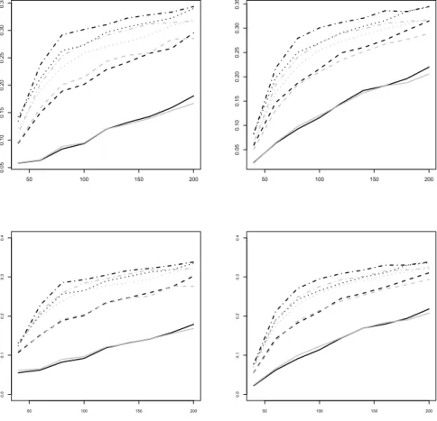
The criteria MAE and MSE are summary statistics, and they are based on moments of the error distributions. A lower MSE may be attained by a forecast that is actually worse in many replications but wins few of them at a sizeable margin. Therefore, we also consider the direct ranking of absolute errors. The incidence of a minimum among all levels could indicate which level is more likely to generate the best forecast. There are many ties, how- ever, so we only report the direct comparison for the 1% test-based weighting
in more detail. The upper graphs in Figure 6 show the frequencies of the two models of generating the smaller prediction error for the variants without Bates-Granger weights, whereas the lower graphs refer to the variants with Bates-Granger weights. Among others, Chatfield (2001) advocated the usage of the winning incidence as a measure of predictive accuracy.
For one-step forecasts, Figure 6 demonstrates that the differences in MSE reported above are due to comparatively few replications. Ties are many even for large samples (around 70%) and are the rule for small samples (around 90%). At small samples, no advantage for the test-based scheme is recognizable. At large samples, test-based weighting gains some margin over its rival but fails to impress.
In line with the MSE graphs, also the ‘winning frequency’ for the test- based scheme improves at larger forecast horizons. At two steps, the two schemes are still comparable. There is a slight advantage for the encompass- ing test in the BIC versions, while uniform weighting is remarkably strong in the AIC versions. At three and four steps, however, the test-based procedure gains a sizeable margin even for small samples. Ties become less frequent and their frequency falls to around 30% at horizon four and larger samples.
In summary, at larger prediction horizons test-based weighting becomes
increasingly attractive. At short horizons, the merits of test-based weighting are most pronounced for very small samples, where the accuracy of prediction is low, and at larger samples, where weighting becomes reliable.
5 Application to empirical data
This section reports on an application of the forecast combination techniques to empirical data that are the counterpart to the simulated data that underlie the DSGE-VAR model. This experiment can be interpreted in either of two ways. Firstly, it may be seen as a test for the validity of our lab results in a real-life economic environment. Alternatively, it may be seen as an assess- ment of the coincidence between the DSGE-VAR model and the empirical data.
Quarterly data for the U.S. economy ranging from 1955:1 until 2013:4 are used for the empirical application, thus resulting in 236 observations al- together. All variables were taken from the database of the Federal Reserve Bank of St. Louis (http://research.stlouisfed.org/). Concerning the variables employed, we closely follow Smets and Wouters (2007), i.e. all vari- ables are transformed into steady-state percentage deviations before they en-
ter estimation to be in line with the model requirements as given by equations (A.1)–(A.10) in appendix A (see the online appendix to Smets and Wouters (2007)https://www.aeaweb.org/articles.php?doi=10.1257/aer.97.3.586 for more details on the calculations). Except for extending the original Smets and Wouters (2007) sample beyond 2004, there are just two more differences compared to the original dataset: first, the base year for prices is 2009 instead of 1996; second, in addition to the seven original variables ˆC,w,ˆ I,ˆ Y ,ˆ L,ˆ π,ˆ Rˆ that were used in their original contribution, also for the remaining three variables of the model data were retrieved: the capital stock at constant na- tional prices for ˆK, the real interest rate of 10-year U.S. government bond as a proxy for the rental rate of capital ˆrk, and the real value of total liabilities and equity of nonfinancial corporations to proxy for the real value of installed capital ˆQ.
On the basis of data windows of length N, with N = 40 + 20j and j = 0, . . . ,9, we forecast the observation of output h steps after the end of the window, with h= 1, . . . ,4. Data windows are moving along the physical sample, such that the first window starts in t = 1 and ends in t = N, the second one starts in t = 2 and ends in t = N + 1, etc., until the data set is exhausted. Thus, we obtain 236 −N −4 cases for the specific window
length N, almost 200 cases for the shortest window N = 4 and only 12 cases for the longest window N = 220. Due to the construction principle, the meaning of N does not correspond exactly to the sample size in the lab simulations. There is some dependence across cases, while the replications in the lab simulations are independent, and sampling variation is strong for the longer samples, while sampling variation is mimimal and controllable in the lab simulations due to the high number of replications. With empirical data, different windows reflect different episodes in business and other cycles, while the expansion of the window in the lab experiment may be dominated by convergence to asymptotic structures.
In short, the results of the empirical experiment are a bit sobering with regard to the suggested weighting schemes that work well in the lab simu- lations. Figure 7 shows details, with the largest window N = 220 omitted, as it uses few cases and tends to blur the picture. Performance tends to be U–shaped, with precision improving and then deteriorating as N grows.
Because the performance of the rival procedures is subject to sampling variation, in contrast to the lab results, we can subject it to forecast accuracy tests. While, to our knowledge, the problem of testing predictive accuracy among weighting patterns has not been fully elaborated yet, we rely on the
observation that the four basic weighting schemes cannot be regarded as nested models that would invalidate the classical test due to Diebold and Mariano (1995). Thus, we ran this test on all six pairs of weighting schemes.
For one-step forecasts, all differences among procedures are insignificant at the 10% level. At larger horizons, two clusters are recognizable: there is no significant difference between uniform weights and Bates-Granger, and there is no significant difference between test-based weighting and our combined procedure either. There are significant differences, however, between the first and the second group for sample sizes N = 100 and sometimes alsoN = 120, in the sense that the methods without test-based elimination are significantly better. Even significance for the reverse direction occurs, however rarely, for large horizons and the smallest sample size N = 40.
All forecast combinations, although not much different among themselves, outperform the individual forecasting models by a wide margin. Whereas the FAVAR model dominates its rivals at largerN in the lab simulations, no sin- gle model appears to be markedly stronger than the others in the empirical experiment. FAVAR gains ground between short and intermediate sample sizes, and deteriorates again for N >100, whereas the univariate AR model performs surprisingly well for large N, presumably reflecting the fact that
dynamics across variables are subject to stronger variations than univariate dynamics. Figure 8 shows relative weights for the four models, with AIC–
based lag orders. The shown weights never deviate far from the uniform 1/4, and this appears to be responsible for the strength of the simple weighting schemes. The test-based procedures imply a stronger emphasis on individual models, thus they tend to discard potentially important information. Elimi- nation pays off if one of the models performs poorly, and this occurs in the lab simulations where the FAVAR model alone absorbs all important forecast information, but elimination does not work if all models perform similarly.
In short, encompassed models contribute in empirically typical situations, where all models are wrong but none of them is too useful, while encom- passed models do not contribute in lab situations, where models converge to asymptotic approximations to a time-constant data-generating process.
6 Conclusion
The results of our forecast experiments in the DSGE-VAR lab are well in line with the empirical evidence provided by Costantini and Kunst (2011).
Generally, they support the traded wisdom in the forecasting literature that
uniform weighting of rival model forecasts is difficult to beat in typical fore- casting situations. Large sample sizes are needed to reliably eliminate inferior rival models from forecasting combinations. In many situations of empirical relevance, the information contained in slightly worse predictions as marked by individual MSE performance may still be helpful for increasing the preci- sion of the combination.
Forecast-encompassing tests imply a reasonable weighting of individual models in our experiments. Univariate models yield the best forecasts in small samples, and sophisticated higher-dimensional models receive a small weight. With increasing sample size, our experiments clearly show that the factor-augmented VAR achieves superior predictive accuracy and thus it re- ceives the largest weights in test-based combinations. The benefits with respect to an optimized combination forecast, however, turn out to be more difficult to exploit. At the one-step horizon, the test-based combination forecast fails to show a clear dominance over a simple uniform weighting procedure in the range of N = 60 to N = 120 that is of strong empirical relevance. Only at horizons of three and beyond does the dominance of test- based weighting become convincing. A noteworthy general result is that, for the encompassing test, the sharpest significance level of 1% tends to yield
the best results.
In the DSGE-VAR design, support for the encompassing test as a tool for weighting is stronger than in the pure DSGE design. Because we, in principle, view the DSGE-VAR as a more realistic data-generating process, this aspect benefits the test-based procedure. The outcome of our empiri- cal control experiment, however, is again much less supportive for test-based weights, with a particularly strong showing for simple averages. We see the main reasons for this discrepancy in irregularities in empirical data that are insufficiently matched by any economic models, including the most sophisti- cated DSGE-VAR. Such irregularities benefit the comparatively most robust procedure, in our setting unweighted averages, as long as the descriptive power of the prediction models is limited. By contrast, if at least one of the rivals achieves a high degree of descriptive accuracy, such as the FAVAR in the DSGE-VAR lab, the sophisticated combination of test-based elimination and Bates-Granger weights may deserve attention.
Acknowledgement
The authors wish to thank Leopold Soegner for helpful comments.
References
[1] Adjemian, S., Darracq Pari`es, M., Moyen, S. (2008). Towards a Monetary Policy Evaluation Framework. ECB Working Paper No. 942.
[2] An, S., Schorfheide, F. (2007). Bayesian Analysis of DSGE Models.
Econometric Reviews 26:113–172.
[3] Bai, J., Ng, S. (2002). Determining the Number of Factors in Approximate Factor Models. Econometrica 70:191–221.
[4] Bates, J.M., Granger, C.W.J. (1969). The combination of forecasts. Op- erations Research Quarterly 20:451–468.
[5] Blanchard, O.J., Kahn, C.M. (1980). The Solution of Linear Difference Models under Rational Expectations. Econometrica 48:1305–1311.
[6] Boivin, J., Giannoni, M.P. (2006). DSGE Models in a Data-Rich Envi- ronment. NBER Technical Working Papers No. 0332, National Bureau of Economic Research.
[7] Calvo, G.A. (1983). Staggered prices in a utility-maximizing framework.
Journal of Monetary Economics 12:383–398.
[8] Chatfield, C. (2001). Time-series forecasting. Chapman & Hall.
[9] Clemen, R.T. (1989). Combining forecasts: a review and annotated bib- liography.International Journal of Forecasting 26:725–743.
[10] Clements, M., Hendry, D.F. (1998). Forecasting economic time series. Cambridge University Press.
[11] Costantini, M., Gunter, U., Kunst, R.M. (2010). Forecast Combination Based on Multiple Encompassing Tests in a Macroeconomic DSGE System.
Economics Series 251, Institute for Advanced Studies, Vienna.
[12] Costantini, M., Kunst, R.M. (2011). Combining forecasts based on mul- tiple encompassing tests in a macroeconomic core system.Journal of Fore- casting 30:579–596.
[13] Costantini, M., Pappalardo, C. (2010). A hierarchical procedure for the combination of forecasts.International Journal of Forecasting 26:725–743.
[14] Del Negro, M., Schorfheide, F. (2004). Priors from General Equilibrium Models for VARs. International Economic Review 45:643–673.
[15] Del Negro, M., Schorfheide, F., Smets, F., Wouters, R. (2007). On the Fit of New Keynesian Models. Journal of Business & Economic Statistics 25:123–162.
[16] de Menezes, L., Bunn, D.W. (1993). Diagnostic Tracking and Model Specification in Combined Forecast of U.K. Inflation. Journal of Forecast- ing 12:559–572.
[17] Diebold, F.X., Mariano, R.S. (1995). Comparing Predictive Accuracy.
Journal of Business & Economic Statistics 13:253–263.
[18] Ericsson, N.R., (1992). Parameter constancy, mean square forecast er- rors, and measuring forecast performance: An exposition, extensions, and illustration. Journal of Policy Modeling 14:465–495.
[19] Genre, V., Kenny, G., Meyler, A., Timmermann, A. (2013) Combining expert forecasts: Can anything beat the simple average? International Journal of Forecasting 29:108–112.
[20] Giannone, D., Lenza, M., Primiceri, G.E. (2012) Prior Selection for Vector Autoregressions. ECARES Working Paper 2012-002.
[21] Gupta, R., Kabundi, A. (2011). A large factor model for forecasting macroeconomic variables in South Africa. International Journal of Fore- casting 27:1076–1088.
[22] Harvey, D.I., Leybourne, S., Newbold, P. (1998). Tests for forecast en- compassing. Journal of Business & Economic Statistics 16:254–259.
[23] Harvey, D.I., Newbold, P. (2000). Tests for Multiple Forecast Encom- passing. Journal of Applied Econometrics 15:471–482.
[24] Hsiao, C., Wan, S.K. (2014). Is there an optimal forecast combination?
Journal of Econometrics 178:294–309.
[25] Justiniano, A., Primiceri, G.E., Tambalotti, A. (2010). Investment shocks and business cycles. Journal of Monetary Economics 57:132–145.
