Forecast Combination Based on Multiple Encompassing Tests in a Macroeconomic DSGE System

IHS Economics Series Working Paper 251

May 2010

Forecast Combination Based on Multiple Encompassing Tests in a Macroeconomic DSGE System

Mauro Costantini

Ulrich Gunter

Robert M. Kunst

Impressum Author(s):

Mauro Costantini, Ulrich Gunter, Robert M. Kunst Title:

Forecast Combination Based on Multiple Encompassing Tests in a Macroeconomic DSGE System

ISSN: Unspecified

2010 Institut für Höhere Studien - Institute for Advanced Studies (IHS) Josefstädter Straße 39, A-1080 Wien

E-Mail: o ce@ihs.ac.atffi Web: ww w .ihs.ac. a t

All IHS Working Papers are available online: http://irihs. ihs. ac.at/view/ihs_series/

This paper is available for download without charge at:

https://irihs.ihs.ac.at/id/eprint/1986/

Forecast Combination Based on Multiple Encompassing Tests in a Macroeconomic DSGE System

Mauro Costantini, Ulrich Gunter, Robert M. Kunst

251

Reihe Ökonomie

Economics Series

251 Reihe Ökonomie Economics Series

Forecast Combination Based on Multiple Encompassing Tests in a Macroeconomic DSGE System

Mauro Costantini, Ulrich Gunter, Robert M. Kunst May 2010

Institut für Höhere Studien (IHS), Wien Institute for Advanced Studies, Vienna

Contact:

Mauro Costantini Department of Economics University of Vienna, Vienna Ulrich Gunter

Department of Economics University of Vienna, Vienna Robert M. Kunst

Department of Economics and Finance Institute for Advanced Studies

: +43/1/599 91-255 email: kunst@ihs.ac.at and

Department of Economics University of Vienna

Founded in 1963 by two prominent Austrians living in exile – the sociologist Paul F. Lazarsfeld and the economist Oskar Morgenstern – with the financial support from the Ford Foundation, the Austrian Federal Ministry of Education and the City of Vienna, the Institute for Advanced Studies (IHS) is the first institution for postgraduate education and research in economics and the social sciences in Austria. The Economics Series presents research done at the Department of Economics and Finance and aims to share “work in progress” in a timely way before formal publication. As usual, authors bear full responsibility for the content of their contributions.

Das Institut für Höhere Studien (IHS) wurde im Jahr 1963 von zwei prominenten Exilösterreichern – dem Soziologen Paul F. Lazarsfeld und dem Ökonomen Oskar Morgenstern – mit Hilfe der Ford- Stiftung, des Österreichischen Bundesministeriums für Unterricht und der Stadt Wien gegründet und ist somit die erste nachuniversitäre Lehr- und Forschungsstätte für die Sozial- und Wirtschafts- wissenschaften in Österreich. Die Reihe Ökonomie bietet Einblick in die Forschungsarbeit der Abteilung für Ökonomie und Finanzwirtschaft und verfolgt das Ziel, abteilungsinterne Diskussionsbeiträge einer breiteren fachinternen Öffentlichkeit zugänglich zu machen. Die inhaltliche Verantwortung für die veröffentlichten Beiträge liegt bei den Autoren und Autorinnen.

Abstract

We use data generated by a macroeconomic DSGE model to study the relative benefits of forecast combinations based on forecast-encompassing tests relative to simple uniformly weighted forecast averages across rival models. Assumed rival models are four linear autoregressive specifications, one of them a more sophisticated factor-augmented vector autoregression (FAVAR). The forecaster is assumed not to know the true data-generating DSGE model. The results critically depend on the prediction horizon. While one-step prediction hardly supports test-based combinations, the test-based procedure attains a clear lead at prediction horizons greater than two.

Keywords

Combining forecasts, encompassing tests, model selection, time series, DSGE model

JEL Classification

C15, C32, C53

Contents

1 Introduction 1

2 Methodology 2

2.1 Encompassing tests procedure for forecasting combination ... 2 2.2 The forecasting models ... 3

3 A medium-scale DSGE model as data-generating process 5

4 Results 8

4.1 Performance of the rival models ... 8 4.2 Weights in the combination forecasts ... 8 4.3 Performance of test-based weighting ... 11

5 Conclusion 18

References 18

1 Introduction

Forecast combination is often used to improve forecast accuracy. A linear combination of two or more predictions often yields more accurate forecasts than a single prediction when useful and independent information is taken into account. In this paper we evaluate the gains in terms of predictive accuracy that can be achieved by combining forecasts on the basis of a multiple encompassing test developed by Harvey and Newbold (2000) as compared to combinations based on simple uniform weights. We focus on predicting macroeconomic output (gross domestic product, GDP), the variable of central interest in macroeconomic analysis. A novelty of this paper is that we use a DSGE (dynamic stochastic general equilibrium) model suggested by Smets and Wouters (2003) as the generating mechanism for our data.

Forecast comparisons are often conducted for samples of accounts data taken from databases for several countries. Costantini and Kunst (2009) use French and U.K. data in order to investigate whether and to what extent a procedure based on the multiple encompassing test may help determine the weights for forecast combinations. Results show some benefits for test-based weighting in one of their two data sets. This approach, however, has some limitations as the data-generating mechanism remains unknown and the performance of prediction methods may be affected by sample-specific features such as extraordinary recessions and booms or abrupt policy changes. For this reason, Monte Carlo simulations play a crucial role in assessing the empirical value of forecast techniques.

In simulations, designs must be carefully chosen if the results are to be relevant for typical empirical situations. To this aim, the present paper simulates data from a DSGE model that has been suggested for European data by Smets and Wouters (2003).

Our interest in using a DSGE model for generating data arises from the ubiquitous usage of this modelling approach in current macroeconomic practice, which makes it plausible to view designs of this type as approximating a realistic macroeconomic world. Over the past two decades, these so-called New Keynesian models have been spreading out in the macroeconomic literature, varying in their levels of complexity as well as in the specific focus of application. For example, customized models are used nowadays by virtually every central bank in the world. These institutions are mainly interested in empirical policy analysis (see, e.g., Smets and Wouters 2003), forecasting (see, e.g., Smets and Wouters 2004), or both (see Adolfson et al., 2007, for a prominent example of an open-economy model). In those applications of DSGE models, Bayesian estimation techniques play a major role (see An and Schorfheide, 2007, for a survey).

Our forecasting evaluation assumes that the forecaster has no knowledge of the underly- ing DSGE model. She considers four time-series specifications as potential approximations to the generating mechanism: a univariate autoregression; two bivariate autoregressions that contain the target variable and one of two main indicator variables, the (nominal) interest rate and the rate of inflation; and a factor-augmented VAR (FAVAR) model that adds two or three estimated common factors to output in order to form a three- or four-dimensional VAR. Among others, Kascha and Mertens (2009) show that vector autoregressions can be good approximations to the dynamic behavior of DSGE models,

1

while Ravenna (2007) criticizes the quality of this approximation. We note that none of these authors views short-run forecasting as their aim. Anyway, the considered time-series structures are reasonable and comparatively simple models, such as those customarily em- ployed by macroeconomic forecasters, and are therefore representative for their potential approaches.

From the four models, the forecaster is assumed to form weighted averages for the target variable of output. To this aim, forecast-encompassing regressions (see Section 2) are run in all directions, encompassed models are eliminated as determined by F-statistics and a specific significance level, and the surviving models are averaged uniformly. The multiple encompassing test of Harvey and Newbold (2000) is also considered by Costantini and Pappalardo (2010), who use this test to corroborate their hierarchical procedure for forecast combinations that is based on a simple encompassing test of Harvey et al. (1998).

However, the procedure considered here attains complete symmetry with respect to all rival forecasting models, as the multiple encompassing test is run in all directions.

We evaluate the forecasts for various sample sizes ranging from 40 to 200 observations, i.e. for a range that may be typical for macroeconomic forecasting, on the basis of the traditional moment-based criteria MSE (mean squared error) and MAE (mean absolute error) and also by the incidence of better predictions. For the test procedure, we consider significance levels ranging from 0—which corresponds to uniform weighting—to 10%. The results support testing at sharp levels, mainly at 1%. We also find that simple uniform weighting is difficult to beat and that sample sizes of 200 or more may be needed to firmly establish the relative merits of test-based weighting in single-step prediction. Results in favor of uniform weighting relative to more sophisticated methods are well in line with the forecasting literature (see de Menezes and Bunn, 1993; Clements and Hendry, 1998;

Timmermann, 2006). At larger horizons, however, our results tend to support test-based weighting even in smaller samples.

The plan of this paper is as follows. Section 2 outlines all methods: the forecast- encompassing test, the weighting scheme based on that test, and the rival prediction models that are to be combined. Section 3 details the DSGE model specification and the simulation design. Section 4 presents the results of the prediction evaluation. Section 5 concludes.

2 Methodology

2.1 Encompassing tests procedure for forecasting combination

This section presents the encompassing test procedure used to determine the weights in the combination forecast. The procedure is based on the multiple forecast encompassing F–test developed by Harvey and Newbold (2000).

Consider M forecasting models that deliver out-of-sample prediction errors e^(k)_t , k = 1, . . . , M for a given target variable Y, with t running over an evaluation sample that is usually a portion of the sample of available observations. Then, the encompassing test

2

procedure uses M encompassing regressions:

e⁽¹⁾_t =a1(e⁽¹⁾_t −e⁽²⁾_t ) +a2(e⁽¹⁾_t −e⁽³⁾_t ) +. . .+aM−1(e⁽¹⁾_t −e^(M_t ⁾) +u⁽¹⁾_t ,

e⁽²⁾_t =a1(e⁽²⁾_t −e⁽¹⁾_t ) +a2(e⁽²⁾_t −e⁽³⁾_t ) +. . .+aM−1(e⁽²⁾_t −e^(M_t ⁾) +u⁽²⁾_t , (1) . . .

e^(M_t ⁾=a1(e^(M_t ⁾−e⁽¹⁾_(t)) +a2(e^(M)_t −e⁽²⁾_t ) +. . .+aM−1(e^(M_t ⁾−e^(M−1)_t ) +u^(M_t ⁾.

These homogeneous regressions yield M regression F statistics. A model k is said to forecast-encompass its rivals if the F statistic in the regression with dependent variable e^(k)_t is insignificant at a specific level of significance. Following the evidence of the forecast- encompassing tests, weighted average forecasts are obtained according to the following rule.

If F–tests reject or accept their null hypotheses in all M regressions, a new forecast will be formed as a uniformly weighted average of all model-based predictions. If some, say m < M, F–tests reject their null, only those M −m models that encompass their rivals are combined. In this case, each of the surviving models receives a weight of (M −m)⁻¹.

2.2 The forecasting models

Forecasts are based on four classes of time-series models and on combinations of represen- tatives from these four classes that have been estimated from the data by least squares after determining lag orders by information criteria. As information criteria, we employ the AIC criterion by Akaike and the BIC criterion by Schwarz (see L¨utkepohl, 2005).

The first model class is a univariate autoregressive model for the targeted output series.

The second and third model are two bivariate vector autoregressive models (VAR). Model

#2 contains output and inflation, and model #3 contains output and the nominal interest rate. This choice of added variables has been motivated by the fact that inflation and the interest rate are often viewed as main economic business-cycle indicators and they are also most often reported in the media as compared with the remaining variables of the DSGE system.

The fourth and last model class is a factor-augmented VAR (FAVAR) model. Suppose that Yt is the target variable to be predicted (GDP), while Ft is a vector of unobserved factors that are assumed as related to a matrix of observed variables X by the linear identity F = XΛ with unknown Λ, such that the column dimension of F is considerably smaller than that of X. A FAVAR model can be described as follows:

Φ(L) Yt

Ft

=εt, (2)

where Φ(L) = I −Φ1L−. . .−ΦpL^p is a conformable lag polynomial of finite order p.

I denotes the identity matrix. Equation (2) defines a VAR in (Yt, F_t^′)^′. This system reduces to a standard univariate autoregression for Yt if the terms in Φ(L) that relate Yt

toFt−j, j = 1, . . . , p are all zero. Equation (2) cannot be estimated directly, as the factors Ft are unobserved.

3

The proper estimation of the models requires the use of factor analysis (see Stock and Watson, 1998, 2000). To this end, we assume that the factors summarize the information contained in a larger set of economic time series. The estimation procedure consists of two steps. In the first step, the number of factors is estimated using principal component analysis. In this step, the BIC(3) criterion developed by Bai and Ng (2002) is applied to determine the number of factors, i.e. the dimension of F. In the second step, the FAVAR model is estimated by a standard VAR method with Ft replaced by the estimate ˆFt that is available from the first step.

Thus, in our forecast experiments, the FAVAR forecasts rely on VAR models for the target output series and two or three additional factors that have been selected automat- ically from combinations of the nine remaining observable variables of the DSGE system that is detailed in Section 3. The choice of the numbers two and three has been motivated by the fact that it is customary not to use more than a maximum of three factors if nine series are available. In fact, we use two or three as upper bounds on the factor dimension but the internally used information criteria always select the maximum dimension. This indicates that the variables in the DSGE system are quite heterogeneous and that the information in the system cannot be easily condensed to a low dimension.

It follows that the FAVAR formed using this procedure has a dimension of three or four.

On the whole, we consider four variants of our simulation design: AIC and BIC selection of lag orders and two or three additional factors in the FAVAR.

For a given considered sample size of N, all models are estimated for samples of size 3N/4 to N −h−1 using expanding windows, with h = 1, . . . ,4 denoting the prediction horizon. Then, the next observation at position t= 3N/4 +h, . . . , N −h is forecasted. In the following, these prediction experiments will be referred to as the predictions using the basic rival models. Note that an original sample of size N = 200 yields one-step forecasts based on 150 observations up to 198 observations. Thus, the reported accuracy measures average estimates of different quality. However, our design represents the action taken by a forecaster who observes 199 data points and targets the forecast for the observation at N = 200 by optimizing her combinations of the basic rival forecasts to this aim. In other words, the report of the forecasts from the basic rival models is to be seen as an intermediate step.

For each of the 10,000 replications, we consider combinations of forecasts based on weighted averages of the four basic rival models for the observations at time points t=N. These combinations are determined by the forecast-encompassing tests outlined above. For the F tests, we consider significance levels of k∗0.01 with k = 0, . . . ,10. Note that k = 0 corresponds to a uniform average, as no F statistic can be significant at the 0% level and hence models always encompass all other models. By contrast, k = 10 corresponds to a significance level of 10%. At a level of 10%, models rarely forecast-encompass rival models.

However, it will be seen that even at such a liberal level the exclusion of poor rivals is the exception rather than the rule. We do not consider even more liberal levels, as these are unlikely to be of practical use and we have also seen in some unreported experiments that they do not improve predictive accuracy.

4

3 A medium-scale DSGE model as data-generating process

Smets and Wouters (2003) originally developed a medium-scale DSGE model of the Euro area and estimated it based on quarterly data and Bayesian techniques. Our objective, however, is to use this closed-economy model in order to create artificial data.

The subsequent ten expectational difference equations constitute the log-linear repre- sentation of this fully micro-founded model. For a deliberate derivation of these equations see Smets and Wouters (2003). All variables are given in percentage deviations from the non-stochastic steady state, denoted by hats. The endogenous variables are consumption C, real wage ˆˆ w, capital ˆK, investment ˆI, real value of installed capital ˆQ, output ˆY, labor L, inflation ˆˆ π, rental rate of capital ˆr^k, and gross nominal interest rate ˆR. For a description of all model parameters appearing below see Table 1.

The economy is inhabited by a continuum of measure 1 of infinitely-lived households who maximize the present value of expected future utilities. The optimal intertemporal allocation of consumption characterized by external habit formation is therefore given by:

Cˆt= h

1 +hCˆt−1+ 1

1 +hEt[ ˆCt+1]− 1−h (1 +h)σc

( ˆRt−Et[ˆπt+1]) + 1−h (1 +h)σc

ε^b_t. (3) Households are monopolistically competitive suppliers of labor and face nominal rigidities in terms of Calvo (1983) contracts when resetting their nominal wage. Hence, we ob- tain a New Keynesian Phillips curve for the real wage, which is characterized by partial indexation:

ˆ

wt = β

1 +βEt[ ˆwt+1] + 1

1 +βwˆt−1+ β

1 +βEt[ˆπt+1]− 1 +βγw

1 +β πˆt+ γw

1 +βπˆt−1

− 1 1 +β

(1−βξw)(1−ξw) [1 + ^(1+λ_λw^w)σl]ξw

[ ˆwt−σlLˆt− σc

1−h( ˆCt−hCˆt−1) +ε^l_t] +η_t^w. (4) Capital is also owned by households and accumulates according to:

Kˆt = (1−τ) ˆKt−1+τIˆt−1. (5) Investment, which is subject to adjustment costs, evolves as follows:

Iˆt = 1

1 +βIˆt−1+ β

1 +βEt[ ˆIt+1] + ϕ

1 +βQˆt+εⁱ_t. (6) The corresponding equation for the real value of installed capital reads:

Qˆt =−( ˆRt−Et[ˆπ_t+1]) + 1−τ

1−τ + ¯r^kEt[ ˆQ_t+1] + r¯^k

1−τ+ ¯r^kEt[ˆr_t+1^k ] +η^q_t. (7) Moreover, there is also a continuum of measure 1 of monopolistically competitive inter- mediate goods producers who maximize the present value of expected future profits while facing the subsequent production function:

Yˆt =φε^a_t +φαKˆt−1+φαψˆr_t^k+φ(1−α) ˆLt. (8) 5

Their labor demand equation is therefore given by:

Lˆt =−wˆt+ (1 +ψ)ˆr^k_t + ˆKt−1. (9) Similar to households, intermediate goods producers face nominal rigidities in terms of Calvo (1983) contracts when resetting their price. Hence, we obtain the standard New Keynesian Phillips curve, which again is characterized by partial indexation:

ˆ

πt = β

1 +βγp

Et[ˆπt+1] + γp

1 +βγp

ˆ πt−1

+ 1

1 +βγp

(1−βξp)(1−ξp) ξp

[αˆr_t^k+ (1−α) ˆwt−ε^a_t] +η_t^p. (10) The goods market equilibrium condition reads:

Yˆt = (1−τ ky−gy) ˆCt+τ kyIˆt+ε^g_t. (11) Finally, monetary policy is assumed to be implemented by the following Taylor-type interest-rate rule:

Rˆt =ρRˆt−1+ (1−ρ)[¯πt+rπ(ˆπt−1−π¯t) +ryYˆt] +r_∆π(ˆπt−πˆt−1) +r_∆y( ˆYt−Yˆt−1) +η_t^r. (12) Differing from the original article, we assume that the interest-rate rule depends on actual output only, but not on hypothetical potential output.

Equations (3)–(12) contain six macroeconomic shocks that are assumed to follow in- dependent stationary AR(1) processes of the form εt = ρεt−1 +ηt with ρ ∈ (0,1) and η i.i.d. ∼N(0, ς_η²). More specifically, there is a consumption preference shockε^b in equation (3), a labor supply shock ε^l in equation (4), an investment shock εⁱ in equation (6), a productivity shock ε^a in equation (10), a government spending shock ε^g in equation (11), and an inflation objective shock ¯π in equation (12).

In addition, there are four shocks assumed to follow i.i.d. processes ∼ N(0, ς_η²). More precisely, there is a real-wage mark-up shockη^w in equation (4), an equity-premium shock η^q in equation (7), a price mark-up shock η^p in equation (10), and an interest-rate shock η^r in equation (12).

The several parameters values given in Table 1 correspond to the maxima of the pos- terior distributions of the parameters in case those were estimated in Smets and Wouters (2003) or to the values that were kept fixed during Bayesian estimation, respectively. All parameter values guarantee that the Blanchard and Kahn (1980) conditions are satisfied, which means that there are six eigenvalues of the coefficient matrix of the equation system (3)–(12) larger than 1 in modulus for its six forward-looking variables ( ˆC,w,ˆ I,ˆQ,ˆ π,ˆ ˆr^k).

Hence, there is a unique stationary solution to the equation system (3)–(12).

We obtain the artificial data by employing the Dynare preprocessor for Matlab, which is downloadable in its current version fromhttp://www.cepremap.cnrs.fr/dynare/. Start- ing from the non-stochastic steady state, we generate 2,000 time series of length 1,100 for

6

Table 1: Parameters of the DSGE model and their values.

Parameter Value Description

β 0.99 Intertemporal discount factor

τ 0.025 Depreciation rate of capital

α 0.3 Capital output ratio

ψ 1/0.169 Inverse elasticity of capital utilization cost γp 0.469 Degree of partial indexation of price γw 0.763 Degree of partial indexation of real wage

λw 0.5 Mark-up in real wage setting

ξp 0.908 Degree of Calvo price stickiness ξw 0.737 Degree of Calvo real-wage stickiness σl 2.4 Inverse elasticity of labor supply

σc 1.353 Coefficient of relative risk aversion in consumption h 0.573 Degree of habit formation in consumption

φ 1.408 1 + share of fixed cost in production ϕ 1/6.771 Inverse of investment adjustment cost

¯

r^k 1/β−1 +τ Steady-state rental rate of capital invy 0.22 Share of investment to output ky invy/τ Share of capital to output

cy 0.6 Share of consumption to output

gy 1−cy−invy Share of government spending to output rπ 1.684 Inflation coefficient

r_∆π 0.14 Inflation growth coefficient

ry 0.099 Output coefficient

r_∆y 0.159 Output growth coefficient

ρ 0.961 Degree of interest-rate smoothing

ρε^l 0.889 Autocorrelation coefficient for labor supply shock ρε^a 0.823 Autocorrelation coefficient for productivity shock

ρε^b 0.855 Autocorrelation coefficient for consumption preference shock ρε^g 0.949 Autocorrelation coefficient for government spending shock ρπ_¯ 0.924 Autocorrelation coefficient for inflation objective shock ρεⁱ 0.927 Autocorrelation coefficient for investment shock ςη^l 3.52 Standard deviation of labor supply shock ςη^a 0.598 Standard deviation of productivity shock

ςη^b 0.336 Standard deviation of consumption preference shock ςη^g 0.325 Standard deviation of government spending shock ςη^π¯ 0.017 Standard deviation of inflation objective shock ςηⁱ 0.085 Standard deviation of investment shock ςη^r 0.081 Standard deviation of interest-rate shock ςη^p 0.16 Standard deviation of price mark-up shock ςη^w 0.289 Standard deviation of real-wage mark-up shock ςη^q 0.604 Standard deviation of equity-premium shock

7

each variable using the pure perturbation algorithm developed by Schmitt-Groh´e and Uribe (2004). Whereas the first 100 observations of each time series are discarded as starting values, the remaining 1,000 observations are separated into five shorter time series of length 200, such that 10,000 replications for our forecasting experiments are available. For the smaller sample sizes reported, only the first N observations of the time series are used.

This sample size N is varied over 20∗j for j = 2,3, . . . ,10. Samples smaller thanN = 40 permit no useful forecasting evaluation, due to the relatively high dimension of the system.

Some control experiments showed that even for N = 200 the influence of dependence among time series taken from the same replication does not affect the results. However, we avoided extending the sample size beyond 200, when the time-series samples would overlap.

4 Results

This section consists of three parts. First, we focus on the relative forecasting performance of the four basic rival models. The second subsection looks at the weights that these rival models obtain in the test-based forecast combinations. In the third part, we consider the forecasting performance of the combined forecast in detail.

4.1 Performance of the rival models

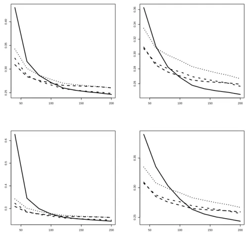
Based on the evaluation of mean squared errors, the graphs in Figure 1 show that the factor VAR model dominates at larger sample sizes in all designs, that is for AIC as well as BIC and for two as well as three factors. Unreported control experiments have shown that this is not true for FAVAR variants that do not explicitly include the predicted variable as an additional factor. In other words, the factor search is unable to locate the most important variable for forecasting, the target variable itself, as it concentrates on variance contributions. However, it is successful in adding factors to the list, while we do not have proof that this choice is optimal with regard to prediction.

In small samples, the univariate autoregression dominates but it loses ground as the sample size increases. Among the two bivariate VAR models, a clear ranking is recogniz- able. Model #3 with output and nominal interest rate achieves a more precise prediction for output than model #2 with output and inflation. This ranking is due to the structure of the DSGE model that assumes stronger links between output and the interest rate than between output and inflation.

Figure 1 restricts attention to single-step prediction. Results for longer horizons are very similar and are not reported. They are available upon request.

4.2 Weights in the combination forecasts

The univariate model is best for small samples, the FAVAR is best for large samples. Thus, one may expect that the FAVAR model receives a stronger weight in the encompassing-test

8

50 100 150 200

0.250.300.350.40

50 100 150 200

0.260.280.300.320.340.36

50 100 150 200

0.30.40.50.6

50 100 150 200

0.250.300.35

Figure 1: MSE for the four competing forecast models in single-step prediction. Solid curve stands for FAVAR, dashed for the univariate AR model, dotted and dash-dotted for bivariate VAR models. Left graphs for AIC search, right graphs for BIC search, top graphs for two factors FAVAR, bottom row for three factors.

9

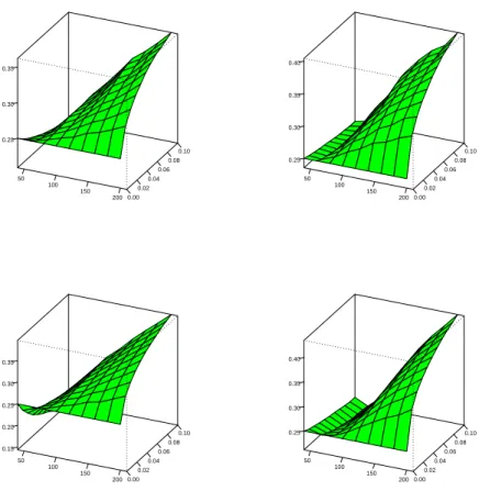
weighting procedure, as the samples get larger.¹ Figure 2 shows that this is indeed the case.

There are slight differences between the AIC and BIC search, as reaction is monotonic for AIC at all sample sizes. Note that even for BIC order selection the competing and less informative models outperform the FAVAR model in small samples with respect to the MSE criterion (see Figure 1). However, this behavior does not entail forecast encompassing any more, due to the heavily penalized and thus typically low lag orders.

50 100

150 200 0.00

0.02 0.04

0.06 0.08

0.10 0.25

0.30 0.35

50 100

150 200 0.00

0.02 0.04

0.06 0.08

0.10 0.25

0.30 0.35 0.40

50 100

150 200 0.00

0.02 0.04

0.06 0.08

0.10 0.15

0.20 0.25 0.30 0.35

50 100

150 200 0.00

0.02 0.04

0.06 0.08

0.10 0.25

0.30 0.35 0.40

Figure 2: Weights allotted to the FAVAR model in dependence of the sample size and of the significance level for the encompassing test in single-step prediction. Arrangement of graphs as in Figure 1.

As the significance level increases, weights diverge from the uniform pattern. We note, however, that even at 10% and N = 200 the weight allotted to the FAVAR model does not exceed around 40%. This value is an average over many replications with uniform weighting and comparatively few where weights of 1/3, of 1/2, or even of one are allotted to FAVAR.

1Ericsson (1992) showed that the null hypothesis of the forecast encompassing test is a sufficient con- dition for forecast MSE dominance.

10

When the prediction horizon grows, the main features of Figure 2 continue to hold, with one noteworthy exception. For larger samples, Figure 2 shows a smooth increase of the weight allotted to the FAVAR model with rising significance level. At larger horizons, this slope steepens, such that even at the 1% level a considerable weight is attained for FAVAR. This stronger discrimination among rival models affects the accuracy comparison to be reported in the next subsection.

4.3 Performance of test-based weighting

In order to evaluate the implications of the test-based method for forecasting, we use three criteria: the mean squared error (MSE), the mean absolute error (MAE), and the winning incidence. Generally, the MAE yields similar qualitative results as the MSE and we do not show the MAE results in detail.

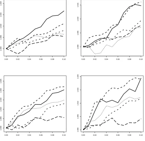
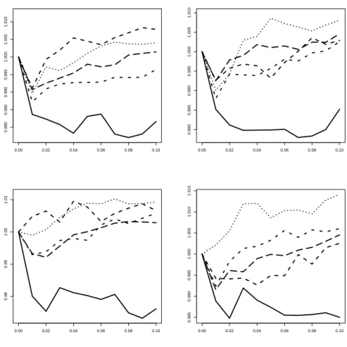
Figures 3 to 6 shows ratios of the MSE achieved by the test-based weighting relative to the benchmark of a uniformly weighted forecast, depending on the sample size. Values below one indicate an advantage for the test-based procedure. In order not to overload the graphs, they contain results for N ∈ {40,80,120,160,200} only, while all simulation results are available for N = 40 +k ∗20, k = 0, . . . ,8. The intermediate values always correspond to roughly interpolated curves, so little information is lost here.

For single-step prediction (see Figure 3), differences among models are small and remain in the range of 2% at the maximum values. In small samples, uniform weighting clearly outperforms the test-based weighting scheme. Performance is often monotonic in the sense that a looser significance level and thus a greater divergence from uniformity implies further deterioration. However, it is known from Figure 2 that these differences to uniformity are small. At larger samples, the differences among significance levels decrease, and there are several occasions where the test-based weighting achieves values below one and thus appears to be preferable. The AIC experiments are slightly more friendly to the test-based rules than the BIC experiments. In one case, there is a noteworthy non-monotonic reaction.

The qualitative results are robust if the mean absolute error (MAE) replaces the MSE as the prediction criterion. While the performance for two factors is indeed almost identical to the MSE evaluation, it is slightly less favorable to test-based weighting for three factors.

For brevity, these results are not shown in detail.

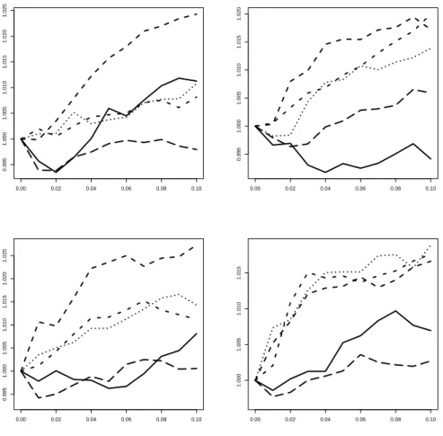
If the step size increases, the occurrence of ties among the procedures becomes less prominent. This, in turn, leads to a clearer separation with regard to the accuracy ensuing from prediction models. The weight allotted to the best model, in large samples the FAVAR model, increases.

The graphs for the case of two-step predictions, Figure 4, show that this stronger emphasis on the FAVAR model leads to an improvement in accuracy for the largest sample size N = 200 and for the smallest sample size N = 40, while no gains are recognizable for intermediate cases.

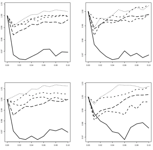
Extending the prediction horizon to three yields the graphs given as Figure 5. Test- based weighting dominates uniform weights at most sample sizes and specifications. The significance level of 1%, i.e. the sharpest level, is clearly supported over the looser levels

11

0.00 0.02 0.04 0.06 0.08 0.10

1.0001.0051.0101.0151.020

0.00 0.02 0.04 0.06 0.08 0.10

1.0001.0051.0101.015

0.00 0.02 0.04 0.06 0.08 0.10

1.0001.0051.0101.0151.0201.025

0.00 0.02 0.04 0.06 0.08 0.10

1.0001.0051.0101.0151.020

Figure 3: Ratios of test-based weighting MSE divided by the MSE from uniform weighting.

Ordering of graphs see Figure 1. Solid curve for N = 40, short dashes for N = 80, dotted curve forN = 120, dash-dotted forN = 160, long dashes forN = 200.

12

0.00 0.02 0.04 0.06 0.08 0.10

0.9951.0001.0051.0101.0151.0201.025

0.00 0.02 0.04 0.06 0.08 0.10

0.9951.0001.0051.0101.0151.020

0.00 0.02 0.04 0.06 0.08 0.10

0.9951.0001.0051.0101.0151.0201.025

0.00 0.02 0.04 0.06 0.08 0.10

1.0001.0051.0101.015

Figure 4: Ratios of test-based weighting MSE to MSE from uniform weighting in two-step prediction. Ordering of graphs see Figure 1. Solid curve for N = 40, short dashes for N = 80, dotted curve for N = 120, dash-dotted forN = 160, long dashes for N = 200.

13

0.00 0.02 0.04 0.06 0.08 0.10

0.9800.9850.9900.9951.0001.0051.010

0.00 0.02 0.04 0.06 0.08 0.10

0.9800.9850.9900.9951.0001.0051.010

0.00 0.02 0.04 0.06 0.08 0.10

0.980.991.001.01

0.00 0.02 0.04 0.06 0.08 0.10

0.9850.9900.9951.0001.0051.0101.015

Figure 5: Ratios of test-based weighting MSE to MSE from uniform weighting in three-step prediction. Ordering of graphs see Figure 1. Solid curve for N = 40, short dashes for N = 80, dotted curve for N = 120, dash-dotted forN = 160, long dashes for N = 200.

14

0.00 0.02 0.04 0.06 0.08 0.10

0.970.980.991.001.01

0.00 0.02 0.04 0.06 0.08 0.10

0.970.980.991.00

0.00 0.02 0.04 0.06 0.08 0.10

0.970.980.991.001.01

0.00 0.02 0.04 0.06 0.08 0.10

0.970.980.991.001.01

Figure 6: Ratios of test-based weighting MSE to MSE from uniform weighting in four-step prediction. Ordering of graphs see Figure 1. Solid curve for N = 40, short dashes for N = 80, dotted curve for N = 120, dash-dotted forN = 160, long dashes for N = 200.

15

for the encompassing test. These features are confirmed and slightly enhanced by the four- step predictions summarized in Figure 6. Here, test-based weighting dominates in all four variants for all sample sizes, with only one exception. Advantages for test-based weighting are most pronounced in the smallest and largest samples.

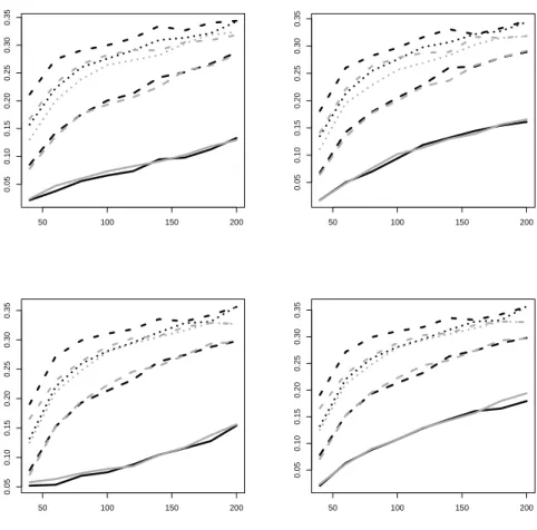
The criteria MAE and MSE are summary statistics, and they are based on moments of the error distributions. A lower MSE may be attained by a forecast that is actually worse in many replications but wins few of them at a sizeable margin. Therefore, we also consider the direct ranking of squared errors across significance levels. The incidence of a minimum among all levels could indicate which level is more likely to generate the best forecast. There are many ties among these significance levels, however, so we only report the direct comparison between the 1% test-based weighting and the uniform benchmark in more detail. Figure 7 shows the frequencies of each of these two models of generating the smaller prediction error.

50 100 150 200

0.050.100.150.200.250.300.35

50 100 150 200

0.050.100.150.200.250.300.35

50 100 150 200

0.050.100.150.200.250.300.35

50 100 150 200

0.050.100.150.200.250.300.35

Figure 7: Frequency of a smaller absolute forecast error due to uniform weighting (gray curves) or 1% test-based weighting (black curves). Forecasts at horizons one (solid), two (dashed), three (dotted), and four (dash-dotted). Ordering of graphs see Figure 1.

16

For one-step forecasts, Figure 7 clearly demonstrates that the differences in MSE re- ported above are due to comparatively few replications. Ties are many even for large samples (around 70%) and are the rule for small samples (around 90%). The direct com- parison is not generally favorable for the test-based scheme. Uniform weighting wins for some cases even at N = 200. On the other hand, the dominance of uniform weighting that follows from the MSE graphs is not replicated here, and test-based weighting appears competitive even for small samples.

In line with the MSE graphs, also the ‘winning frequency’ for the test-based scheme improves at larger forecast horizons. At two steps, the two schemes are comparable, with a slight advantage for the encompassing test, and at three and four steps the test-based procedure gains a sizeable margin. Also note that ties become less frequent and their frequency falls to around 30% at horizon four and larger samples.

In summary, at larger prediction horizons test-based weighting becomes increasingly attractive. At short horizons, the merits of test-based weighting are most pronounced for very small samples, where the accuracy of prediction is low, and at larger samples, where weighting becomes reliable. Unfortunately, many empirical samples may belong to the intermediate region, where the prediction horizon must exceed two in order to provide a clear support for weights based on the encompassing test.

17

5 Conclusion

Our forecast evaluations generally confirm the traded wisdom in the forecasting literature that uniform weighting of rival model forecasts is difficult to beat in typical forecasting situations. Large sample sizes are needed to reliably eliminate inferior rival models from forecasting combinations. In many situations of empirical relevance, the information con- tained in slightly worse predictions as marked by individual MSE performance may still be helpful for increasing the precision of the combination.

Forecast-encompassing tests imply a reasonable weighting of individual models in our experiments. Univariate models yield the best forecasts in small samples, and sophisticated higher-dimensional models receive a small weight. With increasing sample size, our exper- iments clearly show that the factor-augmented VAR achieves the best predictive accuracy and thus it receives the largest weights in test-based combinations. The benefits with respect to an optimized combination forecast, however, turn out to be more difficult to exploit. At the one-step horizon, the test-based combination forecast fails to show a clear dominance over a simple uniform weighting procedure even in large samples. Only at hori- zons of three and beyond does the dominance of test-based weighting become convincing.

A noteworthy general result is that, for the encompassing test, the sharpest significance level of 1% yields the best results.

References

[1] Adolfson, M, Lind´e, J, Villani, M. 2007. Forecasting Performance of an Open Economy DSGE Model. Econometric Reviews 26: 289–328.

[2] An, S, Schorfheide, F. 2007. Bayesian Analysis of DSGE Models.Econometric Reviews 26: 113–172.

[3] Bai, J, Ng, S. 2002. Determining the Number of Factors in Approximate Factor Mod- els. Econometrica 70, 191–221.

[4] Bates, JM, Granger, CWJ. 1969. The combination of forecasts. Operations Research Quarterly20: 451–468.

[5] Blanchard, OJ, Kahn, CM. 1980. The Solution of Linear Difference Models under Rational Expectations. Econometrica 48: 1305–1311.

[6] Calvo, GA. 1983. Staggered prices in a utility-maximizing framework.Journal of Mon- etary Economics 12: 383–398.

[7] Clements, M, Hendry, DF. 1998. Forecasting economic time series. Cambridge Uni- versity Press.

18

[8] Costantini, M, Kunst, RM. 2009. Combining forecasts based on multiple encompass- ing tests in a macroeconomic core system. Economics Series No. 243, Institute for Advanced Studies, Vienna.

[9] Costantini, M, Pappalardo, C. 2010. Hierarchical procedure for the combination of forecasts. International Journal of Forecasting, forthcoming.

[10] de Menezes, L, Bunn, DW. 1993. Diagnostic Tracking and Model Specification in Combined Forecast of U.K. Inflation. Journal of Forecasting 12: 559–572.

[11] Ericsson, NR. 1992. Parameter constancy, mean square forecast errors, and measuring forecast performance: An exposition, extensions, and illustration. Journal of Policy Modeling 14: 465–495.

[12] Harvey, D. I., Leybourne, S., Newbold, P. 1998. Tests for forecast encompassing.

Journal of Business and Economic Statistics,16: 254–259.

[13] Harvey, D.I., Newbold, P. 2000. Tests for Multiple Forecast Encompassing.Journal of Applied Econometrics 15: 471–482.

[14] Kascha, C, Mertens, K. 2009. Business cycle analysis and VARMA models. Journal of Economic Dynamics & Control 33: 267–282.

[15] L¨utkepohl, H. 2005. New Introduction to Multiple Time Series. Springer.

[16] Ravenna, F. 2007. Vector autoregressions and reduced form representations of DSGE models. Journal of Monetary Economics 54: 2048–2064.

[17] Schmitt-Groh´e, S, Uribe, M. 2004. Solving dynamic general equilibrium models using a second-order approximation to the policy function. Journal of Economic Dynamics

& Control 28: 755–775.

[18] Smets, F, Wouters, R. 2003. An Estimated Dynamic Stochastic General Equilibrium Model of the Euro Area.Journal of the European Economic Association1: 1123–1175.

[19] Smets, F, Wouters, R. 2004. Forecasting with a Bayesian DSGE Model: An Applica- tion to the Euro Area. Journal of Common Market Studies 42: 841–867.

[20] Stock, JH, Watson, MW. 1998. Diffusion indexes. Working paper No. 6702, NBER.

[21] Stock, JH, Watson, MW. 2002. Macroeconomic forecasting using diffusion indices.

Journal of Business & Economic Statistics 20, 147–162.

[22] Timmermann, A. 2006. Forecast combinations, in Elliott, G, Granger, CWJ, and Timmermann, A. (ed.), Handbook of Economic Forecasting, Elsevier.

19

Authors: Mauro Costantini, Ulrich Gunter, Robert M. Kunst

Title: Forecast Combination Based on Multiple Encompassing Tests in a Macroeconomic DSGE System

Reihe Ökonomie / Economics Series 251

Editor: Robert M. Kunst (Econometrics)

Associate Editors: Walter Fisher (Macroeconomics), Klaus Ritzberger (Microeconomics)

ISSN: 1605-7996

© 2010 by the Department of Economics and Finance, Institute for Advanced Studies (IHS),

Stumpergasse 56, A-1060 Vienna   +43 1 59991-0  Fax +43 1 59991-555  http://www.ihs.ac.at

ISSN: 1605-7996