M ULTIPLE REGRESSION : W HY ?

M ULTIPLE REGRESSION : W HY ?

Werner A. Stahel Seminar f¨ur Statistik, ETH CH-8092 Z¨urich, Switzerland

October 2006

Abstract

The differences between fitting a single multiple regression with several explanatory variables and the re- spective number of simple regression fits are illustrated with a practical example from public health.

1 Introduction

Regression studies relationships between a target or response variable and one or more explanatory vari- ables. The case of a single explanatory variable, leading to simple regression, is easy to understand at least intuitively, since the scatterplot “tells the story”. When there are two or more explanatory variables, a naive approach is to fit a simple regression for each variable in turn. It is a basic fact that this can give very different results from fitting a multiple regression with all explanatory variables – if correlations occur among explanatory variables, as is typical for all observational studies. (In experiments, the problem is avoided by the experimental design.)

In this note, we use a practical example from public health to illustrate such differences. The dataset was collected for a study in 2002 (Gesundheitsstudie 2002) by the Swiss Statistical Office. Questionaires were filled in by 16,141 persons. Julie Marc and Laura Vinckenbosch developped multiple regression models for a target variable they called happyness (Zufriedenheit), among others, in an unpublished semester study in 2004. In fact, happyness was calculated summing over different items asking for different aspects of this theme. They also selected three personal conditions (age, body mass index, income) and 30 questionaire items as potential explanatory variables. A rough description of the variables is given in Table 1. For the purpose of this study, 1436 persons were selected randomly.

In the following section, we give a very brief introduction to simple and multiple regression, including the backward elimination procedure to obtain a reduced multiple regression model. Many textbooks contain an adequate treatment of these topics, for example Draper and Smith (1998), Ryan (1997), Chatterjee and Price (2000), and Weisberg (1990).

label meaning (codes) age age in years ag40 age, censored at 40

inc income in CHF; incl: log transformed bmi body mass index; bmil: log transformed vio violence index (1-4)

SupportThere exists someone who (1-5) ssck helps when confined to bed

slis listens when I want to speak out scrs stands by in crises

sapp expresses appreciation shug hugs me

disturbancein the flat by (codes 0-1) ntrf noise from car traffic

ntrn noise from railway lines nair noise from air traffic nind noise from industry

npeo noise from people or children ptrf traffic pollution

pind industrial pollution or foul odor pagr agricultural immissions dist other disturbances nodi no disturbance

Fitness

fgen sweat once a week because of physical activities (0-1) ftrn gymnastics, fitness or sports activities (0-1)

fdfr days a week with ... activities in free time (0-7) fdwo days a week with ... activities at work (0-7) fsuf sufficient activity (personal judgement) (0-1)

Miscellaneous

hlb hours of housekeeping work per week / 10 chi having children (young or adult) (0-1)

fri there is a person to talk about personal problems (0-2) hlp offering unpaid help regularly (0-1)

rel religious activities (0-7) clb being member of a club (0-1) pet pet in the household (0-1) hiv having had a HIV test (0-1)

Table 1: Explanatory variables used in the example

2 Models

Simple linear regressionis based on the following model relating the target variable

Y

to the explanatory variable

X

^(j):

Y

i

= α + βX

_i^(j)

+ E

i

,

where

Y

i is the value of the response variable for person

i

,

X

_i^(j) is the value of the explanatory variable under consideration,

E

iis the unexplained random deviation of

Y

ifrom the “model value”, and

α

and

β

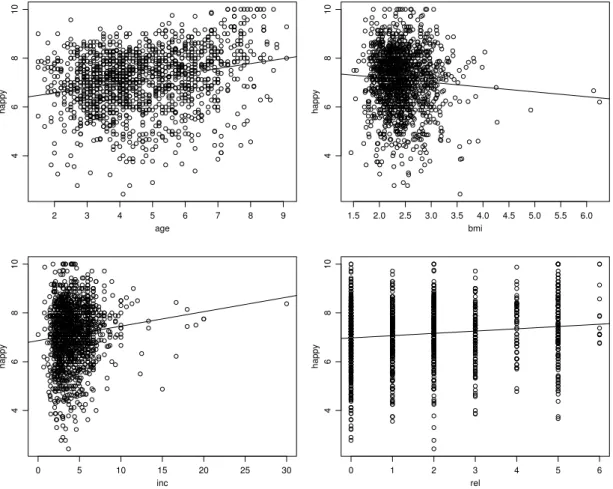
are the intercept and the slope of the straight line characterizing the model.

Figure 1 shows the scatterplots illustrating the simple regressions for four explanatory variables.

2 3 4 5 6 7 8 9

46810

age

happy

1.5 2.0 2.5 3.0 3.5 4.0 4.5 5.0 5.5 6.0

46810

bmi

happy

0 5 10 15 20 25 30

46810

inc

happy

0 1 2 3 4 5 6

46810

rel

happy

Figure 1: Four simple regressions: Scatterplots of happyness against age, body mass index, income, and religious activities with best fitting straight lines

It is good practice to use some explanatory variables in atransformed formin the model. This is the case for income and body mass index (bmi), which are transformed by taking logarithms, following the principle of applying the so-called first aid transformation as introduced by John Tukey. The plots also suggest that the distribution of the random deviations is skewed to the right, due to the “roof effect” of the maximum score value of 10 for happyness. We therefore square the response variable. Furthermore, plotting residuals of a multiple model against explanatory variables suggested that the influence of age was not linear. Censoring

regression to be introduced. Then, the model reads

Y

i

= α

j

+ β

_j^∗

X

_i^(j)

+ E

_i^(j)

.

Themultiple regression modelincludes all explanatory variables in one single model,

Y

i

= β

₀

+ β

₁

X

_i⁽¹⁾

+ β

₂

X

_i⁽²⁾

+ ... + β

m

X

_i^(m)

+ E

i

.

The model describes the idea that the effects of the different variables, measured by

β

j

X

_i^(j), add to result in an expected value for

Y

i. Thecoefficient

β

jexpresses by what amount

Y

iwould increase if the explanatory variable

X

_i^(j) was increased by one unit and all the other variables were kept constant (which may be impossible in some situations). The coefficients

β

_j^∗of the simple regressions, in contrast, measure the effect of increasing the respective explanatory variable

X

^(j)by one unit while all the others change according to their correlations with

X

^(j). Therefore, the two types of coefficients measure different quantities if there are correlations among the explanatory variables.

Remark. If the explanatory variables are uncorrelated, then the coefficients have the same interpretations, and the advantage of a multiple regression over the collection of simple ones consists just in an increased precision of estimation. Uncorrelated explanatory variables typically occur in properly designed experiments.

Multiple regression results are somewhat difficult to interpret if someexplanatory variables are strongly correlated. It may be then sufficient to include one of them in the model. Since each of them can be dropped from the model without deteriorating the fit noticeably, both appear unimportant if judged by statistical sig- nificance of their coefficients, even if dropping both clearly deteriorates the model. Similar considerations hold for more complicated relations between explanatory variables, giving rise to a so-calledcollinearity problem.

To overcome this difficulty, it is common toreduce the modelincluding all explanatory variables in a step- wise fashion by eliminating in each step the variable which is least significant, until an appropriate criterion suggests to stop this process. The most popular criterion nowadays is Akaike’s Information Criterion (AIC) or a version of it. Traditionally, the process was stopped when all variables in the reduced model were for- mally significant (at the 5% level). It is important to be aware that such significance cannot be interpreted in the classical way of hypothesis testing with a given probability of an “error of the first kind” (rejecting a true hypothesis

β

j

= 0

), due to the fact that many potential hypotheses are tested. See the literature on regression for a more detailed description of this issue, called the “problem of multiplicity”. Note that AIC is usually more liberal than the latter rule, that is, it often leaves some variables in the model which have a p-value above 5%. Here, we use the reduced model according to the “significance stopping rule”.

In the next section, we compare the coefficients obtained from the simple regressions with those of the full and the reduced multiple regression model. The common, sloppy questions are: “Does variable

X

^(j)

influence the response

Y

? Is the influence statistically significant? Is it positive or negative?

3 Results

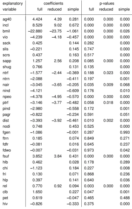
Table 2 presents estimated coefficients for the full and reduced multiple regression model and for the simple models, followed by respective p-values. (A p-value below 5% means that the corresponding coefficient is significantly different from zero –

X

^(j) is then said to have a significant influence on

Y

.) The gaps in the column for the reduced model correspond to the variables that have been dropped by the backward elimination procedure described above. According to the reduced model, these variables have no influence on the response.

Comparing the p-values of the full and reduced multiple model shows that all the dropped variables have been insignificant in the full model, with the exception of “clb” (club membership), which was barely significant. On the other hand, three variables – “sapp,” “ntrf,” and “ptrf” – turned from insignificant to significant. In the full model, there are other variables, correlated with these, that somehow competed with them for significance and are eliminated in the procedure. In some instances, one of them might replace one of the three that were kept without deteriorating the model. A more complete discussion would include other models judged as being of almost the same quality, obtained from examining all possible models (“all subsets”).

The principal contrast is between the p-values and coefficients of the reduced model and the simple regres- sions. Many variables appear highly significant when judged by simple regression, but are absent from the reduced multiple model and insignificant in the full model. As explained above, such effects usually occur if explanatory variables are correlated. The correlation matrix is therefore given in the Appendix for the sake of reference.

Let us comment on some salient points:

•

All variables included in the reduced model show significant p-values for the simple regression coeffi- cient, too – with the minor exception of “nair”.

•

The “support” items “ssck,” “slis,” “scrs,” and “shug” are not included in the reduced model, but are highly significant according to simple regression. It seems that the remaining support variable “sapp”

suffices to describe the influence of support on happyness. The correlations among pairs of these variables all exceed or equal 0.49 (see Table 3), which supports the interpretation that these variables are so closely related that they can replace each other. Appreciation “sapp” appears to be the most relevant variable – but note that such an interpretation cannot be labeled as statistically proven. The conclusion that all other support does not influence happyness would be misleading.

•

Having children has a positive influence on happyness if judged by simple regression. The effect disappears for the multiple model. In the full model, a negative influence is estimated – but clearly insignificant.

•

An HIV test is related to a lack of happyness as determined by simple regression. Again, no such effect is suggested by the multiple models. In fact, if “ag40” and “incl” are included in a model along with “hiv”, then the latter becomes insignificant. Age and income are both negatively correlated with

“hiv”, but have a positive influence on happyness.

•

Several variables which might be expected to contribute to happyness do not show any significance in any model. These include household labor (hlb), having a friend (fri), helping others (hlp), and having a pet in the household (pet).

explanatory coefficients p-values

variable full reduced simple full reduced simple

ag40 4.424 4.39 0.281 0.000 0.000 0.000

incl 8.529 9.02 0.672 0.000 0.000 0.000

bmil –22.880 –23.75 –1.061 0.000 0.000 0.026

vio –4.239 –4.18 –0.457 0.000 0.000 0.000

ssck 0.425 0.144 0.282 0.000

slis –0.221 0.145 0.747 0.000

scrs 0.437 0.163 0.517 0.000

sapp 1.257 2.56 0.208 0.085 0.000 0.000

shug 0.766 0.131 0.135 0.000

ntrf –1.577 –2.44 –0.369 0.188 0.023 0.000

ntrn –2.088 –0.411 0.197 0.001

nair –3.045 –3.65 –0.205 0.035 0.009 0.068

nind –4.121 –0.609 0.176 0.010

npeo –4.378 –4.95 –0.570 0.000 0.000 0.000 ptrf –3.146 –3.77 –0.482 0.058 0.018 0.000

pind –2.980 –0.558 0.172 0.001

pagr –0.822 –0.234 0.591 0.051

dist –3.393 –3.92 –0.461 0.010 0.002 0.000

nodi 0.748 0.453 0.525 0.000

fgen –1.086 –0.001 0.287 0.993

ftrn 0.185 0.074 0.849 0.271

fdfr –0.081 0.016 0.645 0.237

fdwo –0.007 –0.031 0.973 0.042

fsuf 3.852 3.84 0.431 0.000 0.000 0.000

hlb 0.462 0.028 0.178 0.289

chi –1.123 0.184 0.227 0.008

fri 0.130 0.071 0.868 0.236

hlp 0.397 0.141 0.640 0.036

rel 0.770 0.92 0.094 0.003 0.000 0.000

clb 1.650 0.227 0.047 0.001

pet 0.619 –0.047 0.465 0.488

hiv –0.826 –0.333 0.375 0.000

Table 2: Results of fitting a full multiple regression, a reduced model, and simple regression models

4 Conclusions

As mentioned above, the question often asked in connection with a response and several potential explana- tory variables is: “Which explanatory variables have an influence on the response?”

Even though this question appears to be reasonably clear, there is no unique, correct answer. The “influence”

depends on other variables in the model. If the question asks for a specific influence that cannot be taken up by other observed explanatory variables, then the full multiple regression analysis gives an answer. It is, however, important to keep in mind that many hypotheses are tested on the same dataset, and the problem of multiplicity limits the interpretation of the p-values for testing for zero coefficients

β

j.

The ultimate purpose of scientific studies often focuses on causal relations. One would like to single out all causes for the resulting values of the response. This is only possible in designed experiments, where the difficulties discussed in this note are avoided by making explanatory variables uncorrelated (and nominal variables or factors, balanced). Nevertheless, a significant coefficient in a multiple regression model is the strongest hint at causal relations that can be obtained in an observational study like the example discussed here. Such a significant coefficient

β

jcannot be due to an indirect effect of the following nature: Suppose that there is a further variable having a causal relationship with both the considered variable

X

^(j)and the response

Y

. This would lead to a correlation between

X

^(j) and

Y

, potentially resulting in a significant coefficient

β

j. If the common cause is also included in the model, its coefficient would show its influence, and the coefficient

β

_jwould not be affected by this indirect influence.

For simple regression, such indirect effects are very likely. An example is the variable hiv, which becomes insignificant if age and income are included in the model.

Summarizing, interpretation of regression models for observational studies is a delicate task. Multiple re- gression models may often lead to deeper conclusions than a collection of simple regression analyses.

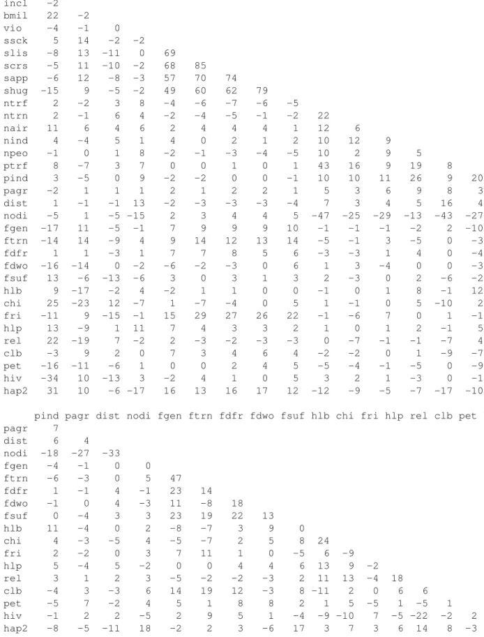
Appendix: Correlation among variables

Table 3 exhibits simple Pearson correlations. They may help to interpret differences between simple and multiple regression coefficients.

References

Chatterjee, S. and Price, B. (2000).Regression Analysis By Example, 3rd edn, Wiley, N.Y.

Draper, N. and Smith, H. (1998).Applied Regression Analysis, 3rd edn, Wiley, N.Y.

Ryan, T. P. (1997).Modern Regression Methods, Series in Probability and Statistics, Wiley, N.Y. includes disk Weisberg, S. (1990).Applied Linear Regression, 2nd edn, Wiley, N.Y.

ag40 incl bmil vio ssck slis scrs sapp shug ntrf ntrn nair nind npeo ptrf incl -2

bmil 22 -2

vio -4 -1 0

ssck 5 14 -2 -2 slis -8 13 -11 0 69 scrs -5 11 -10 -2 68 85 sapp -6 12 -8 -3 57 70 74 shug -15 9 -5 -2 49 60 62 79

ntrf 2 -2 3 8 -4 -6 -7 -6 -5

ntrn 2 -1 6 4 -2 -4 -5 -1 -2 22

nair 11 6 4 6 2 4 4 4 1 12 6

nind 4 -4 5 1 4 0 2 1 2 10 12 9

npeo -1 0 1 8 -2 -1 -3 -4 -5 10 2 9 5

ptrf 8 -7 3 7 0 0 1 0 1 43 16 9 19 8

pind 3 -5 0 9 -2 -2 0 0 -1 10 10 11 26 9 20

pagr -2 1 1 1 2 1 2 2 1 5 3 6 9 8 3

dist 1 -1 -1 13 -2 -3 -3 -3 -4 7 3 4 5 16 4

nodi -5 1 -5 -15 2 3 4 4 5 -47 -25 -29 -13 -43 -27

fgen -17 11 -5 -1 7 9 9 9 10 -1 -1 -1 -2 2 -10

ftrn -14 14 -9 4 9 14 12 13 14 -5 -1 3 -5 0 -3

fdfr 1 1 -3 1 7 7 8 5 6 -3 -3 1 4 0 -4

fdwo -16 -14 0 -2 -6 -2 -3 0 6 1 3 -4 0 0 -3

fsuf 13 -6 -13 -6 3 0 3 1 3 2 -3 0 2 -6 -2

hlb 9 -17 -2 4 -2 1 1 0 0 -1 0 1 8 -1 12

chi 25 -23 12 -7 1 -7 -4 0 5 1 -1 0 5 -10 2

fri -11 9 -15 -1 15 29 27 26 22 -1 -6 7 0 1 -1

hlp 13 -9 1 11 7 4 3 3 2 1 0 1 2 -1 5

rel 22 -19 7 -2 2 -3 -2 -3 -3 0 -7 -1 -1 -7 4

clb -3 9 2 0 7 3 4 6 4 -2 -2 0 1 -9 -7

pet -16 -11 -6 1 0 0 2 4 5 -5 -4 -1 -5 0 -9

hiv -34 10 -13 3 -2 4 1 0 5 3 2 1 -3 0 -1

hap2 31 10 -6 -17 16 13 16 17 12 -12 -9 -5 -7 -17 -10 pind pagr dist nodi fgen ftrn fdfr fdwo fsuf hlb chi fri hlp rel clb pet hiv pagr 7

dist 6 4

nodi -18 -27 -33

fgen -4 -1 0 0

ftrn -6 -3 0 5 47

fdfr 1 -1 4 -1 23 14

fdwo -1 0 4 -3 11 -8 18

fsuf 0 -4 3 3 23 19 22 13

hlb 11 -4 0 2 -8 -7 3 9 0

chi 4 -3 -5 4 -5 -7 2 5 8 24

fri 2 -2 0 3 7 11 1 0 -5 6 -9

hlp 5 -4 5 -2 0 0 4 4 6 13 9 -2

rel 3 1 2 3 -5 -2 -2 -3 2 11 13 -4 18

clb -4 3 -3 6 14 19 12 -3 8 -11 2 0 6 6

pet -5 7 -2 4 5 1 8 8 2 1 5 -5 1 -5 1

hiv -1 2 2 -5 2 9 5 1 -4 -9 -10 7 -5 -22 -2 2

hap2 -8 -5 -11 18 -2 2 3 -6 17 3 7 3 6 14 8 -3 -13

Table 3: Correlations among variables, mulitplied by 100