The Monash Simple Climate Model

The Monash Simple Climate Model

1

Experiments (MSCM-DB v1.0): An

2

interactive database of mean climate,

3

climate change and scenario

4

simulations

5

By Dietmar Dommenget^1*, Kerry Nice^1,4, Tobias Bayr², Dieter Kasang³, Christian 6

Stassen¹ and Mike Rezny¹ 7

8

*: corresponding author; dietmar.dommenget@monash.edu 9

1: Monash University, School of Earth, Atmosphere and Environment, Clayton, Victoria 10

3800, Australia.

11

2: GEMOAR Helmholtz Centre for Ocean Research, Düsternbrooker Weg 20, 24105 Kiel, 12

Germany 13

3: DKRZ, Hamburg, Germany 14

4: Transport, Health, and Urban Design Hub, Faculty of Architecture, Building, and 15

Planning, University of Melbourne, Victoria 3010, Australia 16 17

submitted the Geoscientific Model Development, 8 March 2018 18

19

Abstract 20

This study introduces the Monash Simple Climate Model (MSCM) experiment 21 database. The model simulations are based on the Globally Resolved Energy 22

Balance (GREB) model. They provide a basis to study three different aspects of 23

climate model simulations: (1) understanding the processes that control the 24

mean climate, (2) the response of the climate to a doubling of the CO2

25

concentration, and (3) scenarios of external CO2 concentration and solar 26

radiation forcings. A series of sensitivity experiments in which elements of the 27

climate system are turned off in various combinations are used to address (1) 28

and (2). This database currently provides more than 1,300 experiments and has 29

an online web interface for fast analysis of the experiments and for open access 30

to the data. We briefly outline the design of all experiments, give a discussion of 31

some results, and put the findings into the context of previously published 32

results from similar experiments. We briefly discuss the quality and limitations 33

of the MSCM experiments and also give an outlook on possible further 34

developments. The GREB model simulation of the mean climate processes is 35

quite realistic, but does have uncertainties in the order of 20-30%. The GREB 36

model without flux corrections has a root mean square error in mean state of 37

about 10^°C, which is larger than those of general circulation models (2^°C).

38

However, the MSCM experiments show good agreement to previously published 39

studies. Although GREB is a very simple model, it delivers good first-order 40

estimates, is very fast, highly accessible, and can be used to quickly try many 41

different sensitivity experiments or scenarios.

42 43

1. Introduction

44

Our understanding of the dynamics of the climate system and climate changes is 45

strongly linked to the analysis of model simulations of the climate system using a 46

range of climate models that vary in complexity and sophistication. Climate 47

model simulations help us to predict future climate changes and they help us 48

gain a better understand of the dynamics of this complex system.

49

State-of-the-art climate models, such as used in the Coupled Model Inter- 50

comparison Project (CMIP; Taylor et al. 2012), are highly complex simulations 51

that require significant amounts of computing resources and time. Such model 52

simulations require a significant amount of preparation. The development of 53

idealized experiments that would help in the understanding and modelling of 54

climate system processes are often difficult to realize with the complex CMIP- 55

type climate models. In this context, simplified climate models are useful, as they 56

provide a fast first guess that help to inform more complex models. They also 57

help in understanding the interactions in the complex system.

58

In this article, we introduce the Monash Simple Climate Model (MSCM) database 59

(version: MSCM-DB v1.0). The MSCM is an interactive website 60 (http://mscm.dkrz.de, Germany and http://monash.edu/research/simple- 61

climate-model, Australia) and database that provide access to a series of more 62 than 1,300 experiments with the Globally Resolved Energy Balance (GREB) 63

model [Dommenget and Floter 2011; here after referred to as DF11]. The GREB 64

model was primarily developed to conceptually understand the physical 65

processes that control the global warming pattern in response to an increase in 66

CO2 concentration. It therefore centres around the surface temperature (Tsurf) 67

tendency equation and simulates only the processes needed for resolving the 68

global warming pattern.

69

Simplified climate models, such as Earth System Models of Intermediate 70

Complexity (EMICs), often aim at reducing the complexity to increase the 71

computation speed and therefore allow faster model simulations (e.g. CLIMBER 72

[Petoukhov et al. 2000], UVic [Weaver et al. 2001], FAMOUS [A] or LOVECLIM 73

[Goosse et al. 2010]). These EMICs are very similar in structure to state-of-the- 74

art Coupled General Circulation Models (CGCMs), following the approach of 75

simulating the geophysical fluid dynamics. The GREB model differs, in that it 76

follows an energy balance approach and does not simulate the geophysical fluid 77

dynamics of the atmosphere. It is therefore a climate model that does not include 78

weather dynamics, but focusses on the long term mean climate and its response 79

to external boundary changes.

80

The purpose of the MSCM database for research studies are the following:

81 82

• First Guess: The MSCM provides first guesses for how the climate may 83 change in idealized or realistic experiments. The MSCM experiments can 84

be used to test ideas before implementing and testing them in more 85 detailed CGCM simulations.

86

• Null Hypothesis: The simplicity of the GREB model provides a good null 87 hypothesis for understanding the climate system. Because it does not 88

simulate weather dynamics or circulation changes of neither large nor 89

small scale it provides the null hypothesis of a climate as a pure energy 90

balance problem.

91

• Conceptual understanding: The simplicity of the GREB model helps to 92

better understand the interactions in the complex climate and, therefore, 93

helps to formulate simple conceptual models for climate interactions.

94

• Education: Studying the results of the MSCM helps to understand the 95

interactions that control the mean state climate and its regional and 96

seasonal differences. It helps to understand how the climate will respond 97

to external forcings in a first-order approximation.

98 99

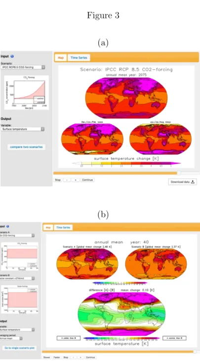
The MSCM provides interfaces for fast analysis of the experiments and selection 100

of the data (see Figs. 1-3). It is designed for teaching and outreach purposes, but 101

also provides a useful tool for researchers. The focus in this study will be on 102

describing the research aspects of the MSCM, whereas the teaching aspects of it 103

will not be discussed. The MSCM experiments focus on three different aspects of 104

climate model simulations: (1) understanding the processes that control the 105

mean climate, (2) the response of the climate to a doubling of the CO2

106

concentration, and (3) scenarios of external CO2 concentration and solar 107

radiation forcings. We will provide a short outline of the design of all 108

experiments, give a brief discussion of some results, and put the findings into 109

context of previously published literature results from similar experiments.

110

The DF11 study focussed primarily on the development of the model equations 111

and the discussion of the response pattern to an increase in CO2 concentration.

112

This study here will give a more detailed discussion on the performance of the 113

GREB model on simulation of the mean state climate.

114

The paper is organized as follows: The following section describes the GREB 115

model, the experiment designs, the MSCM interface, and the input data used. A 116

short analysis of the experiments is given in section 3. This section will mostly 117

focus on the GREB model performance in comparison to observations and 118

previously published simulations in the literature, but it will also give some 119

indications of the findings in the model experiments and the limitations of the 120

GREB model. The final section will give a short summary and outlook for 121

potential future developments and analysis.

122

2. Model and experiment descriptions

123

The GREB model is the underlying modelling tool for the MSCM interface. The 124

development of the model and all equations have been presented in DF11. The 125

model is simulating the global climate on a horizontal grid of 3.75^o longitude x 126

3.75^o latitude and in three vertical layers: surface, atmosphere and subsurface 127

ocean. It simulates the main physical processes that control the surface 128

temperature tendencies: solar (short-wave) and thermal (long-wave) radiation, 129

the hydrological cycle (including evaporation, moisture transport and 130

precipitation), horizontal transport of heat and heat uptake in the subsurface 131

ocean. Atmospheric circulation and cloud cover are seasonally prescribed 132

boundary condition, and state-independent flux corrections are used to keep the 133

GREB model close to the observed mean climate. Thus, the GREB model does not 134

simulate the atmospheric or ocean circulation and is therefore conceptually very 135

different from CGCM simulations.

136

The model does simulate important climate feedbacks such as the water vapour 137

and ice-albedo feedback, but an important limitation of the GREB model is that 138

the response to external forcings or model parameter perturbations do not 139

involve circulation or cloud feedbacks, which are relevant in CGCM simulations 140

[Bony et al. 2006].

141

Input climatologies (e.g. Tsurf or atmospheric humidty) for the GREB model are 142

taken from the NCEP reanalysis data from 1950-2008 [Kalnay et al. 1996], cloud 143

cover climatology from the ISCCP project [Rossow and Schiffer 1991], ocean 144

mixed layer depth climatology from Lorbacher et al. [2006], and topographic 145

data was taken from ECHAM5 atmosphere model [Roeckner et al. 2003].

146

GREB does not have any internal (natural) variability since daily weather 147

systems are not simulated. Subsequently, the control climate or response to 148 external forcings can be estimated from one single year. The primary advantage 149

of the GREB model in the context of this study is its simplicity, speed, and low 150

computational cost. A one year GREB model simulation can be done on a 151

standard PC computer in about 1 s (about 100,000 simulated years per day). It 152

can do simulations of the global climate much faster than any state-of-the-art 153

climate model and is therefore a good first guess approach to test ideas before 154

they are applied to more complex CGCMs. A further advantage is the lag of 155

internal variability which allows the detection of a response to external forcing 156

much more easily.

157

a. Experiments for the mean climate deconstruction 158

The conceptual deconstruction of the GREB model to understand the interactions 159

in the climate system that lead to the mean climate characteristics is done by 160

defining 11 processes (switches; see Fig. 1). For each of these switches, a term in 161

the model equations is set to zero or altered if the switch is “OFF”. The processes 162

and how they affect the model equations are briefly listed below (with a short 163

summary in Table 1). The model equations relevant for the experiments in this 164

study are briefly restated in the appendix section A1 for the purpose of 165

explaining each experimental setup in the MSCM.

166 167 168

Ice-albedo: The surface albedo (𝛼_"#$%) and the heat capacity over ocean points 169

(𝛾_"#$%) are influenced by snow and sea ice cover. In the GREB model these are a 170

direct function of Tsurf. When the Ice-albedo switch is OFF the surface albedo of 171

all points is constant (0.1) and, for ocean points, 𝛾_"#$% follows the prescribed 172

ocean mixed layer depth independent of Tsurf (i.e. no ice-covered ocean).

173 174

Clouds: The cloud cover, CLD, influences the amount of solar radiation absorbed 175

at the surface (𝛼_'()#*" in eq. [A5]) and the emissivity of the atmospheric 176

layer, 𝜀_-./)", for thermal radiation (eq. [A8]). When the Clouds switch is OFF, the 177 cloud cover is set to zero.

178 179

Oceans: The ocean in the GREB simulates subsurface heat storage with the 180

surface mixed layer (~upper 50-100m). When the ocean switch is OFF, the Focean

181

term in eq. [A1] is set to zero, eq. [A3] is set to zero and the heat capacity off all 182

ocean points is set to that of land points.

183 184

Atmosphere: The atmosphere in the GREB model simulates a number of 185

processes: The hydrological cycle, horizontal transport of heat, thermal 186

radiation, and sensible heat exchange with the surface. When the atmosphere 187

switch is OFF, eq. [A2] and [A4] are set to zero, the heat flux terms, Fsense and 188

Flatent in eq. [A1] are set to zero and the downward atmospheric thermal 189

radiation term in eq. [A6] is set to zero.

190 191

Diffusion of Heat: The atmosphere transports heat by isotropic diffusion (4^th 192

term in eq. [A2]). When this process is switched OFF, the term is set to zero.

193 194

Advection of Heat: The atmosphere transports heat by advection following the 195

mean wind field, 𝑢 (5^th term in eq. [A2]). When this process is switched OFF, the 196 term is set to zero.

197 198

CO2: The CO2 concentration affects the emissivity of the atmosphere, 𝜀_-./)" (eq.

199

[A9]). When this process is switched OFF, the CO2 concentration is set to zero.

200 201

Hydrological cycle: The hydrological cycle in the GREB model simulates the 202

evaporation, precipitation, and transport of atmospheric water vapour. It further 203

simulates latent heat cooling at the surface and heating in the atmosphere. When 204

the hydrological cycle is switched OFF, eq. [A4] is set to zero, the heat flux term 205

Flatent in eq. [A1] is set to zero, and 𝑣𝑖𝑤𝑣_-./)" in eq. [A9] is set to zero.

206

Subsequently, atmospheric humidity is zero.

207

It needs to be noted here, that the atmospheric emissivity in the log-function 208

parameterization of eq. [A9] can become negative, if the hydrological cycle, cloud 209

cover and CO2 concentration are switched OFF (set to zero). This marks an 210

unphysical range of the GREB emissivity function and we will discuss the 211

limitations of the GREB model in these experiments in Section 3b.

212 213

Diffusion of Water Vapour: The atmosphere transports water vapour by 214

isotropic diffusion (3^rd term in eq. [A4]). When this process is switched OFF, the 215

term is set to zero.

216

217 Advection of Water Vapour: The atmosphere transports heat by advection 218

following the mean wind field, 𝑢 (5^th term in eq. [A2]). When this process is 219

switched OFF, the term is set to zero.

220 221

Model Corrections: The model correction terms in eqs. [A1, A3 and A4]

222

artificially force the mean 𝑇_"#$%, 𝑇_-./)", and 𝑞_-6$ climate to be as observed. When 223

the model correction is switched OFF, the three terms are set to zero. This will 224

allow the GREB model to be studied without any artificial corrections and 225

therefore help to evaluate the GREB model equations’ skill in simulating the 226

climate dynamics.

227

It should be noted here that the model correction terms in the GREB model have 228

been introduced to study the response to doubling of the CO2 concentration for 229

the current climate, which is a relative small perturbation if compared against 230

the other perturbations considered above. They are meaningful for a small 231

perturbation in the climate system, but are less likely to be meaningful when 232

large perturbations to the climate system are done (e.g. cloud cover set to zero).

233 234

Each different combination of the above-mentioned process switches defines a 235

different experiment. However, not all combinations of switches are possible, 236

because some of the process switches are depending on each other (see Table 1 237

and Fig. 1). The total number of experiments possible with these process 238

switches is 656. For each experiment, the GREB model is run for 50 years, 239

starting from the original GREB model climatology and the final year is 240

presented as the climatology of this experiment in the MSCM database.

241

b. Experiments for the 2xCO2 response deconstruction 242

The conceptual deconstruction of the GREB model to understand the interactions 243

in the climate system that lead to the climate response to a doubling of the CO2

244

concentration can be done in a similar way, as described above for the mean 245

climate. However, there are a number of differences that need to be considered.

246

A meaningful deconstruction of the response to a doubling of the CO2

247

concentration should consider the reference control mean climate since the 248

forcings and the feedbacks controlling the response are mean state dependent.

249

We therefore ensure that all sensitivity experiments in this discussion have the 250

same reference mean control climate. This is achieved by estimating the flux 251

correction term in eqs. [A1, A3 and A4] for each sensitivity experiment to 252

maintain the observed control climate. Thus, when a process is switched OFF, the 253

control climatological tendencies in eqs. [A1, S3 and S4] are the same as in the 254

original GREB model, but changes in the tendencies due to external forcings, such 255

as doubling of the CO2 concentration are not affected by the disabled process.

256

This is the same approach as in DF11.

257

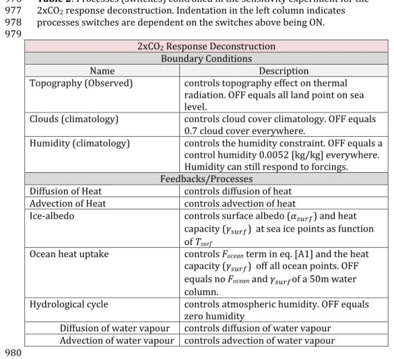
For the 2xCO2 response deconstruction experiments, we define 10 boundary 258

conditions or processes (switches; see Fig. 2). The Ice-albedo, advection and 259

diffusion of heat and water vapour, and the hydrological cycle processes are 260

defined in the same way as for the mean climate deconstruction (section 2a). The 261

remaining boundary conditions and processes are briefly listed below (and a 262

short summary is given in Table 2).

263 264

The following boundary conditions are considered:

265 266

Topography: The topography in the GREB model affects the amount of 267

atmosphere above the surface and therefore affects the emissivity of the 268

atmosphere in the thermal radiation (eq. [A9]). Regions with high topography 269

have less CO2 concentration in the thermal radiation (eq. [A9]). When the 270

topography is turned OFF, all points of the GREB model are set to sea level height 271

and have the same amount of CO2 concentration in the thermal radiation (eq.

272

[A9]).

273 274

Clouds: The cloud cover in the GREB model affects the incoming solar radiation 275

and the emissivity of the atmosphere in the thermal radiation (eq. [A9]). In 276

particular, it influences the sensitivity of the emissivity to changes in the CO2

277

concentration. A clear sky atmosphere is more sensitive to changes in the CO2

278

concentration than a fully cloud-covered atmosphere. When the cloud cover 279

switch is OFF, the observed cloud cover climatology boundary conditions are 280

replaced with a constant global mean cloud cover of 0.7. It is not set to zero to 281

avoid an impact on the global climate sensitivity, and to focus on the regional 282

effects of inhomogeneous cloud cover.

283 284

Humidity: Similarly, to the cloud cover, the amount of atmospheric water 285

vapour affects the emissivity of the atmosphere in the thermal radiation and, in 286

particular, the sensitivity to changes in the CO2 concentration (eq. [A9]). A humid 287

atmosphere is less sensitive to changes in the CO2 concentration than a dry 288

atmosphere. When the humidity switch is OFF, the constraint to the observed 289

humidity climatology (flux correction in eq. [A4]) is replaced with a constant 290

global mean humidity of 0.0052 [kg/kg]. It is again not set to zero to avoid an 291

impact on the global climate sensitivity, but to focus on the regional effects of 292

inhomogeneous humidity.

293 294

The additional feedbacks and processes considered are:

295 296

Ocean heat uptake: The ocean heat uptake in GREB is done in two ocean layers.

297

The largest part of the ocean heat is in the subsurface layer, Tocean (eq. [A3]).

298

When the ocean switch is OFF the Focean term in eq. [A1] is set to zero, equation 299

[A3] is set to zero and the heat capacity (𝛾_"#$%) off all ocean points in eq. [A1] is 300

set to that of a 50m water column.

301 302

The total number of experiments with these process switches is 640. For each 303

experiment, the GREB model is run for 50 years, starting from the original GREB 304

model climatology and the changes relative to the original GREB model 305

climatology of this experiment is presented in the MSCM database.

306

c. Scenario experiments 307

A number of different scenarios of external boundary condition changes exist in 308

the MSCM experiment database. They include different changes in the CO2

309

concentration and in the incoming solar radiation. A complete overview is given 310

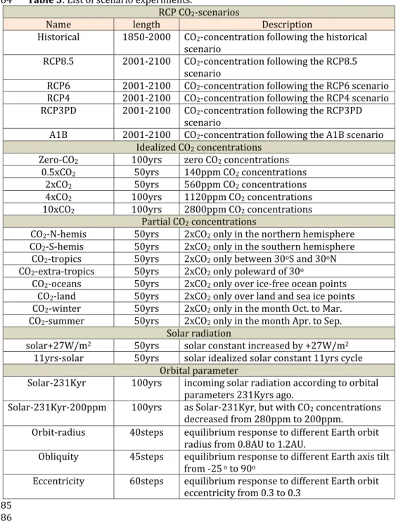
in Table 3. A short description follows below.

311

312 RCP-scenarios 313

In the Representative Concentration Pathways (RCP) scenarios the GREB model 314 is forced with time varying CO2 concentrations. All five different simulations have 315

the same historical time evolution of CO2 concentrations starting from 1850 to 316

2000, and from 2001 follow the RCP8.5, RCP6, RCP4.5, RCP2.6 and the A1B CO2

317

concentration pathways until 2100 [van Vuuren et al. 2011].

318 319

IdealizedCO2 scenarios 320

The 15 idealized CO2 concentration scenarios in the MSCM experiment database 321

focus on the non-linear time delay and regional differences in the climate 322

response to different CO2 concentrations. These were implemented in five 323

simulations in which the control CO2 concentration (340ppm) was changed in 324

the first time step to a scaled CO2 concentration of 0, 0.5, 2, 4, and 10 times the 325

control level. The 0.5xCO2 and 2xCO2 simulations are 50yrs long and the others 326

are 100yrs long.

327

Two different simulations with idealized time evolutions of CO2 concentrations 328

are conducted to study the time delay of the climate response. In one simulation, 329

the CO2 concentration is doubled in the first time step, held at this level for 30yrs 330

then returned to control levels instantaneously. In the second simulation, the CO2

331

concentration is varied between the control and 2xCO2 concentrations following 332

a sine function with a period of 30yrs, starting at the minimum of the sine 333

function at the control CO2 concentration. Both simulations are 100yrs long.

334

The third set of idealized CO2 concentration scenarios double the CO2

335

concentrations restricted to different regions or seasons. The eight regions and 336

seasons include: the Northern or Southern Hemisphere, tropics (30^oS-30^oN) or 337

extra-tropics (poleward of 30^o), land or oceans and in the month October to 338

March or in the month April to September. Each experiment is 50yrs long.

339

340 Solar radiation 341

Two different experiments with changes in the solar constant were created. In 342

the first experiment, the solar constant is increased by about 2% (+27W/m²), 343

which leads to about the same global warming as a doubling of the CO2

344

concentration [Hansen et al. 1997]. In the second experiment, the solar constant 345

oscillates at an amplitude of 1W/m² and a period of 11yrs, representing an 346

idealized variation of the incoming solar short wave radiation due to the natural 347

11yr solar cycle [Willson and Hudson 1991]. Both experiments are 50yrs long.

348 349

Idealized orbital parameters 350

A series of five simulations are done in the context of orbital forcings and the 351

related ice age cycles. In one simulation, the incoming solar radiation as function 352

of latitude and day of the year was changed to its values as it was 231Kyrs ago 353

[Berger and Loutre 1991 and Huybers 2006]. In an additional simulation, the CO2

354

concentration is reduced from 340ppm to 200ppm as observed during the peak 355

of ice age phases in combination with the incoming solar radiation changes. Both 356

simulations are 100yrs long.

357

In three sensitivity experiments, we changed the incoming solar radiation 358

according to some idealized orbital parameter changes to study the effect of the 359

most important orbital parameters. The orbital parameters changed are: the 360

distance to the sun, the Earth axis tilt relative to the Earth-Sun plane (obliquity) 361 and the eccentricity of the Earth orbit around the sun. The orbit radius was 362

changed from 0.8AU to 1.2AU in steps of 0.01AU, the obliquity from -25° to 90° in 363

steps of 2.5° and the eccentricity from 0.3 (Earth closest to the sun in July) to 0.3 364

(Earth furthest from the sun in July) in steps of 0.01. Each sensitivity experiment 365

was started from the control GREB model (1AU radius, 23.5^o obliquity and 0.017 366

eccentricity) and run for 50yrs. The last year of each simulation is presented as 367

the estimate for the equilibrium climate.

368

3. Some results of the model simulations

369

The MSCM experiment database includes a large set of experiments that address 370

many different aspects of the climate. At the same time, the GREB model has 371

limited complexity and not all aspects of the climate system are simulated in the 372

GREB experiments. The following analysis will give a short overview of some of 373

the results that can be taken from the MSCM experiments. In this we will focus 374

on aspects of general interest and on comparing the outcome to results of other 375

published studies to illustrate the strength and limitations of the GREB model in 376

this context. The discussion, however, will be incomplete, as there are simply too 377

many aspects that could be discussed in this set of experiments. We will 378

therefore focus on a general introduction and leave space for future studies to 379

address other aspects.

380

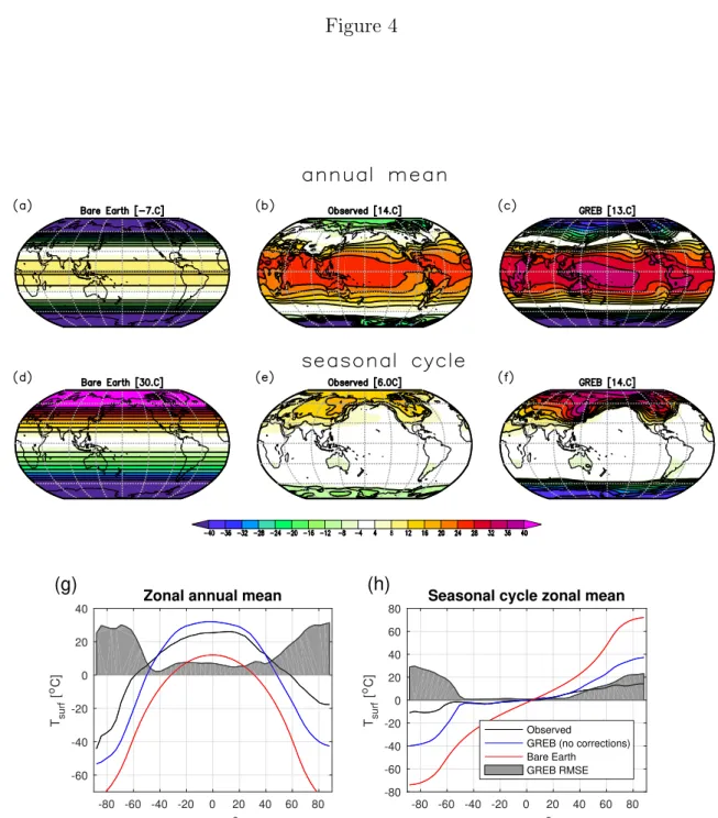
a. GREB model performance 381

The skill of the GREB model is illustrated in Figure 4, by running the GREB model 382 without the correction terms. For reference, we compare this GREB run with the 383

observed mean climate and seasonal cycle (this is identical to running the GREB 384

model with correction terms) and with a bare world. The latter is the GREB 385

model with all switches OFF (radiative balance without an atmosphere and a 386

dark surface). In comparison with the full GREB model, this illustrates how much 387

all the climate processes affect the climate.

388

The GREB model without correction terms does capture the main features of the 389

zonal mean climate, the seasonal cycle, the land-sea contrast and even smaller 390

scale structures within continents or ocean basins (e.g. seasonal cycle structure 391

within Asia or zonal temperature gradients within ocean basins). For most of the 392

globe (<50^° from the equator), the GREB model root-mean-squared error (RMSE) 393

for the annual mean Tsurf is less than 10°C relative to the observed (see Fig. 4g).

394

This is larger than for state-of-the-art CMIP-type climate models, which typically 395

have an RMSE of about 2°C [Dommenget 2012]. In particular, the regions near 396

the poles have high RMSE. It seems likely that the meridional heat transport is 397

the main limitation in the GREB model, given the too warm tropical regions and 398

the, in general, too cold polar regions and the too strong seasonal cycle in the 399

polar regions in the GREB model without correction terms.

400

The GREB model performance can be put in perspective by illustrating how 401

much the climate processes simulated in the GREB model contribute to the mean 402

climate relative to the bare world simulation (see Fig. 4). The GREB RMSE to 403

observed is about 20-30% of the RMSE of the bare world simulation (not 404

shown), suggesting that the GREB model has a relative error of about 20-30% in 405

the processes that it simulates or due to processes that it does not simulate (e.g.

406

ocean heat transport).

407

b. Mean climate deconstruction 408

Understanding what is causing the mean observed climate with its regional and 409

seasonal difference is often central for understanding climate variability and 410

change. For instance, the seasonal cycle is often considered as a first guess 411

estimate for climate sensitivity [Knutti et al. 2006]. In the following analysis, we 412

will give a short overview on how the 10 processes of the MSCM experiments 413

contribute to the mean climate and its seasonal cycle.

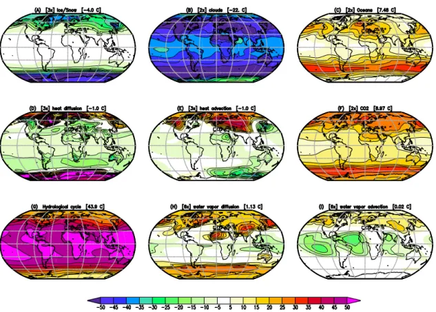
414 In Figures 5 and 6 the contribution of each of the 10 processes (except the 415

atmosphere) to the annual mean climate (Fig. 5) and its seasonal cycle (Fig. 6) 416

are shown. In each experiment, all processes are active, but the process of 417

interest and the model correction terms are turned OFF. The results are 418

compared against the complete GREB model without the model correction terms 419

(all processes active; expect model correction terms). For the hydrological we 420

will discuss some additional experiments in which the ice-albedo feedback is 421

turned OFF as well.

422

The Ice/Snow cover (Fig. 5a) has a strong cooling effect mostly at the high 423

latitudes in the cold season, which is due to the ice-albedo feedback. However, in 424

the warm season (not shown) the insulation effect of the sea ice actually leads to 425

warming, as the ocean cannot cool down as much during winter as it does 426

without sea ice.

427

Clouds (Fig. 5b) have a large net cooling effect globally due to the solar radiation 428

reflection effect dominating over the thermal radiation warming effect. It is also 429

interesting to note that the strongest cooling effect of cloud cover is over regions 430

with fairly little cloud cover (e.g. deserts and mountain regions). This is due to 431

the interaction with other climate feedbacks such as the water vapour feedback.

432

Previous studies on the cloud cover effect on the overall climate mostly focus on 433

the radiative forcings estimates, but to our best knowledge do not present the 434 overall change in surface temperature [e.g. Rossow and Zhang 1995].

435

The large ocean heat capacity slows down the seasonal cycle (Fig. 6c).

436

Subsequently, the seasons are more moderate than they would be without the 437

ocean transferring heat from warm to cold seasons. This is, in particular, 438

important in the mid and higher latitudes. The effect of the ocean heat capacity, 439

however, has also an annual mean warming effect (Fig. 5c). This is due to the 440

non-linear thermal radiation cooling. The non-linear black body negative 441

radiation feedback is stronger for warmer temperatures, which are not reached 442

in a moderated seasonal cycle with the larger ocean heat capacity.

443

The diffusion of heat reduces temperature extremes (Fig. 5d). It therefore warms 444

extremely cold regions (e.g. polar regions) and cools the hottest regions (e.g.

445

warm deserts). In global averages, this is mostly cancelled out. The advection of 446

heat has strong effects where the mean winds blow across strong temperature 447

gradients. This is mostly present in the Northern Hemisphere (Fig. 5e). The most 448

prominent feature is the strong warming of the northern European and Asian 449

continents in the cold season. In global average, warming and cooling mostly 450

cancel out.

451

The CO2 concentration leads to global averages, warming of about 9 degrees (Fig.

452

5f). Even though it is the same CO2 concentration everywhere, the warming effect 453

is different at different locations. This is discussed in more detail in DF11 and in 454

section 3c.

455 The input of water vapour into the atmosphere by the hydrological cycle leads to 456

a substantial amount of warming globally (Fig. 5g). However, we need to 457

consider that the experiment with switching OFF the hydrological cycle is the 458

only experiment in which we have a significant amount of global cooling (by 459

about -44^°C). As a result, most of the earth is below freezing temperatures and 460

therefore has a much stronger ice-albedo feedback than in any other experiment.

461

This leads to a significant amplification of the response.

462

It is instructive to repeat the experiments with the ice-albedo feedback switched 463

OFF (see supplementary Fig. 1). In these experiments, all processes show a 464

reduced impact on the annual mean temperatures, but the hydrological cycle is 465

most strongly affected by it. The ice-albedo effect almost doubles the 466

hydrological cycle response, while for all other processes the effect is about a 467

10% to 40% increase. In the following discussions, we will therefore consider 468

the hydrological cycle impact with and without ice-albedo feedback. In the 469

average of both response (Fig. 5g and SFig. 1g) the hydrological cycle has a global 470

mean impact of about +34^°C with strongest amplitudes in the tropics. It is still 471

the strongest of all processes.

472

Similar to the oceans, it dampens the seasonal cycle (Fig. 6g), but with a much 473

weaker amplitude. The transport of water vapour away from warm and moist 474

regions (e.g. tropical oceans) to cold and dry regions (e.g. high latitudes and 475

continents) leads to additional warming in the regions that gain water vapour 476

and cooling to those that lose water vapour (Fig. 6h). The effect is similar in both 477

hemispheres. The transport of water vapour along the mean wind directions has 478

stronger effects on the Northern Hemisphere than on the Southern Hemisphere, 479

since the northern hemispheric mean winds have more of a meridional 480

component, which creates advection across water vapour gradients (Fig. 6i). This 481

effect is most pronounced in the cold seasons.

482

Most processes have a predominately zonal structure. We can therefore take a 483 closer look at the zonal mean climate and seasonal cycle of all processes to get a 484

good representation of the relative importance of each process, see Fig. 7. The 485

annual mean climate is most strongly influenced by the hydrological cycle (here 486

shown as the mean of the response with and without the ice-albedo feedback).

487

The cloud cover has an opposing cooling effect, but is weaker than the warming 488

effect of the hydrological cycle. The warming effect by the ocean’s heat capacity 489

is similar in scale to that of the CO2 concentration.

490

The seasonal cycle is damped most strongly by the ocean’s heat capacity and by 491

the hydrological cycle. The later may seem unexpected, but is due to the effect 492

that the increased water vapour has a stronger warming effect in the cold 493

seasons, similarly to the greenhouse effect of CO2 concentrations. In turn, the 494

ice/snow cover and cloud cover lead to an intensification of the seasonal cycle at 495

higher latitudes. Again, the later may seem unexpected, but is due to the 496

interaction with other climate feedbacks such as the water vapour feedback, 497

which also makes the climate more strongly respond to changes in cloud cover in 498

regions where there actually is very little cloud cover (e.g. deserts).

499

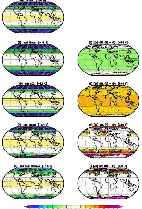
As an alternative way of understanding the role of the different process we can 500

build up the complete climate by introducing one process after the other, see 501

Figs. 8 and 9. We start with the bare earth (e.g. like our Moon) and then 502

introduce one process after the other. The order in which the processes are 503

introduced is mostly motivated by giving a good representation for each of the 504 10 processes. However, it can also be interpreted as a build up the Earth climate 505

in a somewhat historical way: We assume that initially the earth was a bare 506

planet and then the atmosphere, ocean, and all the other aspects were build up 507

over time.

508

The Bare Earth (all switches OFF) is a planet without atmosphere, ocean or ice. It 509

has an extremely strong seasonal cycle (Fig. 9a) and is much colder than our 510

current climate (Fig. 8a). It also has no regional structure other than meridional 511

temperature gradients. The combination of all climate processes will create most 512

of the regional and seasonal difference that make our current climate.

513

The atmospheric layer in the GREB model simulates two processes, if all other 514

processes are turned off: a turbulent sensible heat exchange with the surface and 515

thermal radiation due to residual trace gasses other than CO2, water vapour or 516

clouds. However, as mentioned in the appendix A1 the log-function 517

approximation leads to negative emissivity if all greenhouse gasses (CO2 and 518

water vapour) concentrations and cloud cover are zero. The negative emissivity 519

turns the atmospheric layer into a cooling effect, which dominates the impact of 520

the atmosphere in this experiment (Figs. 8b, c). This is a limitation of the GREB 521

model and the result of this experiment as such should be considered with 522

caution. In a more realistic experiment we can set the emissivity of the 523

atmosphere to zero or a very small value (0.01) to simulate the effect of the 524

atmosphere without CO2, water vapour and cloud cover, see SFig. 2. Both 525

experiments have very similar warming effects in polar regions. Suggesting that 526

the sensible heat exchange warms the surface. The residual thermal radiation 527

effect from the emissivity of 0.01 has only a minor impact (SFig. 2f and g).

528

The warming effect of the CO2 concentration is nearly uniform (Figs. 8d, e) and 529

without much of a seasonal cycle (Figs. 9d, e), if all other processes are turned 530

OFF. This accounts for a warming of about +9^°C.

531

The oceans slow down the seasonal cycle by their large heat capacity (Figs. 9f, g).

532 The effective heat capacity of the oceans is proportional to the observed mixed 533

layer in the GREB model, which causes some small variations (differences from 534

the zonal means) as seen in the seasonal cycle of the oceans. Land points are not 535

affected, since no atmospheric transport exist (advection and diffusion turned 536

OFF). The different heat capacity between oceans and land already make a 537

significant element of the regional and seasonal climate differences (Figs. 8f, g).

538

Introducing turbulent diffusion of heat in the atmosphere now enables 539

interaction between points, which has the strongest effects along coastlines and 540

in higher latitudes (Figs. 8h, i). It reduces the land-sea contrast and has strong 541

effects over land with warming in winter and cooling in summer (Figs. 9h, i). The 542

extreme climates of the winter polar region are most strongly affected by the 543

turbulent heat exchange with lower latitudes. The turbulent heat exchange 544

makes the regional climate difference again a bit more realistic.

545

The advection of heat is strongly dependent on the temperature gradients along 546

the mean wind field directions. It provides substantial heating during the winter 547

season for Europe, Russia, and western North America (Figs. 8j, k, 9j, k). The 548

structure (differences from the zonal mean) created by this process is mostly 549

caused by the prescribed mean wind climatology. In particular, the milder 550

climate in Europe compared to northeast Asia on the same latitudes, are created 551

by wind blowing from the ocean onto land. The same is true for the differences 552

between the west and east coasts of the northern North America. The climate 553 regional and seasonal structures are now already quite realistic, but the overall 554

climate is much too cold. The ice/snow cover further cools the climate, in 555

particular, the polar regions (Figs. 8l, m). This difference illustrates that the ice- 556

albedo feedback is primarily leading to cooling in higher latitudes and mostly in 557

the winter season.

558

Introducing the hydrological cycle brings the most important greenhouse gas 559

into the atmosphere: water vapour. This has an enormous warming effect 560

globally (Figs. 8n, o) and a moderate reduction in the strength of the seasonal 561

cycle (Figs. 9n, o). The resulting modelled climate is now much too warm, but 562

introducing the cloud cover cools the climate substantially (Figs. 8p, q) and leads 563

to a fairly realistic climate.

564

The atmospheric transport (diffusion and advection) brings water vapour from 565

relative moist regions to relatively dry regions (Figs. 8r, s). This leads to 566

enhanced warming in the dry and cold regions (e.g. Sahara Desert or polar 567

regions) by the water vapour thermal radiation (greenhouse) effect and cooling 568

in the regions where it came from (e.g. tropical oceans). The heating effect is 569

similar to the transport of heat and has also a strong seasonal cycle component.

570

c. 2xCO2 response deconstruction 571

The doubling of the CO2 concentrations leads to a distinct warming pattern with 572

polar amplification, a land-sea contrast and significant seasonal differences in 573

the warming rate. These structures in the warming pattern reflect the complex 574

interactions between feedbacks in the climate system and regional difference in 575

CO2 forcing pattern. The MSCM 2xCO2 response experiments are designed to help 576 understand the interactions causing this distinct warming pattern. DF11 577

discussed many aspects of these experiments with focus on the land-sea 578

contrast, the seasonal differences, and the polar amplification. We therefore will 579

focus here only on some aspects that have not been previously discussed in 580

DF11.

581

In the GREB model, we can turn OFF the atmospheric transport and therefore 582

study the local interaction without any lateral interactions. Figure 10 shows 583

three experiments in which the atmospheric transport and other processes (see 584

Figure caption) are inactive. The three experiments highlight the regional 585

difference in the CO2 forcing pattern and in the two main feedbacks (water 586

vapour and ice-albedo).

587

In the first experiment (Fig. 10a) without feedback processes, the local Tsurf

588

response is approximately directly proportional to the local CO2 forcing. The 589

regional differences are caused by differences in the cloud cover and 590

atmospheric humidity, since both influence the thermal radiation effect of CO2

591

[DF11, Kiehl and Ramanathan 1982 and Cess et al. 1993]. This causes, on 592

average, the land regions to see a stronger forcing than oceanic regions (see Fig.

593

10b). However, even over oceans we can see clear differences. For instance, the 594

warm pool of the western tropical Pacific sees less CO2 forcing than the eastern 595

tropical Pacific.

596

The ice-albedo feedback is strongly localized and it is strongest over the mid- 597

latitudes of the northern continents and at the sea ice edge of around Antarctica 598

(Figs. 10c and d). The water vapour feedback is far more wide-spread and 599

stronger (Figs. 10e and f). It is strongest in relatively warm and dry regions (e.g.

600

subtropical oceans), but also shows some clear localized features, such as the 601

strong Arabian or Mediterranean Seas warming.

602

d. Scenarios 603

The set of scenario experiments in the MSCM simulations allows us to study the 604

response of the climate system to changes in the external boundary conditions in 605

a number of different ways. In the following, we will briefly illustrate some 606

results from these scenarios and organize the discussion by the different themes 607

in scenario experiments.

608 The CMIP project has defined a number of standard CO2 concentration projection 609

simulations, that give different RCP scenarios for the future climate change, see 610

Fig. 11a. The GREB model sensitivity in these scenarios is similar to those of the 611

CMIP database [Forster et al. 2013].

612

Idealized CO2 concentration scenarios help to understand the response to the CO2

613

forcing. In Figure 11b, we show the global mean Tsurf response to different scaling 614

factors of CO2 concentrations. To first order, we can see that the global mean Tsurf

615

response follows a logarithmic CO2 concentration (e.g. any doubling of the CO2

616

concentration leads to the same global mean Tsurf response; compare 2xCO2 with 617

4xCO2 or with in Fig.11b) as suggested in other studies [Myhre et al. 1998].

618

However, this relationship does breakdown if we go to very low CO2

619

concentrations (e.g. zero CO2 concentration) illustrating that the log-function 620

approximation of the CO2 forcing effect is only valid within a narrow range far 621

away from zero CO2 concentration.

622

The transient response time to CO2 forcing can be estimated from idealized CO2

623

concentration changes, see Fig. 11c. The step-wise change in CO2 concentration 624

illustrates the response time of the global climate. In the GREB model, it takes 625

about 10yrs to get 80% of the response to a CO2 concentration change (see step- 626

function response, Fig. 11c). In turn, the response to a CO2 concentration wave 627 time evolution is a lag of about 3yrs. The fast versus slow response also leads to 628

different warming patterns with strong land-sea contrasts (not shown), that are 629

largely similar to those found in previous studies [Held et al. 2010].

630

The regional aspects of the response to a CO2 concentration can also be studied 631

by partially increasing the CO2 concentration in different regions, see Fig. 12. The 632

warming response mostly follows the regions where we partially changed the 633

CO2 concentration, but there are some interesting variations in this. The partial 634

increase in the CO2 concentration over oceans has a stronger warming impact 635

than the partial increase in the CO2 concentration over land for most Southern 636

Hemisphere land regions. In turn, the land forcing has little impact for the ocean 637

regions. The boreal winter forcing has stronger impact on the Southern 638

Hemisphere than boreal summer forcing, suggesting that the warm season 639

forcing is, in general, more important than the cold season forcing. The only 640

exception to this is the Tibet-plateau region.

641

A series of scenarios focus on the impact of solar forcing. In Figure 11d, we show 642

the response to an idealized 11yr solar cycle. The global mean Tsurf response is 643

two orders of magnitude smaller than the response to a doubling of the CO2

644

concentration, reflecting the weak amplitude of this forcing. This result is largely 645

consistent with the response found in GCM simulations [Cubasch et al. 1997], but 646

does not consider possible more complicated amplification mechanisms [Meehl 647

et al. 2009]. A change in the solar constant of +27W/m² has a global Tsurf

648 warming response similar to a doubling of the CO2 concentration, but with a 649

slightly different warming pattern, see Fig. 13. The warming pattern of a solar 650

constant change has a stronger warming where incoming sun light is stronger 651

(e.g. tropics or summer season) and a weaker warming in region with less 652

incoming sun light (e.g. higher latitudes or winter season). This is in general 653

agreement with other modelling studies [Hansen et al. 1997].

654

On longer paleo time scales (>10,000yrs), changes in the orbital parameters 655

affect the incoming sun light. Figure 14 illustrates the response to a number of 656

orbital solar radiation changes. Incoming radiation (sunlight) typical of the ice 657

age (231kyrs ago) has less incoming sunlight in the Northern Hemispheric 658

summer. However, it has every little annual global mean changes (Fig. 14a) due 659

to increases in sunlight over other regions and seasons. The Tsurf response 660

pattern in the zonal mean at the different seasons is very similar to the solar 661

forcing, but the response is slightly more zonal and seasonal differences are less 662

dominant (Fig. 14b). The response is also amplified at higher latitudes. However, 663

in the global mean there is no significant global cooling as observed during ice 664

ages. If the solar forcing is combined with a reduction in the CO2 concentration 665

(from 340ppm to 200ppm), we find a global mean cooling of -1.7^oC (Fig. 14c), 666

which is still much weaker than observed during ice ages, but is largely 667

consistent with previous studies of simulations of ice age conditions [Weaver et 668

al. 1998, Braconnot et al. 2007]. This is not unexpected since the GREB model 669

does not include an ice sheet model and, therefore, does not include glacier 670

growth feedbacks that would amplify ice age cycles.

671

A better understanding of the orbital solar radiation forcing can be gained by 672

analysing the response to idealized orbital parameter changes. We therefore 673

vary the Earth distance to the sun (radius), the earth axis tilt to the earth orbit 674

plane (obliquity) and shape of the earth orbit around the sun (eccentricity) over 675

a wider range, see Figs. 14 d-f. When the radius is changed by 10%, the Earth 676 climate becomes essentially uninhabitable, with either global mean temperature 677

above 30^oC (approx. summer mean temperature of the Sahara) or a completely 678

ice-covered snowball Earth. This suggests that the habitable zone of the Earth 679

radius is fairly small due to the positive feedbacks within the climate system 680

simulated in the GREB model (not considering long-term or more complex 681

atmospheric chemistry feedbacks) and largely consistent with previous studies 682

[Kasting et al. 1993].

683

When the obliquity is zero, the tropics become warmer and the polar regions 684

cool down further than today’s climate, as they now receive very little sunlight 685

throughout the whole year. In the extreme case, when the obliquity is 90^°, the 686

tropics become ice covered and cooler than the polar regions, which are now 687

warmer than the tropics today and ice free. The polar regions now have an 688

extreme seasonal cycle (not shown), with sunlight all day during summer and no 689

sunlight during winter. Any eccentricity increase in amplitude would lead to a 690

warmer overall climate. Thus, a perfect circle orbit around the sun has, on 691

average, the coldest climate and all of the more extreme eccentricity (elliptic) 692

orbits have warmer climates. This suggests that the warming effect of the section 693

of the orbit that has a closer transit around the sun in an eccentricity orbit 694

relative to the perfect circle orbit overcompensates the cooling effect of the more 695

remote transit around the sun in the other half of the orbit relative to the perfect 696

circle orbit.

697

4. Summary and discussion

698

In this study, we introduced the MSCM database (version: MSCM-DB v1.0) for 699

research analysis with more than 1,300 experiments. It is based on model 700

simulations with the GREB model for studies of the processes that contribute to 701

the mean climate, the response to doubling of the CO2 concentration, and 702

different scenarios with CO2 or solar radiation forcings. The GREB model is a 703

simple climate model that does not simulate internal weather variability, 704

circulation, or cloud cover changes. It provides a simple and fast null hypothesis 705

for the interactions in the climate system and its response to external forcings.

706

The GREB model without flux corrections simulates the mean observed climate 707

well and has an uncertainty of about 10^°C. The model has larger cold biases in 708

the polar regions indicating that the meridional heat transport is not strong 709

enough. Relative to a bare world without any climate processes the RMSE is 710

reduced to about 20-30% relative to observed. Thus, as a first guess, it can be 711

assumed that the GREB model simulations gives a 20-30% uncertainty in the 712

processes it simulates. Further, the GREB models emissivity function reaches 713

unphysical negative values when water vapour, CO2 and cloud cover is set to 714

zero. This is a limitation of the log-function parametrization, that can potentially 715

be revised if a new parameterization is developed that considers these cases.

716

However, it is beyond the scope of this study to develop such a new 717

parameterization and it is left for future studies.

718

The MSCM experiments for the conceptual deconstruction of the observed mean 719

climate provide a good understanding of the processes that control the annual 720

mean climate and its seasonal cycle. The cloud cover, atmospheric water vapour, 721

and the ocean heat capacity are the most important processes that determine the 722

regional difference in the annual mean climate and its seasonal cycle. The 723 observed seasonal cycle is strongly damped not only by the ocean heat capacity, 724

but also by the water vapour feedback. In turn, ice-albedo and cloud cover 725

amplify the seasonal cycle in higher latitudes.

726

The conceptual deconstruction of the response to a doubling of the CO2

727

concentration based on the MSCM experiments has mostly been discussed in 728

DF11, but some additional results shown here focused on the local forcing in 729

response without horizontal interaction. It has been shown here that the CO2

730

forcing has a clear land-sea contrast, supporting the land-sea contrast in the Tsurf

731

response. The water vapour feedback is wide-spread and most dominant over 732

the subtropical oceans, whereas the ice-albedo feedback is more localized over 733

Northern Hemispheric continents and around the sea ice border.

734

The series of scenario simulations with CO2 and solar forcing provide many 735

useful experiments to understand different aspects of the climate response. The 736

RCP and idealized CO2 forcing scenarios give good insights into the climate 737

sensitivity, regional differences, transient effects, and the role of CO2 forcing at 738

different seasons or locations. The solar forcing experiments illustrate the subtle 739

differences in the warming pattern to a CO2 forcing and the orbital solar forcing 740

illustrated elements of the climate response to long term, paleo, climate forcings.

741

In summary, the MSCM provides a wide range of experiments for understanding 742

the climate system and its response to external forcings. It builds a basis on 743

which conceptual ideas can be tested to a first-order and it provides a null 744 hypothesis for understanding complex climate interactions. Some of the 745

experiments presented here are similar to previously published simulations. In 746

general, the GREB model results agree well with the results of more complex 747

GCM simulations. It is beyond the scope of this study to discuss all aspects of the 748

experiments and their results. This will be left to future studies.

749

Future development of this MSCM database will continue and it is expected that 750

this database will grow. The development will go in several directions: the GREB 751

model performance in the processes that it currently simulates will be further 752

improved. In particular, the simulation of the hydrological cycle needs to be 753

improved to allow the use of the GREB model to study changes in precipitation.

754

Simulations of aspects of the large-scale atmospheric circulation, aerosols, 755

carbon cycle, or glaciers would further enhance the GREB model and would 756

provide a wider range of experiments to run for the MSCM database.

757

5. Code availability

758

The MSCM model code, including all required input files, to do all experiments 759

described on the MSCM homepage and in this paper, can be downloaded as 760

compressed tar archive from the MSCM homepage under 761 762

http://mscm.dkrz.de/download/mscm-web-code.tar.gz 763

764

or from the bitbucket repository under 765

766

https://bitbucket.org/tobiasbayr/mscm-web-code 767

768

The data for all the experiments of the MSCM can be accessed via the MSCM 769

webpage interface (DOI: 10.4225/03/5a8cadac8db60). The mean 770

deconstruction experiments file names have an 11 digits binary code that 771

describe the 11 process switches combination: 1=ON and 0=OFF. The digit from 772

left to right present the following processes:

773 774

1. Model corrections 775

2. Ice albedo 776

3. Cloud cover 777

4. Advection of water vapour 778

5. Diffusion of water vapour 779

6. Hydrologic cycle 780

7. Ocean 781

8. CO2

782

9. Advection of heat 783

10. Diffusion of heat 784

11. Atmosphere 785

786

For example, the data file greb.mean.decon.exp-10111111111.gad is the 787

experiment with all processes ON, but ice albedo is OFF. The 2x CO2 response 788

deconstruction experiments file names have a 10 digits binary code that describe 789

the 10 process switches combination. The digit from left to right present the 790

following processes:

791 792

1. Ocean heat uptake 793

2. Advection of water vapour 794

3. Diffusion of water vapour 795

4. Hydrologic cycle 796

5. ice albedo 797

6. Advection of heat 798

7. Diffusion of heat 799

8. Humidity (climatology) 800 9. Clouds (climatology) 801

10. Topography (Observed) 802

803

For example, the data file response.exp-0111111111.2xCO2.gad is the experiment 804

with all processes ON, but ocean heat uptake is OFF. The individual experiments 805

can be chosen from the webpage interface by selecting the desired switch 806

combinations. Alternatively, all experiments can be downloaded in a combined 807

tar-file from the webpage interface.

808 809

Acknowledgments

810

This study was supported by the ARC Centre of Excellence for Climate System 811

Science, Australian Research Council (grant CE110001028).

812