Testing model assumptions in functional regression models

SFB 823

Testing model assumptions in Testing model assumptions in Testing model assumptions in Testing model assumptions in functional regression models functional regression models functional regression models functional regression models

D is c u s s io n P a p e r

Axel Bücher, Holger Dette, Gabi Wieczorek

Nr. 27/2009

Testing model assumptions in functional regression models

Axel B¨ ucher, Holger Dette, Gabi Wieczorek Ruhr-Universit¨ at Bochum

Fakult¨ at f¨ ur Mathematik 44780 Bochum, Germany

e-mail: axel.buecher@ruhr-uni-bochum.de e-mail: holger.dette@ruhr-uni-bochum.de

September 28, 2009

Abstract

In the functional regression model where the responses are curves new tests for the func- tional form of the regression and the variance function are proposed, which are based on a stochastic process estimatingL²-distances. Our approach avoids the explicit estimation of the functional regression and it is shown that normalized versions of the proposed test statistics converge weakly. The finite sample properties of the tests are illustrated by means of a small simulation study. It is also demonstrated that for small samples bootstrap versions of the tests improve the quality of the approximation of the nominal level.

Keywords and Phrases: goodness-of-fit tests, functional data, parametric bootstrap, tests for het- eroscedasticity

AMS Subject Classification: 62G10

1 Introduction

Since the pioneering work by Ramsay and Dalzell (1991) on regression analysis for functional data this topic has received considerable attention in the recent literature. The interest in statistical techniques enabling to take into account the functional nature of data stems from the fact that nowadays in many applications (for instance in climatology, remote sensing, linguistics, . . .) the data comes from the observation of a continuous phenomenon over time. For a review on the statistical problems and techniques for functional data we refer to the monographs of Ramsay and Silverman (2005) and Ferraty and Vieu (2006). In these models either predictors or responses can be viewed as random functions. The data typically appears when the value of a variable is repeatedly recorded on a dense grid of time points for a sample of subjects. While many authors consider the problem of estimating the regression or generalizing classical concepts of multivariate statistics as principal component or discrimination analysis to the situation where the data are curves [see for example Besse and Ramsay (1986), Faraway (1997), Kneip and Utikal (2001), Cuevas

et al. (2002), Ferraty and Vieu (2003), Escabias et al. (2004) or M¨uller and Stadtm¨uller (2005) among many others others], much less attention has been paid to the problem of testing model assumptions when analyzing functional data.

Many authors discussed the problem of testing hypotheses in a linear functional data model. For example, Cardot et al. (2003), M¨uller and Stadtm¨uller (2005) and Cardot et al. (2004) considered the problem of testing a simple hypothesis in the case where the response is real and the predictor is a random function, while Mas (2007) investigated a test for the mean of random curves. Recently Shen and Faraway (2004) and Yang et al. (2007) discussed anF-test in a linear longitudinal data model, while Kokoszka et al. (2008) tested for lack of dependence in a functional linear model where both response and predictor are curves.

The present work considers the problem of testing model assumptions in the nonparametric func- tional regression model

Y_i(u) = m(u, t_i) +ε(u, t_i), t_i ∈[0,1], i= 1, . . . , n, (1.1) where u varies (without loss of generality) in the interval [0,1]. Our main concern deals with the problem of validating a parametric assumption of the form

Y_i(u) = g(u, t_i, β) +ε(u, t_i) , t_i ∈[0,1], i= 1, . . . , n, (1.2) where g is a given parametric functional regression model and β : [0,1]→R^k denotes a function, which depends either on the variable u or on t (note that both cases correspond to a different parametric modeling of the functional data). The latter model has been considered in the linear context by numerous authors. In particular Shen and Faraway (2004) and Yang et al. (2007) have proposed generalizations of the F-test for modelY(u) =x^Tβ(u) +ε(u) and used these methods to analyze some data from Ergonomics. While in this work the predictor x is considered as discrete (as in the classical ANOVA model) we concentrate in the present paper on the case where the variable t in (1.2) varies in continuous way. Our work is inspired by the recent paper of Hlubinka and Prchal (2007), who proposed a functional regression model of the form (1.2) to study the time-variation of vertical atmospheric radiation profiles by means of functional regression models.

These authors assumed that the parameter (function)β depends on the value t.

In Section 2 we introduce some notation and propose a test for the hypothesis that the regression function in the nonparametric functional regression model (1.1) is of a specific parametric form as given in (1.2) with a function β depending on the variableu, that is

H₀ :m(u, t) = g(u, t, β(u)) (1.3)

for some parametric function g and a parameter β : [0,1] → R^k. The case, where the parameter depends on t is investigated in Section 3, where we consider the hypothesis

H₀ :m(u, t) =h(u, t, γ(t)) (1.4)

for a parametric function h and some functionγ : [0,1]→R^k. Finally, we discuss in Section 4 the problem of testing parametric assumptions regarding the second order properties of the process Y(u). More precisely, if r(t, u, v) = Cov(ε(u, t), ε(v, t)) denotes the covariance of the observations Y(u) and Y(v), we are interested in the hypothesis

H₀ :r(t, u, v) = r(u, v), (1.5)

which corresponds to the case of homoscedasticity. Note that this assumption is necessary for the application of theF-tests proposed by Shen and Faraway (2004) and Yang et al. (2007). Moreover, this assumption was also made by Hlubinka and Prchal (2007) who proposed a nonlinear functional regression model for the analysis of changes in atmospheric radiation. The proposed tests for the hypotheses (1.3), (1.4) and (1.5) are very simple and are based on stochastic processes of empirical L²-distances between the nonparametric and parametric functional regression model. We prove weak convergence of these processes under the null hypothesis and fixed alternatives and, as a consequence, asymptotic normality of functionals of these processes. In Section 5 we demonstrate by means of a simulation study that for moderate sample sizes the quantiles of the asymptotic distribution provide a rather accurate approximation of the nominal level. On the other hand - for small sample sizes - a wild bootstrap version of the test is proposed and its accuracy is also investigated. Finally, some technical details are given in an Appendix.

2 A process of empirical L

-distances for testing (1.3)

Consider the nonparametric functional regression model defined by (1.1) and assume that n inde- pendent observations are available at distinctive points 0 ≤t₁ <· · · < t_n ≤1. For the discussion of the asymptotic properties of the tests proposed in this paper we will assume that the design points t₁, . . . , t_n satisfy

maxn i=2

Z ti

ti−1

h(t)dt− 1 n

=o(n^−(1+γ)), (2.1)

whereh∈Lip_γ[0,1] is a strictly positive (unknown) density on the interval [0,1], which is Lipschitz continuous of order γ >1/2 [see Sacks and Ylvisacker (1970)].

For the construction of a test for the hypothesis (1.3) of a parametric functional regression model we consider the class of parametric models

M={g(·,·, β(·)) : [0,1]×[0,1]−→R|β : [0,1]−→Θ},

where Θ is some subset of R^k. For the sake of transparency we first discuss the case of testing the hypothesis of a linear functional regression model, that is

H₀ :m(u, t) =g(u, t, β(u)) =β(u)^Tf(u, t) , (2.2) wheref(u, t) = (f₁(u, t), . . . , f_k(u, t))^T are given regression functions. We define for fixedu∈[0,1]

the inner product

hp, qi_u = Z

p(u, t)q(u, t)h(t)dt.

on the space of functions defined on the unit square on [0,1]² with corresponding norm|| · ||_u, and consider

M_u² = inf

β(u)||m(u,·)−β(u)^Tf(u,·)||²_u

as the minimal distance from m to functions of the form (2.2). A standard result from Hilbert space theory [see Achieser (1956)] yields that M_u² can be expressed as a ratio of two Gramian determinants, i.e.

M_u² = Γ_u(m, f₁, . . . , f_k) Γ_u(f₁, . . . f_k) ,

where Γ_u(p₁, . . . p_k) = det(hp_i, p_ji_u)i,j=1,...,k is the Gramian determinant of the function p₁, . . . , p_k. In order to obtain an estimator for M_u² we replace the inner products A_u,0 = hm, mi_u, A_u,p = hm, fpiu and Bu,p,q =hfp, fqiu by their empirical counterparts

Aˆ_u,0 = 1 n−1

n

X

i=2

Y_i(u)Yi−1(u), Aˆ_u,p = 1

n

n

X

i=1

Y_i(u)f_p(u, t_i), Bˆ_u,p,q = 1

n

n

X

i=1

f_p(u, t_i)f_q(u, t_i), where p, q = 1, . . . , k. This yields a canonical estimate

Mˆ_u² =

Aˆu,0 Aˆu,1 · · · Aˆu,k

Aˆ_u,1 Bˆ_u,1,1 · · · Bˆ_u,1,k ... ... . .. ... Aˆu,k Bˆu,k,1 · · · Bˆu,k,k

Bˆ_u,1,1 · · · Bˆ_u,1,k ... . .. ... Bˆ_u,k,1 · · · Bˆ_u,k,k

(2.3)

of the L²-distance M_u². In the following discussion we will study the asymptotic properties of the process {Mˆ_u²}_u∈[0,1]. Denote by

Lip^unif_γ [0,1] = {f =f(x,·) :|f(x, t)−f(x, s)| ≤C|s−t|^γ;s, t ∈[0,1]} (2.4) the set of all functions f : [0,1]×[0,1] → R satisfying a uniform Lipschitz condition (in other words, the constant C in (2.4) does not depend on x) and assume that for some γ > 1/2 and for all (t, u, v)∈[0,1]³

f_j(u,·), f_j(·, t)∈Lip^unif_γ [0,1] j = 1, . . . , k m(u,·), m(·, t)∈Lip^unif_γ [0,1],

r(·, u, v), r(t,·, v), r(t, u,·)∈Lip^unif_γ [0,1], where

r(t, u, v) = E[ε(u, t)ε(v, t)]

denotes the covariance of the (centered) errors at the point t. The following result specifies the asymptotic properties of the stochastic process{Tˆ_u−M_u²}u∈[0,1]. Throughout this paper the symbol

=⇒ denotes weak convergence.

Theorem 2.1. If the assumptions stated in this section are satisfied and the linear hypothesis (2.2) has to be tested we have as n→ ∞

√n( ˆT_u²−M_u²) =⇒G,

in C[0,1], where G is a centered Gaussian process with covariance k=k(u, v) given by k(u, v) =

Z

r²(t, u, v)h(t)dt (2.5)

+ 4 Z

r(t, u, v)(m(u, t)−g(u, t, β₀(u)))(m(v, t)−g(v, t, β₀(v)))h(t)dt and

β₀(u) = argmin_β||m(u,·)−g(v,·, β)||²_u (2.6) corresponds to the parameter of the best approximation of the function m(u,·) by the parametric regression model.

Proof of Theorem 2.1. We assume without loss of generality that the functionsf₁(u,·), . . . , f_k(u,·) are orthonormal with respect to the inner producthp, qi_u. Then the minimalL²-distance obtained by the best approximation simplifies to

M_u² =A_u,0−

k

X

p=1

A²_u,p It is easy to see that the statistics ˆA_u,p and ˆB_u,p,q are √

n consistent estimates of the quantities hm, fpiu = 0 and hfp, fqi=δp,q, respectively, and consequently we obtain for the statistic in (2.3)

T_n(u) =√ n

( Aˆ_u,0−

k

X

p=1

Aˆ²_u,p−M_u² )

+o_p(1) = ¯T_n(u) +o_P(1)

uniformly with respect tou∈[0,1], where the last equality defines the process ¯T_n(u) in an obvious manner. For the proof of weak convergence we have to show

( ¯T_n(u₁), . . . ,T¯_n(u_m))−→^D (G(u₁), . . . , G(u_m)) ∀u₁, . . . , u_m ∈[0,1], m∈N Tightness of the sequence ( ¯Tn)n∈N.

The convergence of the finite dimensional distributions follows from Theorem 2.1 and its proof in Dette et al. (1999). For a proof of tightness we use the decomposition ¯T_n(u) = U_n(u) +V_n(u) with

U_n(u) = √

n Aˆ_u,0−EAˆ_u,0−(

k

X

p=1

Aˆ²_u,p−EAˆ²_u,p)

V_n(u) = √

n EAˆ_u,0− hm, mi_u−(

k

X

p=1

EAˆ²_u,p− hm, f_pi_u) .

Consequently, it is sufficient to show that the (deterministic) sequence V_n(u) converges uniformly to 0, i.e.

sup

u∈[0,1]

|V_n(u)|=o(1), (2.7)

and that the process{Un(u)}u∈[0,1] is tight. For this purpose we use Theorem 12.3 from Billingsley (1968) and show that there are constants α > 0, γ ≥ 0 and a nondecreasing, continuous function F on [0,1] such that

E[|U_n(u)−U_n(v)|^γ]≤ |F(u)−F(v)|^α. (2.8) We first prove (2.7) and introduce the decomposition

V_n(u) =√

n V_n0(u)−

k

X

p=1

V_np(u)

with V_n0(u) =EAˆ_u,0− hm, mi_u and V_np(u) = EAˆ²_u,p− hm, f_pi²_u. Assertion (2.7) follows from sup

u∈[0,1]

|V_np(u)|=o(n⁻¹²) , p= 0, . . . , k (2.9) We consider exemplarily the first summand V_n0(u), which can be represented as

V_n0(u) = A₁(u) +A₂(u) +A₃(u) with

A₁(u) = 1 n−1

n

X

i=1

m²(u, t_i)− hm, mi_u A2(u) = − 1

n−1

n

X

i=2

m(u, ti)(m(u, ti)−m(u, ti−1)) A₃(u) = − 1

n−1m(u, t₁).

Using the the fact that m²(u,·) ∈ Lip^unif_γ [0,1] and taking into account that maxⁿ_i=2|t_i −ti−1| = O(n^−γ) =o(n⁻¹²), by (2.1), we obtain that all terms are of order o(n^−1/2), uniformly with respect tou∈[0,1]. This proves (2.9) forp= 0 and similar arguments for the remaining terms show that (2.7) holds.

In order to show that condition (2.8) is valid we calculate E

(U_n(u)−U_n(v))²

= n(B₁+B₂+B₃+B₄),

where

B₁ = Var( ˆA_u,0) + Var( ˆA_v,0)−2 Cov( ˆA_u,0,Aˆ_v,0), B₂ = Var(

k

X

p=1

Aˆ²_u,p) + Var(

k

X

p=1

Aˆ²_v,p)−2 Cov(

k

X

p=1

Aˆ²_u,p,

k

X

p=1

Aˆ²_v,p),

B₃ = 2 Cov( ˆA_u,0,

k

X

p=1

Aˆ²_v,p)−2 Cov( ˆA_u,0,

k

X

p=1

Aˆ²_u,p),

B₄ = 2 Cov(

k

X

p=1

Aˆ²_u,p,Aˆ_v,0)−2 Cov( ˆA_v,0,

k

X

p=1

Aˆ²_v,p).

We now show that it is possible to find, for each term B_i = B_i(u, v) (i = 1, . . . ,4) a constant C such that

n B_i(u, v)≤C|u−v|^γ,

which proves condition (2.8). For this purpose we exemplarily consider the expression B₁, the corresponding statements for the other terms follow along similar lines. A straightforward but tedious calculation yields

Cov( ˆA_u,0,Aˆ_v,0) = 1 (n−1)²

n

X

i=2

m(u, ti−1)m(v, ti−1)r(t_i, u, v) +m(u, t_i)m(v, t_i)r(ti−1, u, v) +r(t_i, u, v)r(ti−1, u, v)

+

n

X

i=3

m(u, t_i)m(v, ti−2)r(ti−1, u, v) +m(v, t_i)m(u, ti−2)r(ti−1, u, v)

, and we therefore obtain B₁ = ˜B₁(u, v) + ˜B₁(v, u) with

B˜₁(u, v) = 1 (n−1)²

n

X

i=2

m(u, ti−1)²r(t_i, u, u)−m(u, ti−1)m(v, ti−1)r(t_i, u, v) +m(u, t_i)²r(t_i−1, u, u)−m(u, t_i)m(v, t_i)r(t_i−1, u, v) +r(ti, u, u)r(ti−1, u, u)−r(ti, u, v)r(ti−1, u, v) +2

n

X

i=3

m(u, t_i)m(u, t_i−2)r(t_i−1, u, u)−m(u, t_i)m(v, t_i−2)r(t_i−1, u, v)

. A typical summand in ˜B₁ can be estimated by

|m(u, ti−1)²r(t_i, u, u)−m(u, ti−1)m(v, ti−1)r(t_i, u, v)| ≤C|u−v|^γ

using the Lipschitz property of the functions r and m. All other summands are treated similarly, and we obtain

B1 =B1(u, v)≤ 1

n−1C|u−v|^γ, which proves assertion (2.8) and completes the proof of Theorem 1.

2

Remark 2.2. The assertion of Theorem 2.2 remains also valid, if the general hypothesis (1.3) of nonlinear functional regression models has to be tested, and we will indicate the arguments for proving this assertion here briefly. First note that the estimate ˆA_u,0 can be rewritten as

Aˆ_u,0 = 1 n

n

X

i=1

Y_i²(u)−σˆ²_u+o_p( 1

√n), where

ˆ

σ_u² = 1 2(n−1)

n

X

i=2

(Y_i(u)−Yi−1(u))² denotes an estimate of the integrated variance

Z 1

0

Var (ε(u, t))h(t)dt= Z 1

0

r²(t, u, u)h(t)dt

at the pointu∈[0,1] [see for example Rice (1984)]. Now a straightforward calculation shows that the estimate ˆM_u² is essentially the sum of squared residuals, i.e.

Mˆ_u² = argmin_β 1 n

n

X

i=1

Y_i²(u)−β^Tf(u, ti)2

−σˆ_u²+op( 1

√n) (2.10)

uniformly with respect to u ∈ [0,1]. Obviously, this concept can be easily generalized to the problem of testing the hypothesis of a nonlinear functional regression model. To be precise we assume that for each u ∈ [0,1] the function g_u : t 7→ g(u, t, β_u) satisfies the standard regularity conditions of a nonlinear regression model [see for example Gallant (1987) or Seber and Wild (1989)]. In particular we assume the set Θ ⊂ R^k is a compact set with non-empty interior and that for all u, t ∈[0,1] the function

g(u, t, β) is twice continuously differentiable w.r.t. β and satisfies

g(u,·, β), g(·, t, β)∈Lip^unif_γ [0,1].

We recall the definition (2.6) of the parameter corresponding to best L²-approximation of the function m(u,·) : [0,1] → R by parametric functions of the form {g(u,·, βu) | βu ∈ Θ}, where we assume for each u ∈ [0,1] the existence of the minimum β₀(u) at a unique interior point of the compact space Θ. The L²-distance between the function m(u,·) and its best approximation g(u,·, β0(u)) in the parametric class is now defined by

M_u² = Z 1

0

(m(u, t)−g(u, t, β₀(u)))²h(t)dt.

In order to investigate whether the hypothesis (1.3) is satisfied let for each u∈[0,1]

βˆ₀(u) = arginf_β

n

X

i=1

(Y_i(u)−g(u, t_i, β))² (2.11)

denote the nonlinear least squares estimate (here and throughout this paper it is assumed that the infimum in (2.11) is attained at a unique interior point of Θ⊂R^k) and observing (2.11) we obtain as the analogue of (2.3) the statistic

Tˆ_u² = 1 n

n

X

i=1

(Y_i(u)−g(u, t_i,βˆ₀(u)))² −ˆσ_u². (2.12) It follows by similar arguments as in Brodeau (1993) that

Tˆ_u² = 1 n

n

X

i=2

εi(u, ti)εi(u, ti−1)− 2 n

n

X

i=1

(m(u, ti)−g(u, ti, β0(u))ε(u, ti) +M_u²+op( 1

√n) uniformly with respect tu u∈[0,1], and a similar reasoning as presented in the proof of Theorem

2.1 shows that √

n ( ˆT_u²−M_u²) =⇒G,

where the covariance structure of the Gaussian process G is specified in (2.5). The details are omitted for the sake of brevity.

Note that the null hypotheses (1.3) is satisfied if and only ifM_u² = 0 for allu∈[0,1]. Consequently, a consistent test can be obtained by rejecting the null hypotheses for large values of a Cram´er-von- Mises or a Kolmogoroff-Smirnov functional of the process {Tˆ_u}_u∈[0,1]. Under the null hypothesis the covariance kernel of the limiting process Gin Theorem 1 reduces to

k(u, v)^H=⁰ Z 1

0

r²(t, u, v)h(t)dt and by the continuous mapping theorem it follows that the statistic

√n Z 1

0

Tˆ_u²du

converges weakly to a centered normal distribution with variance R1 0

R1

0 k(u, v)dudv. Therefore, it remains to estimate the asymptotic variance, and we propose to use

ˆ s²_n=

Z 1

0

Z 1

0

ˆk(u, v)dudv, where the estimate of the covariance kernel k(u, v) is defined by

ˆk(u, v) = 1 4(n−3)

n−2

X

i=2

S_i(u)S_i(v)S_i+2(u)S_i+2(v). (2.13) withS_i(u) = Y_i(u)−Yi−1(u). The following result shows that under the null hypothesis the statistic ˆ

s²_n is a consistent estimate of the asymptotic variance. The technical details of the proof are given in the Appendix.

Proposition 2.2 Under the assumptions of Theorem 1 we have k(u, v) =ˆ k(u, v) +O_p(n^−1/2) uniformly with respect to u, v ∈[0,1].

Theorem 2.1 and Proposition 2.2 provide an asymptotic levelαtest by rejecting the null hypothesis (1.3) if

T_n=

√n q

R1 0

R1

0 ˆk(u, v)du dv Z 1

0

Tˆ_u²du > u1−α, (2.14)

where u1−α denotes the (1−α) quantile of the standard normal distribution. The finite sample properties of this test and a corresponding bootstrap version will be illustrated in Section 5.

3 A test for the hypothesis (1.4)

We now consider the problem of testing the hypothesis (1.4) in the functional regression model defined by (1.1) and assume that n independent observations according to the model (??) are available. For this purpose we define for fixed t∈[0,1] the L²-distance

M_t² = inf

γt

Z 1

0

(m(u, t)−h(u, t, γ_t))²du. (3.1) We only deal with the linear case, that is

h(u, t, γ(t)) =γ(t)^Tf(u, t)

for some given regression functions f(u, t) = (f₁(u, t), . . . , f_k(u, t)) and denote by γ₀(t) the func- tion, which yields to the minimal values in (3.1). As a global measure of deviance from the null hypothesis we consider the functional

M² = Z 1

0

M_t²h(t)dt, (3.2)

and obviously the hypothesis H0 :M² = 0 is equivalent to (1.4).

Similarly as in Section 2, standard Hilbert space theory shows that the distance M_t² can be ex- pressed as a ratio of two Gramian determinants

M_t² = Γ_t(m, f₁, . . . , f_k)

Γ(f₁, . . . , f_k) , (3.3)

where Γ_t(p₁, . . . , p_l) = det((hp_i, p_ji_t)^l_i,j=1) and the inner products are now calculated with respect to the variable u, that is

hf, gi_t= Z 1

0

f(u, t)g(u, t)du.

For the time ti we can “estimate” the entries of the matrix in the numerator of (3.3) by Bˆi,0 =

Z

Yi(u)Yi−1(u)du, Bˆ_i,p =

Z

Y_i(u)f_p(u, t_i)du, Cˆ_i,p =

Z

Yi−1(u)f_p(u, ti−1)du= ˆBi−1,p, and define

Mˆ_t²

i =

Bˆi,0 Bˆi,1 · · · Bˆi,k

Cˆ_i,1 hf₁, f₁i_ti · · · hf₁, f_ki_ti ... ... . .. ... Cˆ_i,k hf_k, f₁i_ti · · · hf_k, f_ki_ti

hf₁, f₁i_ti · · · hf₁, f_ki_ti ... . .. ... hfk, f1iti · · · hfk, fkiti

(3.4)

as an estimator forM_t²_i. Note that we estimate the entries in the upper first column by ˆC_i,p rather than ˆB_i,p in order to assure that the statistic ˆM_t²

i is asymptotically unbiased. However, because only one observation is made at timet_i, the variance of ˆM_t²

i is not converging to 0 with increasing sample size. As a consequence, the statistic ˆM_t²_i is not a consistent estimate for M_t²_i. Nevertheless, a consistent estimate for the measure defined in (3.2) can be obtained by averaging the quantities Mˆ_t²

i, that is

Mˆ² = 1 n−1

n

X

i=2

M_t²

i. (3.5)

Similarly, consistent estimates of M_t² at a particular point t can be obtained by local averages.

Theorem 3.1. Under the assumptions of Section 2 the estimate Mˆ² defined in (3.5) is consistent for M² =R1

0 M_t²dt. More precisely, we have as n→ ∞

√n−1( ˆM²−M²)→ N^D (0, σ²), where the asymptotic variance is given by

σ² = Z 1

0

Z

[0,1]²

r(u, v, t)−(P_u,tr)(v)

r(u, v, t)−(P_v,tr)(u) du dv + 4

Z

[0,1]²

r(u, v, t) m(u, t)−(P_tm)(u)

m(v, t)−(P_tm)(v) du dv

h(t)dt, and (P_tm)(u) = γ_t,0^T f(u, t) and (P_u,tr)(v) = γ_u,t,0^T f(v, t) denote the orthogonal projections of the function m(·, t) and r(u,·, t) on the set span{f₁(·, t), . . . , f_k(·, t)}, respectively, that is

Z 1

0

(m(u, t)−γ_t,0^T f(u, t))²du = inf

γt

Z 1

0

(m(u, t)−γ_t^Tf(u, t))²du=M_t²,

Z 1

0

(r(u, v, t)−γ_u,t,0^T f(v, t))²dv = inf

γu,t

Z 1

0

(r(u, v, t)−γ_u,t^T f(v, t))²dv.

Proof of Theorem 3.1. Without loss of generality we may assume that the functions f₁, . . . , f_k are orthonormal and therefore the minimal distance in (3.3) and its estimator defined in (3.4) simplify to

M_t²_i = hm, mi_ti−

k

X

p=1

hm, f_pi²_ti, Mˆ_t²

i = ˆB_i,0−

k

X

p=1

Bˆ_i,pCˆ_i,p,

respectively. A careful calculation of the moments of the random variables in the latter expression yields

E[ ˆB_i,0] = hm, mi_ti+O(n^−γ), E[ ˆB_i,pCˆ_i,p] = hm, f_pi²_t

i +O(n^−γ),

Var(B_i,0) = Z

r(u, v, t_i)²du dv+ 2 Z

r(u, v, t_i)m(u, t_i)m(v, t_i)du dv+ (O(n^−γ), Cov( ˆB_i,pCˆ_i,p,Bˆ_i,qCˆ_i,q) =

Z

r(u, v, t_i)f_p(u, t_i)f_q(v, t_i)du dv

2hm, f_pi_tihm, f_qi_ti +

Z

r(u, v, t_i)f_p(u, t_i)f_q(v, t_i)du dv

+O(n^−γ), Cov( ˆBi,0,Bˆi,pCˆi,p) = 2

Z

r(u, v, ti)m(u, ti)fp(v, t)du dthm, fpiti

+ Z

r(u, v, t_i)r(u, w, t_i)f_p(v, t_i)f_p(w, t_i)du dv dw+O(n^−γ), Cov( ˆB_i,0,Bˆi−1,0) = 2

Z

r(u, v, t_i)m(u, t_i)m(v, t_i)du dv, Cov( ˆB_i,0,,Bˆi−1,pCˆi−1,p) =

Z

r(u, v, t_i)m(u, t_i)f_p(v, t_i)du dvhm, f_pi_ti+O(n^−γ)

= Cov( ˆB_i−1,p,Bˆ_i,0Cˆ_i,p), Cov( ˆB_i,pCˆ_i,p,Bˆi−1,qCˆi−1,q) =

Z

r(u, v, t_i)f_p(u, t_i)f_q(v, t_i)du dvhm, f_pi_tihm, f_qi_ti+O(n^−γ).

The sequence ˆM_t²₂, . . . ,Mˆ_t²_n forms a triangular array of one-dependent random variable and as a consequence all covariances corresponding to a lag larger than one vanish. Therefore the variance of the standardized mean

σ_n² = Var( 1

√n−1

n

X

i=2

M_t²_i)

is given by σ_n² = 1

n−1

n

X

i=2

Var(B_i,0) +

k

X

p,q=1

Cov( ˆB_i,pCˆ_i,p,Bˆ_i,qCˆ_i,q)−2

k

X

p=1

Cov( ˆB_i,0,Bˆ_i,pCˆ_i,p)

+ 2 Cov( ˆB_i,0, Bi−1,0)−2

k

X

p=1

Cov( ˆB_i,0,Bˆi−1,pCˆi−1,p)

−2

k

X

p=1

Cov( ˆBi−1,0,Bˆ_i,pCˆ_i,p) + 2

k

X

p,q=1

Cov( ˆB_i,pCˆ_i,p,Bˆi−1,qCˆi−1,q)

+O(n^−γ)

= Z 1

0

Z

r(u, v, t)²du dv−2

k

X

p=1

Z

r(u, v, t)r(u, w, t)fp(v, t)fq(w, t)du dv dw

+

k

X

p,q=1

Z

r(u, v, t)f_p(u, t)f_q(v, t)du dv 2

+ 4 Z

r(u, v, t)m(u, t)m(v, t)du dv−8

p

X

i=1

Z

r(u, v, t)m(u, t)fp(v, t)du, dvhm, fpit

+ 4

k

X

p,q=1

Z

r(u, v, t)fp(u, t)fq(v, t)du dvhm, fpithm, fqit

dt+O(n^−γ)

= σ²+O(n^−γ).

Here the last equality uses the fact that under the assumption of orthonormality the orthogonal projection Ptm and Pu,tr are given by

(Ptm)(u) =

k

X

p=1

hm, fpitfp(u, t),

(P_u,tr)(v) =

k

X

p=1

hr(u,·), f_pi_tf_p(v, t).

The assertion of the theorem now follows by the classical central limit theorem for m-dependent random variables (see Orey (1958)).

2

Under the null hypothesis the variance of the limiting normal distribution simplifies to σ^{2 H}=⁰

Z 1

0

Z

[0,1]²

r(u, v, t)−(P_u,tr)(v)

r(u, v, t)−(P_v,tr)(u)

d(u, v)h(t)dt.

We propose to estimate this variance by ˆ

σ² = 1

4(n−3)

n−2

X

i=2

Z

[0,1]²

S_i(u) S_i(v)− Z 1

0

S_i(x)f(x, t_i)^T dxA⁻¹_i f(v, t_i)

×S_i+2(v) S_i+2(u)− Z 1

0

S_i+2(x)f(x, t_i+2)^T dx A⁻¹_i+2f(u, t_i+2

d(u, v), whereS_i(u) = Y_i(u)−Yi−1(u) andA_i =R1

0 f(u, t_i)f(u, t_i)^T du∈R^k×k. Observing that the orthog- onal projection (P_u,tr)(v) is given by

P_u,tr(v) =γ_u,t,0^T f(v, t) = Z 1

0

r(u, x, t)f(x, t)^T dx Z 1

0

f(x, t)(f(x, t)^T dx ⁻¹

f(v, t) it follows by a similar calculation as in the proof of Theorem 3.1 that ˆσ²is a√

n-consistent estimator for σ². Therefore we obtain an asymptotic levelα test for the hypothesis (1.4) by rejecting H₀ if

rn−1 ˆ σ²

Mˆ² > u_1−α, (3.6)

where u_1−α denotes the (1−α) quantile of the standard normal distribution.

4 Testing homoscedasticity

In this section we address the problem of testing the hypothesis (1.5) of homoscedastic errors in the functional regression model (1.1). Motivated by the discussion in Section 2 and 3 we propose the following measure of heteroscedasticity at a point (u, v)∈[0,1]²

τ²(u, v) = min

a∈R

||r(·, u, v)−a||² = Z 1

0

r²(t, u, v)h(t)dt− Z 1

0

r(t, u, v)h(t)dt ²

. (4.1) Note that τ²(u, v) = 0 a.e. if and only if the covariance function does not depend ont, that is the hypothesis (1.5) of homoscedasticity is valid. An estimator for the quantity R1

0 r²(t, u, v)h(t)dt in (4.1) has been proposed in (2.13), and for the second term we will use a similar estimate based on the statistic

k(u, v) =˜ 1 2(n−1)

n

X

i=2

S_i(u)S_i(v),

whereSi(u) =Yi(u)−Yi−1(u). We therefore obtain as an estimator of the process{τ²(u, v)}u,v∈[0,1]

ˆ

τ_n²(u, v) = 1 4(n−3)

n−2

X

i=2

S_i(u)S_i(v)S_i+1(u)S_i+2(v)− 1 2(n−1)

n

X

i=2

S_i(u)S_i(v)

!2

. The asymptotic properties of this random variable are specified in the following result.

Theorem 4.1. Assume that the third and fourth moments

d₁(t, u, v, w) = E[ε(u, t)ε(v, t)ε(w, t)]

d₂(t, u, v, w, x) = E[ε(u, t)ε(v, t)ε(w, t)ε(x, t)]

of the error process ε(u, t) exist and are elements of Lip^unif_γ [0,1] for every argument. If the as- sumptions of Section 2 are satisfied we have as n → ∞

4√

n(ˆτ_n²(u, v)−τ²(u, v)) =⇒G

in C[0,1]². Here G is a centered Gaussian field on [0,1]² whose covariance structure under the null hypothesis of homoscedasticity is given by

k((u₁, v₁),(u₂, v₂)) := Cov (G(u₁, v₁), G(u₂, v₂))

= 6D⁽²⁾₂ (u1, v1, u2, v2)−12D₂^(r,1,1)(u1, v1, u2, v2) + 8D^(r,1,1)₂ (u1, u2, v1, v2) + 8D^(r,1,1)₂ (u1, v2, v1, u2) +6J(u₁, v₁, u₂, v₂, u₁, v₁, u₂, v₂) + 4J(u₁, u₂, v₁, v₂, u₁, u₂, v₁, v₂)

+4J(u₁, v₂, v₁, u₂, u₁, v₂, v₁, u₂)−8J(u₁, v₁, u₂, v₂, u₁, u₂, v₁, v₂)

−8J(u₁, v₂, u₂, v₂, u₁, v₂, v₁, u₂) + 8J(u₁, v₁, u₂, v₂, u₁, v₂, v₁, u₂)

+2D^(r)₁ (u1, u2, v1, v2) + 2D₁^(r)(u1, v2, v1, u2) + 2D₁^(r)(v1, u2, u1, v2) + 2D^(r)₁ (v1, v2, u1, u2) where the following notations have been used

D⁽²⁾₂ (u₁, v₁, u₂, v₂) = Z 1

0

d₂(t, u₁, v₁, u₂, v₂)²h(t)dt D^(r,i,j)₂ (u₁, v₁, u₂, v₂) = r(u₁, v₁)ⁱr(u₂, v₂)^j

Z 1

0

d₂(t, u₁, v₁, u₂, v₂)h(t)dt J(u₁, v₁, u₂, v₂, u₃, v₃, u₄, v₄) =

4

Y

i=1

r(t, u_i, v_i) D₁^(r)(u₁, v₁, u₂, v₂) = r(u₁, v₁)

Z 1

0

d₁(t, v₁, u₂, v₂)d₁(t, u₁, u₂, v₂)h(t)dt.

Proof of Theorem 4.1. The proof follows along similar lines as the proof of Theorem 2.1, establishing weak convergence of finite dimensional distributions and tightness of the sequence

{4√

n(ˆτ_n²(u, v)−τ²(u, v))}_u,v∈[0,1].

For this reason only the main steps are indicated in the subsequent discussion. A careful inspection of the results in the proof of Lemma 6.2 and 6.3 in Dette et al. (1999) yields to the following decomposition into a sum of 4-dependent random variables and a stochastic remainder of order n⁻¹²

ˆ

τ_n²(u, v)−τ²(u, v) = 1 4(n−3)

n−2

X

j=2

W_j(u, v) +o_P(n⁻¹²) (uniformly with respect to (u, v)), where

W_j(u, v) = Z_j(u, v){Z_j+2(u, v) + 4δ_j(u, v)}, Z_j(u, v) = ∆εu,j−1,j∆εv,j−1,j−E_j(u, v),

E_j(u, v) = E[∆εu,j−1,j∆εv,j−1,j] = 2r(t_j, u, v) +O(n^−γ),

δ_j(u, v) = r(t_j, u, v)− 1 n

n

X

i=1

r(t_i, u, v).

A straightforward but tedious calculation shows that the covariance structure of the random vari- ables W_j(u, v) is given by

Cov(W_j(u₁, v₁), W_j(u₂, v₂))

= 4 (d₂(t_j, u₁, v₁, u₂, v₂) +r(t_j, u₁, v₁)r(t_j, u₂, v₂) +r(t_j, u₁, u₂)r(t_j, v₁, v₂) +r(t_j, u₁, v₂)r(t_j, v₁, u₂))² +16 d₂(t_j, u₁, v₁, u₂, v₂) +r(t_j, u₁, v₁)r(t_j, u₂, v₂) +r(t_j, u₁, u₂)r(t_j, v₁, v₂)

+r(tj, u1, v2)r(tj, v1, u2)

2δj(u1, v1)δj(u2, v2)−r(tj, u1, v1)r(tj(u2, v2)

+16r²(t_j, u₁, v₁)r²(t_j, u₂, v₂)−64r(t_j, u₁, v₁)r(t_j, u₂, v₂)δ_j(u₁, v₁)δ_j(u₂, v₂) +O(n^−γ), Cov(W_j(u₁, v₁), W_j+1(u₂, v₂))

= (d₂(t_j, u₁, v₁, u₂, v₂))²−2d₂(t_j, u₁, v₁, u₂, v₂)r(t_j, u₁, v₁)r(t_j, u₂, v₂) +r²(t_j, u₁, v₁)r²(t_j, u₂, v₂) +d₁(t_j, v₁, u₂, v₂)d₁(t_j, u₁, v₁, u₂)r(t_j, u₁, u₂) +d₁(t_j, v₁, u₂, v₂)d₁(t_j, u₁, v₁, u₂)r(t_j, u₁, v₂) +d₁(t_j, u₁, u₂, v₂)d₁(t_j, u₁, v₁, v₂)r(t_j, v₁, u₂) +d₁(t_j, u₁, u₂, v₂)d₁(t_j, u₁, v₁, u₂)r(t_j, v₁, v₂)

−8δ_j(u₂, v₂)d₁(t_j, u₁, v₁, v₂)d₁(t_j, u₁, v₁, u₂) + 16δ_j(u₁, v₁)δ_j(u₂, v₂)

× d2(tj, u1, v1, u2, v2)−r(tj, u1, v1)r(tj, u2, v2)

+O(n^−γ) and

Cov(W_j(u₁, v₁), W_i(u₂, v₂)) = 0 for |i−j| ≥2.

The dominating sum

A_n(u, v) = 1 4(n−3)

n−2

X

j=2

W_j(u, v) therefore has asymptotic covariance

16nCov(A_n(u₁, v₁), A_n(u₂, v₂)) = 1 n

X

j

Cov(W_j(u₁, v₁), W_j(u₂, v₂)) + Cov(W_j(u₁, v₁), W_j+1(u₂, v₂)) + Cov(Wj(u2, v2), Wj+1(u1, v1)) +o(1)

= k((u₁, v₁),(u₂, v₂)) +o(1).

The last equality is obtained using the Lipschitz continuity of the regression functions. Finally the validation of tightness follows along similar lines as in the proof of Theorem 2.1 by a tedious calculation of a corresponding moment condition for Gaussian fields [see e.g. Bickel and Wichura (1971)] and is therefore omitted.

2

5 Finite sample properties

In this section we study the finite sample properties of the tests proposed in the previous sections.

Our first example considers the linear hypothesis

H₀ :m(u, t) = g(u, t, β(u)) =β(u)f(u, t),

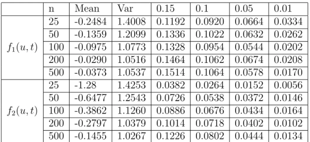
wheref : [0,1]² →Ris some given function andβ : [0,1]→R(i.e. k= 1). The discussion following the proof of Theorem 2.1 states that under the null hypothesisH₀, the statisticT_ndefined in (2.14) converges weakly to a standard normal distribution. We reject the hypothesis H₀ if the inequality (2.14) is satisfied. In order to study the approximation of the nominal level and the power of this asymptotic levelαtest 5000 replications with different functionsf have been performed. The error terms ε(u, t_i) are assumed to be i.i.d. Brownian Motions, i.e. r(t, u, v) =u∧v, which implies that the model is homoscedastic. The results under the null hypothesis are presented in Table 1 for the functions

f₁(u, t) = (−1 + 2u) + 2(1−u)t (5.1)

f₂(u, t) = (1 +u) cos(2πt). (5.2)

It can be seen that the nominal level of the test is well approximated in most cases. For the functionf₁(u, t) = (−1 + 2u) + (2−2u)tthe approximation is very accurate for sample sizes larger than n = 100, for smaller values the level is either overestimated (if the nominal level is smaller than α = 0.1) or underestimated (if the nominal level is larger than α = 0.1). In the case where we use the function f₂(u, t) = (1 +u) cos(2πt) we underestimate the level, with the tendency to get better approximations for larger sample sizes.

For the investigation of the power of the test we consider the functionsf_i defined in (5.1) and (5.2) with two additive alternatives, that is

m(u, t) = fi(u, t) + 1

2exp(t) (5.3)

m(u, t) = f_i(u, t) + sin(2πt) (5.4)

with i= 1,2. The corresponding results are presented in Tables 2 and 3. We observe reasonable rejection probabilities for all sample sizes and both choices of f₁.

Note that for sample sizes n = 25 and n = 50 the approximation of the nominal level is less accurate. In these cases we propose a wild bootstrap procedure to obtain a more accurate test procedure [see Wu (1986)]. For this purpose we denote by ˆβ(u) the (point-wise) ordinary least square estimator of the functionβ(u) and calculate the parametric residuals by

ˆ

ε(u, t_i) = Y_i(u)−β(u)ˆ f₁(u, t_i) (5.5) for i = 1, . . . , n and u ∈ [0,1]. For b = 1, . . . B with B ∈ N let v^b∗_i be independent samples of a random variable V with a Laplacian distribution on the set {−1,1}, and define the bootstrap sample as

Y_i^b∗(u) = ˆβ(u)f1(u, ti) +ε^b∗_i (u); i= 1, . . . , n, (5.6) where

ε^b∗_i (u) =v_i^b∗ ε(u, tˆ _i). (5.7) For each b∈ {1, . . . , B} we calculate the statistic T_n^b∗ =T_n(Y₁^b∗(·), . . . , Y_n^b∗(·)), with T_n as given in (2.14) and denote by

H_n,B^∗ (x) = 1 B

B

X

b=1

I{T_n^b∗ ≤x}

the empirical distribution function of T_n^1∗, . . . , T_n^B∗. We determine the (1− α)-quantile of this distribution and use its quantiles as critical values for the test statistic T_n = T_n(Y₁(·), . . . , Y_n(·)).

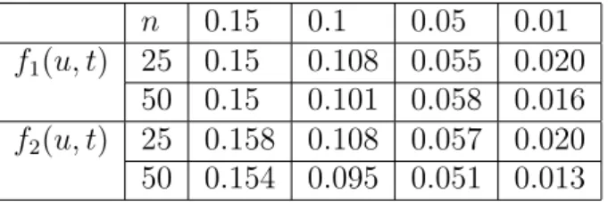
In our simulation study we made 1000 replications of this procedure with B = 200 bootstrap- samples, the corresponding results under the null hypothesis are presented in Table 4 for the sample sizes n = 25 and n = 50, and the regression functions (5.1) and (5.2). Compared to the test based on the normal approximation we observe a substantial improvement with respect to the approximation of the nominal level.

In Table 5 and 6 we show the simulated rejection probabilities of the wild bootstrap test for the alternatives (5.3) and (5.4), respectively. In all cases we obtain similar rejection probabilities as for the test defined in (2.14). Compared to the test based on the asymptotic distribution, a slight loss in power is observed in case of the alternative f_i(u, t) + sin(2πt), while in case of the exponential alternative we observe a negligible improvement for the majority of scenarios.

As a second example we study the finite sample properties of the test for the hypothesis

H₀ :m(u, t) =γ(t)f(u, t), (5.8)

defined in Section 3, where again f : [0,1]² → R is some given function and γ : [0,1] → R (i.e. k = 1). The discussion at the end of Section 3 suggests to reject the hypothesis H₀ if the inequality (3.6) is satisfied. We have investigated the finite sample properties of this test under the assumptions of the previous study forf =f₁ as given in (5.1). The normal approximation did not yield a sufficiently accurate approximations of the level for sample sizes up to n= 500 and for this reason these results are not depicted. As an alternative we propose to use a wild bootstrap approximation similar to the one given in the previous paragraph. More precisely, we calculate residuals analogously to (5.5) by

ˆ

ε(u, t_i) =Y_i(u)−γ(tˆ _i)f₁(u, t_i)

for i = 1, . . . , n and u ∈ [0,1], where ˆγ(ti) denotes the least square estimator for γ(ti). As in equations (5.6) and (5.7) we define

ε^b∗_i (u) = v_i^b∗ ε(u, tˆ _i) and

Y_i^b∗(u) = ˆγ(t_i)f₁(u, t_i) +ε^b∗_i (u) (i= 1, . . . , n)

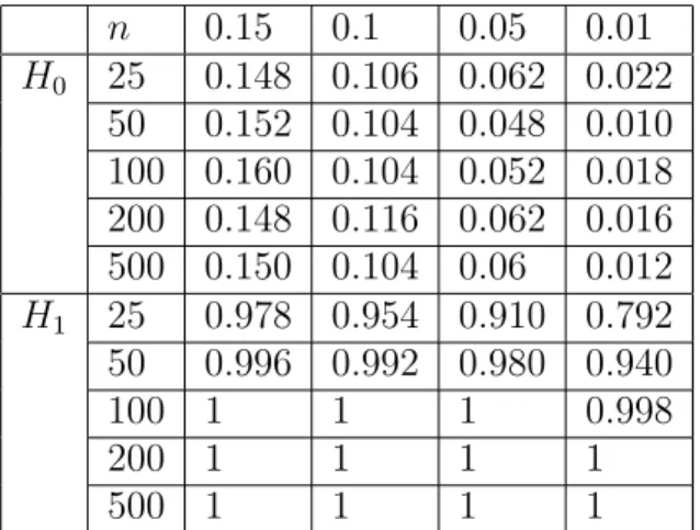
to obtain a wild bootstrap sample. The results of the corresponding bootstrap test are shown in Table 7. We observe that the resampling procedure yields to a test with a very accurate approx- imation of the nominal level and a perfect power behavior under the alternative H₁ : m(u, t) = f₁(u, t) + ¹₂exp(t).

Acknowledgements. The authors would like to thank Martina Stein, who typed parts of this manuscript with considerable technical expertise. This work has been supported in part by the Collaborative Research Center “Statistical modeling of nonlinear dynamic processes” (SFB 823) of the German Research Foundation.